About Canadian historical weather radar
Using Environment and Climate Change Canada's (ECCC) radar data can be quite beneficial when making weather sensitive decisions. To assist users, a comprehensive table of contents, detailing radar information is listed below.
Background
The term RADAR, which has been in use since the 1940s, is an acronym formed from the term Radio Detection and Ranging.
Environment and Climate Change Canada's radar network is concentrated in the most populated parts of Canada, providing coverage to more than 99 per cent of Canadians. The network’s primary purpose is the early detection of developing thunderstorms and high impact weather such as hurricanes, cyclones, tornadoes, floods, severe thunderstorms, and other similar phenomena, as well the tracking of precipitation.
Historical radar images can be accessed through the National Climate Data and Information Archive. Learn how to view the radar images.
How Radar Works
ECCC radars emit brief pulses of radio-frequency energy into the atmosphere, akin to a narrow-beam searchlight, to detect precipitation. When the radar's emitted energy interacts with precipitation particles, a portion is reflected back to the radar. The radar detects and records these returning echoes using highly sensitive receivers. This focused pulsed energy scans the entire sky in a 360-degree sweep around the radar location, changing its elevation angle with each scan. The strength of the reflected energy is connected to the number, size, and type of the precipitation particles.
On public weather platforms such as the weather.gc.ca website or the WeatherCAN app, the maximum range shown for each radar is 240 km. The ECCC's S-Band, denoting a particular set of radio frequencies between 2.7 and 2.9 GHz for its weather radars, can detect targets up to a maximum range of 330 km. However, the Doppler velocity detection range is limited to 240 km. It should be noted that Doppler technology measures the change in frequency (or wavelength) of a wave in relation to an observer moving relative to the source of the wave. In the context of weather, it is crucial for detecting severe weather events, such as tornadoes.
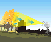
Key Components of Environment and Climate Change Canada’s S-Band Weather Radars

Major components of a weather radar
Graphic illustrating the major components that make up a weather radar including the parabolic antenna, radome ventilation, tower hoist, weather station.
Radar Display Description
There are three views of radar images that can be seen on the Canadian Historical Weather Radar website:
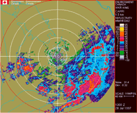
National View
This view provides, at a glance, a complex, low-resolution picture of where precipitation is occurring within the complete ECCC radar network.
The picture is interactive, and can be used to choose the geographical area you are interested in. Clicking on a province will lead you to a Regional View for that area.
From this national picture, you can refine it to view local radar data for a specific geographic region. This can be done by selecting an area near one of the black dots which represent local radar sites.
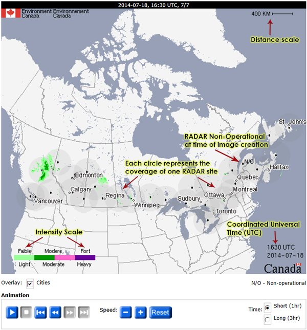
National View of Weather Radar animated graphic for Canada. Click for details.
A map of Canada showing the coverage zones of Environment and Climate Change Canada’s radar stations. The map also explains all the labeling elements that are found on a typical national view radar image.
The radar image can be broken down into three main sections:
Time Stamp
Sample of Time Stamp: 2014-07-18, 16:30 UTC, 7/7
The black bar above the radar map is a timestamp, listing date first, then time in Coordinated Universal Time (UTC), the position of the viewed image, and the total number of images.
Radar image
The sample RADAR image shows where all the radar sites are located in Canada.
Each circle represents the coverage of one radar site. 1 cm represents 400km in distance.
The radar sites are denoted with a black dot. The following major cities are covered in the national view:
- Vancouver, British Columbia
- Edmonton, Alberta
- Calgary, Alberta
- Regina, Saskatchewan
- Winnipeg, Manitoba
- Sudbury, Ontario
- Toronto, Ontario
- Ottawa, Ontario
- Montreal, Quebec
- Quebec City, Quebec
- Halifax, Nova Scotia
- St. John's, Newfoundland
Intensity Scale
The Intensity scale on the bottom left hand of the map shows:
- Light green as the lightest intensity
- Dark green to pink as moderate intensity
- Purple as heavy intensity
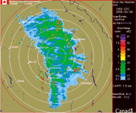
Regional View
This view gives you a higher resolution look at precipitation patterns. The picture is interactive, and can be used to select a more specific area. You can view the actual radar data for a specific geographic region, by selecting an area near one of the black dots representing local radar sites.
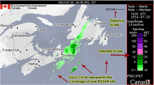
Regional View of weather radar animated graphic for stations located in a region. Click for more details.
A map of Canada showing the coverage zones of Environment Canada’s radar stations. The map also explains all the labeling elements that are found on a typical national view radar image.
The radar image can be broken down into three main sections:
Time stamp
Sample of Time Stamp: 2014-07-25, 16:30 UTC, 7/7
The black bar above the radar map is a timestamp, listing date first, then time in Coordinated Universal Time (UTC), the position of the viewed image, and the total number of images.
RADAR image
The RADAR image shows where all the radar sites are Atlantic Canada. Each circle represents the coverage of one radar site.
1 cm represents 100 km in distance.
The four radar sites in Atlantic Canada cover the following cities:
- Rimouski, Quebec
- Edmunston, New Brunswick
- Frederiction, New Brunswick
- Halifax, Nova Scotia
- Sydney, Nova Scotia
- Charlottetown, Prince Edward Island
- Corner Brook, Newfoundland
- Gander, Newfoundland
- St. John's, Newfoundland
At the time of this image creation, the radar in Val d'Iréne, Quebec was Non-Operational.
Map legend
The map legend to the right of the map shows:
- The regional radar view: Radar - Atlantic
- Universal Coordinated Time: 1630 UTC:
- Date of radar capture: 2014-07-25 :
- Scale: 3.5km/pixel
- Intensity Scale of rain as read by the radar signal.
The intensity scale to the right of the map shows the amount of precipitation that has been detected by the radar. It is measured by decibels relative to Z (dB-Z). The Z is a measure of equivalent reflectivity (Z) of a radar signal reflected off a remote object.
The scale on the left starts from 0.1 mm/hr of rain and goes up 200 mm/hr.
The scale on the right starts from 10 dB-Z and goes up to 61 dB-Z.
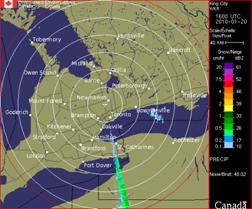
Local View
This is your local view of precipitation detected within the coverage of the local radar site.
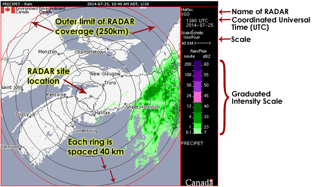
Local View of a weather radar graphic for a station
A sample radar image composite from the station in Halifax, Nova Scotia. The image also explains all the labeling elements that are found on a typical local view radar image.
The radar image can be broken down into three main sections:
Time stamp
The black bar above the sample map shows the following:
- Radar product: PRECIP-Rain
- Local Time: 2014-07-25, 10:40 AM ADT
- Position of the viewed image and the total number of images: 1/10
RADAR image
The sample radar image shows the coverage area for the Halifax, Nova Scotia radar.
Each ring around is spaced 40 km apart. The red circle defines the outer limit of the radar coverage which is 250 km.
The Halifax, Nova Scotia radar encompasses the following areas:
Within an 80 km radius:
- Truro, Nova Scotia
- Halifax, Nova Scotia
- Kentville, Nova Scotia
Within a 120 km radius:
- New Glasgow, Nova Scotia
- Sheet Harbour, Nova Scotia
- Lunenburg, NSNova Scotia
Within a 160 km radius:
- Charlottetown, Prince Edward Island
- Moncton, New Brunswick
Within a 200 km radius:
- Saint John, New Brunswick
- Digby, Nova Scotia
Within a 240 km radius:
- Yarmouth, Nova Scotia
Map legend
The map legend to the right of the map shows:
- Name of the radar and ID code: Halifax XGO
- Time in Coordinated Universal Time (UTC): 1340 UTC
- Date of radar capture: 2014-07-25
- Scale: 1 km/pixel
- Distance Scale. 1 cm represents 40 km
- Graduated Intensity Scale of rain as read by the radar signal. (see below for more details)
- Noise: 85.27 - Technical parameters used by technicians to diagnose the operation of the radar.
The Graduated intensity scale to the right of the map shows the amount of precipitation that has been detected by the radar. It is measured by decibels relative to Z (dB-Z). The Z is a measure of equivalent reflectivity (Z) of a radar signal reflected off a remote object.
The scale on the left starts from 0.1 mm/hr of rain and goes up 200 mm/hr.
The scale on the right starts from 7 dB-Z and goes up to 60 dB-Z.
Radar Interpretation
What am I looking at? (Radar Echoes)
When you look at a radar image, you are looking at a picture of precipitation distribution (called “echoes”) and its intensity.
Radar echoes are represented by a series of coloured pixels, as illustrated on the scale to the right of the radar image. The intensity scale on the right represents what is called “reflectivity in dBZ” (unit of reflectivity), and the scale on the left is the corresponding rate of fall which is an interpretation of how light or heavy the precipitation is. In the winter season, this reflectivity is linked to the snowfall rate in centimetres per hour (cm/hr), and in the summer months, the reflectivity is linked to the rainfall rate in millimeters per hour (mm/hr).
How to understand precipitation information? (Reflectivity)
The higher the reflectivity value on a radar image, the heavier the precipitation rate that is being detected.
For example, the dark purple colour represents the heaviest precipitation of snow (meaning it has a snow rate of fall of 20 cm/hr). The aqua colour is the lightest precipitation (meaning it has a snow rate of fall of 0.1cm/hr).
Reflectivity not only depends on the precipitation intensity, but also the type of precipitation. Snow generally reflects less radar energy than rain. Consequently, moderate to heavy snow can appear light in intensity. Meanwhile, ice pellets and hail are highly reflective so light ice pellets or hail can appear as heavy precipitation.
In some cases, the radar does not distinguish between real echoes (precipitation) and non-meteorological echoes (trees, hills, tall buildings). It is also important to understand some common interpretation errors, if you are hoping to accurately interpret the radar images.
What is a DPQPE product?
DPQPE stands for, “Dual-Pol Quantitative Precipitation Estimation. It is a two-dimensional representation of the precipitation rate estimated by the lowest sweep of the radar (elevation angle of 0.4 degrees for the majority of S-Band radars). Thus, the precipitation rate is estimated as close to the earth's surface as possible. The DPQPE product is based, among other things, on a series of polarimetric processing steps (quality control) to eliminate non-meteorological artifacts from the raw data (volumetric scans). It renders in mm/h for rain and cm/h for snow. This product is calculated with a maximum coverage range of 240 km.
For more information about the Canadian Weather Radar.
What is a PRECIP-ET Product?
Since the old C-Band radars have been replaced by the new S-Band radars, PRECIP has been replaced by "PRECIP-ET" (PRECIPitation-ExTended). The last C-Band radar was replaced on August 21, 2023 and the PRECIP product is now available in our archives only.
The type of image you are viewing is indicated at the bottom right-hand legend.
PRECIP-ET images
The PRECIP-ET (PRECIPET on images) is an extension of the PRECIP product (hence the use of ET in the product name). Compared to the previous PRECIP product, the PRECIP-ET performs a suite of additional quality control tests and tracks issues better. For example, Doppler filters might be rejecting moderate ground echoes in a particular area and thus weak meteorological echoes would not be detectible. In this case, PRECIP-ET would flag the missing data area, whereas PRECIP would simply treat the area as no echoes. This additional quality treatment is why we have migrated to PRECIP-ET in 2013, to get an improved service.
The PRECIP-ET image is designed to show the precipitation close to the ground, by using Doppler technology processing for echoes within 128 km from the radar site for the C-Band radars. Doppler technology allows for better resolution of the precipitation echoes and also provides the ability to detect the movement of precipitation in relation to the radar (i.e. are the raindrops or snowflakes moving towards or away from the radar and at what speed). Beyond this 128 km limit, the echoes are displayed using the more conventional CAPPI processing which is explained below.
Differences between PRECIP-ET and PRECIP:
- Non-meteorological echoes : Weather radars can receive non-meteorological echoes from ground objects such as buildings and towers; the PRECIP-ET product uses Doppler processing to edit out most of these false echoes. Doppler processing can detect these non-meteorological echoes because they are not moving in relation to the radar as the realistic precipitations as raindrops and snowflakes would. So, with the clutter caused by ground objects filtered out, the PRECIP-ET product provides a cleaner image close to the radar. In addition to the direct Doppler corrections, PRECIP-ET looks at patterns of echoes and attempts to remove echo patterns that do not appear meteorological. For example, if the radar implies very strong precipitation near the surface, then there should be a big storm above it. This process is more ambiguous than simple Doppler as some false targets look like precipitation and vice-versa, so the removal of many non-meteorological targets may lead to occasional removal of valid precipitation.
- Blocked radar beams: Trees and hills around radars can block portions or the entire radar beams, resulting in a decreased ability to detect precipitation close to the ground near the radar. This problem can be particularly obvious during winter months when a lot of precipitation forms and falls close to the ground. Therefore with some or most of the radar beam being blocked in the very low levels during the winter, the radar may not do the best job at detecting light precipitation near the radar, and why no echoes does not necessarily mean no snow in reality close to the radar.
- Discontinuity: Doppler processing is not as efficient, in general, at detecting weak precipitation as conventional radar processing is. Since the PRECIP-ET product is a combination of Doppler processing (first 110 km from radar) and conventional processing (beyond 110 km from the radar), there can sometimes appear to be a discontinuity in the precipitation as one goes beyond 110 km from the radar.
What is the difference between PRECIP-ET-Rain and PRECIP-ET-Snow images?
In general, rain is more easily detected by radar than snow. In order to better represent precipitation during the warm season, a certain relationship is used to relate the reflectivity to a rainfall rate (in mm/h - PRECIPET-Rain). During the cold season, a different relationship is used to relate the reflectivity to a snowfall rate (in cm/h - PRECIP-ET-Snow). However, a reflectivity presented in mm/h isn’t necessarily rain, while a reflectivity presented in cm/h isn’t necessarily snow. The precipitation in most of the more densely populated areas of the country can still show a high degree of variability in the fall, winter and spring allowing for rain, freezing rain, ice pellets and snow to occur alone or in some combination. Therefore, it is always important to relate the precipitation you are seeing on radar with what the current weather conditions are and what the forecast is in the coming hours to get the best sense of what may fall out of the sky in your area.
What is a CAPPI Radar Product?
Due to the curvature of the Earth, the height of a radar beam, in relation to the ground, increases as it travels further from the radar. When the radar is pointed down near the ground (a low elevation angle), the beam starts off near the ground but then its height above the ground slowly increases. By the time that same beam is 200 km from the radar, it is at a height of around 4 km above the ground. In order to get a better sense of what is happening at one approximate height above the ground (i.e. 1.5 km), a whole series of radar beams with different elevation angles (low, medium, high) are used to create one radar product. This type of radar product is called a CAPPI (Constant Altitude Plan Position Indicator). Since the CAPPI products do not use Doppler processing to filter out clutter like tall trees, hills and buildings, it can sometimes be contaminated by non meteorological echoes.
Common Interpretation Errors
Sometimes what you see is not necessarily what you get. Just because something looks colourful on the radar screen does not mean there is rain or snow. Similarly, just because the echoes on the screen appear weak or do not appear at all, this does not mean there is not significant precipitation falling somewhere.
Here are some of the more common radar interpretation mistakes:
Blocking Beam
Hills and mountains can block a radar beam and leave noticeable gaps in the pattern.
This situation is very common in the Rockies and Newfoundland, due to the hilly terrain.
As well, with the new S-Band radars there are cases where there is a wedge shaped gap. In some cases these are a blanked sector in the direction of a permanent or temporary obstacle. For example, there is a permanent blanked sector to the west of the Spirit River radar (254° - 266°) in the direction of a nearby tower. Our radar does not transmit in that direction. These blanked sectors may be only temporary for example if there is work being done on a nearby tower.
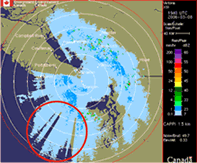
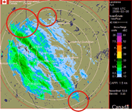
Beam Attenuation
Storms closest to a radar site reflect or absorb most of the available radar energy. Only a reduced amount of this energy is available to detect more distant storms. This situation is much improved with the S-Band radars as they have significantly reduced attenuation issues.
Storms in the below example’s circled area were quite intense, but were not being detected appropriately by the radar. Strong storms occurring closer to the radar kept a significant portion of the radar energy from penetrating beyond these storms.

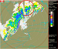
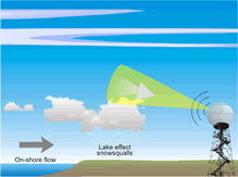
Overshooting Beam
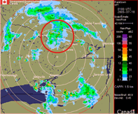
Intense precipitation, such as lake effect snow squalls, can be associated with clouds close to the ground. In such cases, the radar beam may overshoot most of the area of precipitation and therefore indicate only weak echoes, when in fact significant precipitation is occurring.
The example image shows lines of precipitation on the Prairies. Although it was raining inside the radar coverage area, the radar overshoots at long range and the bands are not seen.
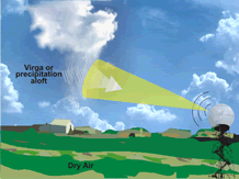
Virga
Precipitation that is occurring in the air but not reaching the ground, is called virga. It happens when there are dry conditions at low levels and the dry air absorbs all the moisture before it reaches the ground. No precipitation was hitting the ground in the example attached.
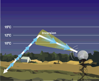
Anomalous Propagation (AP)
In the low levels of the atmosphere when a layer of warm air lies over a layer of much cooler air (a temperature inversion), the radar beam can't pass between the layers, and gets bent to the ground. A false strong signal is reflected back to the radar site.
This phenomenon is most common during the early morning hours when it is clear. The false echoes generally dissipate by midday.
In the example image below, there was no precipitation occurring.
Ground Clutter
Ground clutter is echoes that happen when a portion of the radar beam comes into contact with tall buildings, trees or hills. It is good to learn the common ground clutter "signature" in your area, so you can distinguish it from real precipitation.
Radars near large bodies of water may also receive echoes from moving waves. Since waves depend on wind speed and direction, sea clutter is more variable than standard ground clutter and is therefore more difficult for existing processing to filter out.

Electromagnetic Interference
The historical Environment and Climate Change Canada radar network is heterogeneous. A frequency range of 2.7 - 2.9 GHz is used for S-band radars. ECCC operates each weather radar at a specific frequency band specified by Innovation, Science and Economic Development Canada (ISEDC). Sometimes external sources, either at the same frequency or combined to be the same frequency, can be detected in our radar systems. Once these interference issues are detected, ISEDC is notified to find the source, which can be challenging. In moderate to severe weather, weather signals generally overshadow these interference signals, and using the information from the dual polarization technology that ECCC is deploying can help resolve some of these problems in lighter precipitation.
Typical interference from a wireless device appears as a persistent spike on the radar going out from the radar in one direction (i.e. along a radial). A typical spike is shown in the image below. Sometimes a “sun spike” can be briefly seen at sunrise or sunset when the radar has a clear view of the sun low on the horizon. This is caused by the solar radiation being picked up by the sensitive radar receiver.