Health impacts of traffic-related air pollution in Canada

March 2022

Table of contents

• List of tables
• List of figures
• List of abbreviations
• Executive summary
• 1. Introduction
• 2. Methodology
  • 2.1 Emissions inventory
  • 2.2 Air quality modelling
    • 2.2.1 Chemical transport model
    • 2.2.2 Simulation approach
    • 2.2.3 Model output
  • 2.3 Health impact assessment
    • 2.3.1 Calculating population health impacts due to air pollution
    • 2.3.2 Calculating the economic value of health outcomes due to air pollution
• 3. Results
  • 3.1 Emissions associated with on-road transportation
  • 3.2 Modelled contributions from TRAP to ambient air pollution
    • 3.2.1 Fine particulate matter
    • 3.2.2 Nitrogen dioxide
    • 3.2.3 Ozone – summer
    • 3.2.4 Ozone – annual
    • 3.2.5 Sulphur dioxide
  • 3.3 Modelled air pollution health impacts
• 4. Discussion
  • 4.1 Emissions inventory and modelled air quality
  • 4.2 Estimates of population health burden
    • 4.2.1 Comparison with previous assessments of air pollution health impacts linked to on-road diesel and gasoline vehicle emissions in Canada
  • 4.3 Methodological considerations
    • 4.3.1 Emissions inventory
    • 4.3.2 Air quality modelling
      • 4.3.2.1 Geographic scale and grid resolution
      • 4.3.2.2 Unaccounted-for chemical mechanisms and secondary pollutants
      • 4.3.2.3 Averaging times
      • 4.3.2.4 Modelling approach
      • 4.3.2.5 Model performance analysis
    • 4.3.3 Estimates of population health burden
      • 4.3.3.1 Concentration–response functions
      • 4.3.3.2 Geographic and temporal resolution of health burden estimates
• 5. Conclusion
• 6. References
• 7. Appendices
  • Appendix A – GEM-MACH and AQBAT methodology – Additional information
    • A.1 Emissions modelling
      • Biogenic emissions
      • Anthropogenic emissions
    • A.2 GEM-MACH modelling
    • A.3 AQBAT – health endpoints and valuation
    • A.4 References
  • Appendix B – Air emissions – Additional information, tables and figures
  • Appendix C – Ambient air concentrations – Additional information, tables and figures
  • Appendix D – Base case model performance analysis

List of tables

• Table 1. Air pollutant emissions in Canada, in tonnes, for the year 2015 – Source categories and classes, and transportation sub-classes
• Table 2. Percentage of provincial and territorial emissions from on-road transport in 2015
• Table 3. Contributions from Canadian on-road vehicle emissions to ambient PM2.5 concentrations in 2015 – Provincial, territorial, and national estimates – Population-weighted annual average
• Table 4. Contributions from Canadian on-road vehicle emissions to ambient PM2.5 concentrations in 2015 – CDs with the highest net contributions – Area-weighted annual average
• Table 5. Contributions from Canadian on-road vehicle emissions to ambient NO2 concentrations in 2015 – Provincial, territorial, and national estimates – Population-weighted annual average
• Table 6. Contributions from Canadian on-road vehicle emissions to ambient NO2 concentrations in 2015 – CDs with the highest net contributions – Area-weighted annual average
• Table 7. Contribution from Canadian on-road vehicle emissions to ambient summer O3 concentrations in 2015 – Provincial, territorial, and national estimates – Population-weighted summer average of daily maximum values
• Table 8. Contribution from Canadian on-road vehicle emissions to summer O3 concentrations in 2015 – CDs with the highest net contributions – Area-weighted summer average of daily maximum values
• Table 9. Contribution from Canadian on-road vehicle emissions to ambient annual O3 concentrations in 2015 – Provincial, territorial, and national estimates – Population-weighted annual average of daily maximum values
• Table 10. Contribution from Canadian on-road vehicle emissions to ambient annual O3 concentrations in 2015 – CDs with the highest net contributions – Area-weighted annual average of daily maximum values
• Table 11. Contribution from Canadian on-road vehicle emissions to ambient annual O3 concentrations in 2015 – CDs with negative estimates – Area-weighted annual average of daily maximum values
• Table 12. Contributions from Canadian on-road vehicle emissions to ambient SO2 concentrations in 2015 – Provincial, territorial, and national estimates – Population-weighted annual average
• Table 13. National estimates of premature deaths and non-fatal health outcomes associated with exposure to TRAP from Canadian sources in 2015, by health endpoint – Counts and valuation
• Table 14. Premature deaths associated with exposure to TRAP in 2015, by pollutant – Provincial and national estimates – Counts and rates per 100,000 population
• Table 15. Premature deaths associated with exposure to TRAP from Canadian sources in 2015, by pollutant – Census divisions with the highest estimates – Counts and rates per 100,000 population
• Table 16. Contributions from on-road vehicle emissions to ambient concentrations of NO2, O3 and PM2.5 in 2015 – Provincial and territorial population-weighted averages and maximum area-weighted CD estimates
• Table 17. Contributions from Canadian on-road gasoline vehicle emissions, on-road diesel vehicle emissions, and TRAP to ambient PM2.5 concentrations in 2015 – Provincial and national estimates – Population-weighted annual average
• Table 18. Contributions from Canadian on-road gasoline vehicle emissions, on-road diesel vehicle emissions, and TRAP to ambient NO2 concentrations in 2015 – Provincial and national estimates – Population-weighted annual average
• Table 19. Contributions from on-road gasoline vehicle emissions, on-road diesel vehicle emissions and TRAP to summer average ambient 1-hour maximum O3 concentrations in 2015 – Provincial and national estimates – Population-weighted annual average
• Table 20. Premature death associated with Canadian on-road gasoline vehicle emissions, on-road diesel vehicle emissions and all on-road vehicle emissions using various CRFs for PM2.5 chronic exposure mortality – National estimates for calendar year 2015
• Table 21. Annual performance evaluation statistics comparing the 2015 base case estimates in GEM-MACH and 2017 observations

List of figures

• Figure 1. On-road heavy-duty (HDV) and light-duty (LDV) vehicle emissions in Canada, based on the 2015 inventory
• Figure 2. Heavy-duty vehicle emissions in the 2015 Canadian emissions inventory
• Figure 3. Light-duty vehicle emissions in the 2015 Canadian emissions inventory
• Figure 4. Net contribution (µg/m3) from Canadian on-road vehicle emissions to annual average PM2.5 concentrations in 2015
• Figure 5. Net contribution (ppbv) from Canadian on-road vehicle emissions to annual average NO2 concentrations in 2015
• Figure 6. Net contribution (ppbv) from Canadian on-road vehicle emissions to summer average daily maximum O3 concentrations in 2015
• Figure 7. Net contribution (ppbv) from Canadian on-road vehicle emissions to annual average daily maximum O3 concentrations in 2015

List of abbreviations

ADOM

Acid Deposition Oxidant Model

APEI

Air Pollutant Emissions Inventory

AQBAT

Air Quality Benefits Assessment Tool

AURAMS

A Unified Regional Air Quality Modelling System

CAD

Canadian dollar

CD

Census division

CM

Crustal material

CO

Carbon monoxide

COPD

Chronic obstructive pulmonary disease

CRF

Concentration response function

CTM

Chemical transport model

EC

Elemental carbon

ECCC

Environment and Climate Change Canada

GEM

Global Environmental Multiscale (weather forecast model)

GEM-MACH

Global Environmental Multiscale – Modelling Air Quality & Chemistry

GIS

Geographic information system

GTHA

Greater Toronto and Hamilton Area

HDV

Heavy-duty vehicle

HDV8

Class 8 heavy-duty vehicle

HEI

Health Effects Institute

HPC

High Performance Computing

IHD

Ischemic heart disease

IHME

Institute for Health Metrics and Evaluation

LDDT

Light-duty diesel truck

LDT

Light-duty truck

LDV

Light-duty vehicle

µg/m³

Micrograms per cubic metre

MBE

Mean bias error

MOVES

Motor Vehicle Emission Simulator

NH₃

Ammonia

NO₂

Nitrogen dioxide

NO₃

Ammonium

O₃

Ozone

PM_2.5

Fine particulate matter

POA

Primary organic aerosol

ppb

Part per billion by volume

ppm

Part per million

RMSE

Root mean square error

SMOKE

Sparse Matrix Operator Kernel Emissions

SO₂

Sulphur dioxide

SOA

Secondary organic aerosol

TRAP

Traffic-related air pollution

TWBL

Tire wear and brake lining

US EPA

United States Environmental Protection Agency

VAQUM

Verification of Air Quality Models

VOC

Volatile organic compound

WHO

World Health Organization

WTP

Willingness to pay

Executive summary

A large body of scientific evidence has accumulated over the past 25 years attributing a wide range of adverse health effects to ambient (outdoor) air pollution exposure. These effects range in severity from respiratory symptoms to the development of disease and premature death. For example, exposure to airborne particles, a component of smog, increases the risk of premature mortality from heart disease, stroke and lung cancer.

On-road vehicles contribute to air pollution through fuel combustion and evaporative emissions as well as emissions from tire and brake wear. Canadians are regularly exposed to traffic-related air pollution (TRAP), most notably in high-traffic areas such as near highways and urban centres. TRAP consists of a complex and variable mixture of particulate and gaseous pollutants that contribute to smog, including fine particulate matter (PM_2.5) and ozone (O₃).

The objective of this report is to present modelled estimates of population health impacts and socio-economic costs associated with exposure to TRAP in Canada for the year 2015, specifically the contribution from Canadian on-road vehicle emissions to PM_2.5, NO₂ and O₃ ambient concentrations in Canada. The year 2015 was selected for modelling based on data availability and quality considerations. Results at the national, provincial and territorial, and census division level are presented and discussed. The report is intended to inform Canadian authorities on the air quality and health impacts associated with on-road vehicle activity.

This report estimates that TRAP was associated with over 1,200 premature deaths in Canada in 2015. Of these, it was estimated that exposure to PM_2.5, NO₂ and O₃ contributed to 800, 340 and 85 premature deaths, respectively. Non-fatal health outcomes included 2.7 million acute respiratory symptom days, 1.1 million restricted activity days and 210,000 asthma symptom days per year. The total annual monetary value of the health burden was estimated at $9.5 billion (CAD 2015), with $9 billion being associated with premature deaths. Analysis also found that light-duty vehicles (e.g. passenger vehicles) contributed to approximately 37% of premature deaths, while heavy-duty vehicles (e.g. commercial trucks and buses) contributed to approximately 63% of premature deaths. In terms of the geographic distribution of the air pollution burden, the results indicated greater adverse health impacts in more populous provinces and census divisions (CDs): 500 premature deaths were estimated in Ontario, 410 in Quebec, 170 in British Columbia and 82 in Alberta. At the CD level, 170 premature deaths were estimated in Toronto, 150 in Montreal, and 110 in Vancouver. The results from this analysis are available for all CDs and can be obtained upon request from Health Canada.

The air quality modelling for this analysis was conducted at a grid resolution of 10 km, which is a reasonably high resolution for a national assessment. However, 10-km grid cells are too coarse to capture the local variability and magnitude in exposures to TRAP, such as those experienced by populations near high-traffic roadways. This limitation likely leads to an underestimation of population exposure to TRAP and health impacts, so that the values herein possibly represent a lower range estimate.

This analysis contributes to our understanding of the health burden of exposure to TRAP in Canada. It also complements recent and ongoing activities on TRAP at Health Canada, including health risk assessments and an evaluation of exposure to TRAP in Canada. Together, these analyses are intended to provide a comprehensive national evaluation of TRAP in Canada.

1. Introduction

A large body of scientific evidence has accumulated over the past 25 years attributing a wide range of adverse health effects to ambient (outdoor) air pollution exposure. These effects range in severity from respiratory symptoms to the development of disease and premature death. For example, exposure to airborne particles, a component of smog, increases the risk of premature mortality from heart disease, stroke and lung cancer. In Canada and internationally, health impact assessments identify air pollution as one of the top risk factors for premature mortality and several non-fatal outcomes (WHO 2016). Exposure to air pollution is currently considered the fifth leading mortality health risk in the world and, in 2017, was responsible for 4.9 million premature mortalities, or 8.7% of all deaths globally (IHME and HEI 2019). Burnett et al. (2018) attributed 8.9 million deaths in 2015 to exposure to ambient fine particulate matter (PM_2.5) alone.

Health Canada estimated that 15,300 premature deaths in Canada were associated with ambient air pollution exposure in 2016 (Health Canada 2021). For their analysis, Health Canada defined air pollution as the above-background increment of ambient PM_2.5, nitrogen dioxide (NO₂) and ozone (O₃) concentrations that can be attributed to anthropogenic North American sources of emissions (e.g., fuel combustion, industry, etc.), as well as emissions from natural events such as wildfires. Non-fatal outcomes were also estimated, including 2.7 million asthma symptom days per year and 35 million acute respiratory symptom days, with the total economic cost of all health impacts attributable to air pollution in 2016 Canadian dollars (CAD 2016) being $120 billion (Health Canada 2021).

The contribution from on-road vehicles to ambient air pollution is referred to as traffic-related air pollution (TRAP). Most Canadians experience exposure to TRAP on a daily basis, particularly in high-traffic areas such as near highways and in urban centres (Brauer et al. 2012, 2013; Matz et al. 2018). TRAP consists of a mixture of particulate and gaseous pollutants associated with combustion (i.e. vehicle exhaust) and non-combustion (e.g. fuel evaporation, abrasion wear) processes. TRAP can influence ambient concentrations of several air pollutants, including PM_2.5 and O₃ that are responsible for smog. Owing to its complex and variable composition, the TRAP mixture cannot be measured directly. It is generally estimated using a limited number of measurable surrogates, such as NO₂ or ultrafine particulate matter, which involves some uncertainties.

The objective of this report is to present estimates of population health impacts and costs associated with exposure to TRAP in Canada. The results are intended to inform Canadians and provincial, territorial and regional stakeholders of the air quality and health impacts associated with on-road vehicle activity. This analysis focuses on the contribution of Canadian on-road vehicle emissions to ambient concentrations of PM_2.5, NO₂, O₃ and sulphur dioxide (SO₂) for the year 2015, and the associated health impacts for PM_2.5, NO₂ and O₃, including premature death and morbidity, in Canada. Traffic is defined as on-road transportation and corresponds to the category on-road vehicles in Canada's Air Pollutant Emissions Inventory (APEI). These include light-duty vehicles and trucks, motorcycles, buses, and medium-duty and heavy-duty vehicles. Vehicles used for off-road applications, such as agricultural and mining equipment, are excluded from the on-road category. Health Canada collaborated with Environment and Climate Change Canada (ECCC) to estimate the ambient air pollution attributable to TRAP across Canada, interpreted herein as the exposure to TRAP. To estimate exposure, the Global Environmental Multiscale – Modelling Air Quality and Chemistry (GEM-MACH) model was used. The air quality modelling for this analysis was conducted at a grid resolution of 10 km. The air quality modelling results were then averaged over Canadian census divisions (CDs), which vary in size. The modelling approach and regional resolution were selected for this national assessment. It does not capture the local variability and magnitude in exposures to TRAP, such as those experienced by populations near high-traffic roadways.

Health Canada used the output from the air quality modelling to estimate TRAP population health impacts as well as the monetary value of the related health burden across Canada using the Air Quality Benefits Assessment Tool (AQBAT). This modelling-based analysis considered exposure to ambient levels of PM_2.5, O₃ and NO₂. Air quality and health impacts associated with other toxic air pollutants in TRAP, including SO₂, carbon monoxide (CO), organic compounds (e.g. volatile organic compounds such as formaldehyde and benzene, polycyclic aromatic compounds), ultrafine particulate matter (UFP) or specific PM_2.5-associated compounds (e.g., metals, polycyclic aromatic compounds), were not included. The health impact assessment provides results at the national, provincial, territorial and census division levels. As such, the health impact estimates reflect average regional air pollution exposures rather than local or high pollution microenvironment exposures, such as in near-road environments.

The current analysis complements and updates previous health impact analyses for diesel- and gasoline-related air pollution published by Health Canada (2016a, 2017). It uses updated data and modelling tools to investigate the health impacts of all on-road sources and fuel types. The analysis also complements risk assessment activities at Health Canada conducted to inform and support programs and policies designed to mitigate exposure to, and health impacts of, air pollution in Canada. This includes a report evaluating the role of exposure to TRAP in asthma, allergy, and lung function using a weight of evidence approach (Health Canada 2020). Health Canada is also assessing exposure to TRAP in Canada based on a literature review and an analysis of population proximity to roadways. Together, the Health Canada assessments of health risks, population health burden, exposures associated with TRAP in Canada are intended to provide a comprehensive national evaluation.

This report summarizes the methodological approach and the results for each step of the health impact modelling framework, including the air pollutant emissions inventory, the air quality (i.e., ambient air concentrations) modelling simulations, the health impact assessment, and the estimate of socio-economic costs (valuation). Results at the national, provincial and territorial, and census division level are presented and discussed.

2. Methodology

The air pollution and health burden estimates are based on a modelling framework designed for the analysis of source sectors, including on-road vehicles. The modelling framework for this analysis utilizes three main steps and tools that are discussed in sections 2.1 to 2.3:

1. Air pollutant emissions inventory;
2. Chemical transport modelling of air pollution scenarios; and
3. Health impact assessment and valuation.

The general approach was to develop an emissions inventory for the year 2015 (step 1), which included detailed data for traffic and other source sectors of air pollution. In step 2, ambient air pollutant concentrations were estimated using a chemical transport model (CTM). Concentrations attributable to TRAP were determined by comparing the air quality estimates from the CTM for a reference emissions scenario and for a scenario involving complete removal of on-road vehicle emissions. The difference between the two scenarios corresponded to the estimate of the contribution of TRAP to ambient air pollution concentrations. In step 3, TRAP concentrations were input into the Air Quality Benefits Assessment Tool (AQBAT) to estimate the population health burden attributable to TRAP in Canada, including mortality and morbidity outcomes, as well as socio-economic costs. Additional methodological details of the modelling framework are presented in Appendix A.

2.1 Emissions inventory

ECCC developed a detailed emissions inventory for the year 2015, based on the 2017 Air Pollutant Emissions Inventory, to be used as input to the chemical transport model.^{Footnote 1} It was the most recent and accurate version available when the modelling analysis was initiated. The emissions inventory used for the United States was the 2017 projection emissions inventory based on the United States Environmental Protection Agency (US EPA) 2011 National Emissions Inventory (NEI).^{Footnote 2} The 2008 inventory used for Mexico (Inventario Nacional de Emisiones, INEM)^{Footnote 3} was also from the US EPA 2011 NEI. The emission estimates were chemically speciated, spatially distributed, and temporally resolved. ECCC used different approaches and data to develop the emissions inventory, including industrial pollutant release data, fuel use data, source-specific activity data and emission factors (ECCC 2015, 2016). Primary emissions were estimated for both anthropogenic and biogenic source categories (except emissions from wildfires). Additional methodological details of emissions modelling are presented in Appendix A.

On-road vehicle emissions were estimated using the Motor Vehicle Emission Simulator (MOVES) version 2014b, developed by the US EPA. The model has been modified to reflect Canadian conditions, such as vehicle population and age distribution, as well as vehicle emission standards. MOVES provides emission rates for a series of pollutants, including CO, ammonia (NH₃), nitrogen oxides (NOx), PM, SO2 and volatile organic compounds (VOCs), which are then combined with vehicle activity data. Traffic source emissions modelled by MOVES and considered in this analysis included exhaust, evaporative and tire wear and brake lining (TWBL) emissions from gasoline and diesel on-road vehicles, as well as on-road vehicles powered by other fuels (e.g., compressed natural gas). Evaporative emissions from stationary sites, such as those from refuelling stations or fuel storage facilities, were not included as a component of TRAP; they are associated with air pollutant emissions from commercial, institutional, or industrial sources. Dust emissions from paved and unpaved roads were also excluded as a component of TRAP; they are associated with open sources^{Footnote 4} in the APEI and are not allocated to specific segments of the vehicle fleet. On-road transportation emissions were compiled as monthly values for different vehicle types and aggregated at the provincial level, except for British Columbia and Ontario. Sub-provincial vehicle information was available for these two provinces (e.g., inspection and maintenance programs), allowing the creation of sub-regions (two for British Columbia and four for Ontario). Five different road classes were also used to improve the spatial allocation of on-road vehicle emissions: rural restricted and unrestricted access, urban restricted and unrestricted access, and off-network. For on-road transportation emissions specifically, Canadian engine emission standards and fuel regulations effective in 2015 were considered.^{Footnote 5}

The 2015 inventory database was further processed by ECCC to generate a dataset that can be used in the Sparse Matrix Operator Kernel Emissions (SMOKE) model (Sassi et al. 2016). Spatial surrogates from SMOKE version 3.7 (in ASCII format), generated from geographic information system (GIS) shapefiles, were used to allocate emissions to a national grid surface. Ancillary and updated shapefiles were also included to distribute emissions across Canada. The spatially allocated emissions became input to the chemical transport model.

2.2 Air quality modelling

2.2.1 Chemical transport model

The chemical transport model used for this assessment was ECCC's Global Environmental Multiscale – Modelling Air Quality and Chemistry (GEM-MACH) model, version 2.3.1. GEM-MACH, a source-oriented Eulerian model, is a prognostic tool that integrates meteorological data and specific algorithms to simulate the diffusion, transport and chemical transformation of gases and particles in the atmosphere (Makar et al. 2018; Moran et al. 2010; Whaley et al. 2018, 2020). GEM-MACH is used by ECCC to simulate hourly concentrations of air pollutants including O₃, PM_2.5, NO₂, and SO₂ over a North American domain, for operational air quality forecasting and in support of air quality regulations and management decisions for Canada.

The general air quality modelling approach included simulations conducted over a continental domain with a horizontal grid spacing of 10 km by 10 km, and 80 hybrid vertical levels extending from the surface (1.5 m) to 0.1 hectopascal (approximately 30 km). GEM-MACH simulations were done for a complete year, computing 24 hours of forecast for each day. The model's time step is 300 seconds, such that meteorological and atmospheric conditions are computed every five minutes. Hourly output values (i.e., pollutant concentrations) are simulated. Simulations were conducted using 2017 meteorology that corresponds to forecasts produced operationally on a daily basis by ECCC in 2017. It includes data assimilation of observations.

The GEM-MACH model was executed on ECCC's High Performance Computing (HPC) system. The simulation was divided into four three-month segments, each with a 21-day spin-up period. The segments correspond to January–March, April–June, July–September and October–December. All segments are computed in parallel to decrease the execution time. A task sequencer is used to manage and submit on the HPC the different steps required to perform an uninterrupted simulation.

The post-processing of GEM-MACH results consists of computing different statistics by using an automated suite of tools, such as Kornshell and Tcl scripts, as well as C/C++ and Fortran programs. The statistics include, for example, averages, rolling averages, maximum values and differences between scenarios, for different periods (monthly, annual and seasonal). Statistics are computed for the model grid and can be interpolated on different geographical areas, such as census divisions (CDs) as used in AQBAT. The final products are available in formats such as ASCII, binary, GIS, and graphical format, depending on the research objectives.

From the gridded modelled results, ambient air pollution estimates were generated at the CD level for NO₂, O₃, PM_2.5 and SO₂ for linkage with AQBAT. The results represent regional air pollution conditions and do not reflect local effects and microenvironments that are unresolved by the horizontal grid size, such as roadways and street canyons, where air pollution levels may be higher. Appendix A presents additional methodological details of the GEM-MACH model. Methodological considerations are discussed in section 4.3.

2.2.2 Simulation approach

In order to isolate the contribution of TRAP to ambient pollutant concentrations in Canada, a brute force approach was used wherein two air quality scenarios were modelled with GEM-MACH: (1) a reference scenario with the full Canadian 2015 emissions inventory and (2) a TRAP scenario with on-road vehicle emissions removed from the inventory. The TRAP scenario required zeroing-out all Canadian air pollutant emissions in Canada from motorcycles, light-duty vehicles and heavy-duty vehicles for the calendar year 2015. The differences in air quality between the full emissions inventory scenario and the scenario with Canadian on-road vehicle emissions removed are assumed to represent the contribution to ambient pollutant levels from on-road vehicles in Canada. This increment is also used to estimate the population exposure to TRAP.

2.2.3 Model output

Ground-level concentrations were estimated for each model grid cell and Canadian CD for the following pollutants and concentration metrics:

• Annual average based on:
  • hourly data for NO₂, PM₅, and SO₂
  • daily maximum of hourly data for O₃
• Summer (i.e., May–September) average based on daily maximum of hourly data for O₃

The units for NO₂, O₃ and SO₂ are in parts per billion by volume (ppbv), while PM_2.5 values are in micrograms per cubic metre (µg/m³). For the current analysis, estimates of ground-level concentrations were not available for all air pollutants in the emissions inventory, including CO and PM₁₀.

Concentration estimates are reported for each province and territory as well as for some individual CDs (section 3.2). For the current analysis, the CDs were based on the Standard Geographical Classification 2011, which divides Canada into 293 CDs.^{Footnote 6} The CD air pollutant concentrations are area-weighted estimates from the original GEM-MACH grid. Area-weighted concentrations for each CD were determined by summing the product of a grid cell concentration and the area of that grid cell occupied by the CD, for all grid cells intersecting with the CD, and then dividing the sum by the area of the CD. For example, if three grid cells intersect with a CD, the following formula would apply to determine its concentration (C_d):

C_d = (A_d1 × C_g1 + A_d2 × C_g2 + A_d3 × C_g3) ÷ A_d

where A_dx is the area of overlap between the model grid cells and the CD, C_gx is the concentration of the grid cell gx, and A_d is the area of the CD.

The reported national, provincial and territorial concentrations correspond to population-weighted estimates. The population-weighting method estimates the average exposure concentration for an individual within a geographic unit. When averaged across larger geographic units, CDs with high populations have more influence or weight than CDs with low populations. Compared to an area-weighted measure, population-weighting provides a better representation of the average pollutant concentration to which Canadians are exposed. This is especially important in Canada as populations are generally limited to urban areas in the southern portion of the country, compared with the vast rural and low population northern areas.

Population-weighted concentrations for all provinces and territories were determined by summing the product of a CD concentration and the population of that CD, for all CDs in a province, and then dividing the sum by the provincial population. For example, if a province includes three CDs, the population-weighted concentration (C_pw) is determined by:

C_pw = (CD_d1 × CD_pop1 + CD_d2 × CD_pop2 + CD_d3 × CD_pop3) ÷ PT_pop

where CD_dx is the concentration of CD_x, CD_popx is the population of CD_x, and PT_pop is the population of the province. The same method was used to estimate the population-weighted national average.

2.3 Health impact assessment

2.3.1 Calculating population health impacts due to air pollution

The health outcomes attributable to air pollution from the on-road sector were estimated using Health Canada's Air Quality Benefits Assessment Tool (AQBAT) (Judek et al. 2019), version 3.0.^{Footnote 7} AQBAT estimates the number of premature deaths and other adverse health outcomes in Canada associated with a specified change in ambient concentrations of NO₂, O₃ and PM_2.5. In AQBAT, health effect information for the three air pollutants is included in the form of concentration response functions (CRFs), which describe the association between exposure to an air pollutant and a health response. A CRF represents the excess health risk for a given endpoint (e.g., asthma symptoms, chronic bronchitis, and acute exposure mortality) associated with exposure to a unit increase in ambient pollutant concentration. For example, an increase in PM_2.5 chronic exposure of 10 µg/m³ leads to a corresponding 10% increase in the risk of premature mortality from non-accidental causes. CRFs in AQBAT are statistically derived estimates from a single study or a meta-analysis of multiple studies.^{Footnote 8}

Health endpoints related to acute or chronic exposure, the associated CRFs, and the applicable population groups (e.g., age-specific groups) are predefined within AQBAT and represent Health Canada-endorsed values drawn from the peer-reviewed health science literature. AQBAT also includes a CRF for mortality associated with short-term exposure to SO₂. However, it was not included in the current analysis to reflect the Health Canada risk assessment for SO₂, which concluded that data are only suggestive of a causal relationship between short-term SO₂ exposure and all-cause and cardiopulmonary mortality at ambient concentrations (Health Canada 2016b). Health Canada only considers causal and likely causal relationships for quantitative analyses. In the context of this analysis, short-term exposure contributes to effects that occur within a few days of an increase in ambient air pollution (acute health effects), while long-term exposure refers to exposures averaged over the years preceding the development of disease or death (chronic health effects). CRFs pertaining to acute exposure were derived from studies examining effects of air pollutants in the days before health outcomes, whereas CRFs pertaining to chronic exposure were derived from studies of air pollutants averaged over the years prior to health outcomes. The pollutants and their associated health effects considered in this analysis are provided in Table A1, Appendix A. Previous studies (Crouse et al. 2012; Judek et al. 2019; Shin et al. 2013; Stieb et al. 2015) contain background information on the CRF estimates used in this analysis (i.e., references to the scientific literature upon which the risk estimates are based) and the analysis undertaken to produce the estimates within AQBAT. Health outcomes were considered to have no threshold for effect (i.e., effects were assumed to occur at all levels of exposure).

CRFs can be input as a distribution function in AQBAT, accounting for inherent uncertainty in the CRF estimates. Monte Carlo simulations employing 10,000 iterations were used to propagate this uncertainty in the CRFs. The model generates a central estimate of the most likely health impacts equal to the median of the output distribution, as well as low- and high-end estimates equal to the 2.5 and 97.5 percentiles of the output distribution (interpreted as the 95% confidence intervals).

Baseline incidence rates in the Canadian population for each health endpoint (e.g., risk of death due to cardiovascular disease) are needed to estimate counts of health outcomes in a target population. General population and age-specific baseline incidence rates for a target population are included in AQBAT. For example, the Restricted Activity Days endpoint is assigned to 100% of all adults (20 years of age and older) and 85.7% of children aged 5 to 19 years (non-asthmatic). For each morbidity and mortality health endpoint in AQBAT, the baseline incidence rates are represented by a data file containing estimated annual events per million specified population, for every geographic area, age group, scenario year and population projection. Baseline incidence rates are estimated by Health Canada from detection, observation and reporting through formal means (e.g., death certificates, hospital admission records), from data provided by Statistics Canada, the Canadian Institute for Health Information, or from epidemiological studies. Incidence rates are generally associated with many factors, such as age, gender, race, education, income, environmental factors and lifestyle habits. Exposure to pollutants typically has a minor influence on the baseline incidence rates. Additional details and references on the process of deriving baseline rates have previously been published (Judek et al. 2019; Stieb et al. 2015).

2.3.2 Calculating the economic value of health outcomes due to air pollution

Estimating the economic value (or valuation) of air pollution-related health impacts monetizes health outcomes, allowing impacts to be expressed in monetary units. In doing so, the potential social, economic and public welfare consequences of a health endpoint are considered, including medical costs, reduced workplace productivity, pain and suffering, and the other effects of increased health risks. Expressing impacts in monetary terms provides a common metric across health endpoints to estimate the overall benefits or damages in order to inform air quality management strategies. The sum provides an indication of the relative benefits or damages to society resulting from reduced or increased risks to health.

In AQBAT, each health endpoint is assigned a monetary value, typically derived from survey, accounting, economic or actuarial data. The endpoint values have inherent uncertainties, which are captured by a distribution of possible values with corresponding parameters (i.e., valuation estimates are entered as a distribution in AQBAT). The valuation estimates used in the model and references to the studies from which they are derived are provided in Table A2 in Appendix A. Endpoint valuations are expressed in Canadian dollars and can be temporally adjusted from the source years of the underlying studies based on the consumer price index, as defined by Statistics Canada (Judek et al. 2019; Statistics Canada, annual). In the current analysis, data are reported in 2015 Canadian dollars (CAD 2015).

The monetary value of mortality is considerably higher than that of any other health endpoint. For the purpose of policy analysis, the recommended central estimate of an avoided premature death is $6.5 million (CAD 2007) based on a review of Canadian studies by Chestnut and De Civita (2009). It relies on analyses indicating that an average Canadian would be willing to pay approximately $65 in order to reduce the risk of premature death by 1 out of 100,000. The aggregate willingness to pay (WTP) of 100,000 Canadians ($65 each) equals the value of the one avoided death. The uncertainty in this estimate is addressed by a recommended low value of $3.5 million and a high value of $9.5 million. These values represent a reasonable range for a primary analysis but should not be considered as lower and upper bounds (Chestnut and De Civita 2009). The above values are not equivalent to the economic worth of an identified person's life, but rather an aggregation of individuals' willingness to pay for small changes in risk.^{Footnote 9} Following adjustments based on the consumer price index, the value of an avoided premature death in 2015 CAD is $7.4 million.

3. Results

3.1 Emissions associated with on-road transportation

Table 1 presents the Canadian emissions inventory for the year 2015.^{Footnote 10} The major source categories are included as well as a more detailed listing of transportation classes (i.e., air, marine, off-road, on-road and rail) and sub-classes for on-road transportation (e.g., class 8 heavy-duty vehicles (HDV8), light-duty trucks (LDT), and light-duty vehicles (LDV)) and open sources, which include agricultural and construction activities as well as emissions from paved and unpaved roads. This inventory was used for the reference scenario during the chemical transport model simulations (step 2). The TRAP scenario used the same inventory but excluded on-road transportation emissions.

Overall, the emissions inventory data show that:

• The transportation sector emits large quantities of air pollutants, particularly CO and NOx.
• On-road vehicles are the largest contributors to CO emissions among the transportation classes, followed by off-road vehicles.
• On-road vehicles are the largest contributors to NOx emissions among the transportation classes, followed by marine vessels.
• Open sources are the largest contributors to NH₃ and PM emissions.
• Industrial and non-industrial (e.g., electricity generating units) facilities release most of the SO₂ emissions, while industrial facilities also notably contribute to VOC emissions.

Within the transportation category, on-road vehicles release more NH₃, NOx and PM₁₀ than other classes. The large number of vehicles in operation on Canadian roads explains the higher emissions for some pollutants (e.g., NOx). For example, in 2015, almost 24 million road motor vehicles were registered in Canada, compared with 2.1 million off-road engines and vehicles.^{Footnote 11} Off-road engines and vehicles are associated with the highest contributions to PM_2.5 and VOC emissions. The less stringent off-road engine emission standards and the characteristics of the off-road engine population (e.g., older model year engines, engines without after-treatment devices) are drivers of high PM_2.5 and VOC emissions from this class. Marine transportation emits the largest share of SO₂ among transportation classes, with the high SO₂ marine emissions being linked to the much higher sulphur content of marine diesel fuel. In 2015, the maximum allowable sulphur content of marine diesel fuel was 1,000 ppm, compared to 15 ppm for on-road, off-road and rail transport.^{Footnote 12}

Within the on-road transportation class, light-duty vehicles and trucks are the largest emitters for CO, NH₃, SO₂ and VOCs (Table 1). This reflects the large number of LDVs and LDTs as well as the dominant use of spark-ignition engines to power light-duty vehicles in Canada. The smaller segment of the HDV fleet (HDV2B-3) and the larger class 8 heavy-duty vehicles (HDV8) dominate NOx, PM_2.5 and PM₁₀ emissions. The dominant use of compression-ignition engines in HDVs is partly responsible for the higher NOx and particulate emissions compared to LDVs. Figure 1 shows emissions by pollutant for LDVs and HDVs at the national level. It also demonstrates the difference in magnitude of emissions among pollutants. Table 2 also presents the relative contribution (in percentage) from on-road transport to the 2015 Canadian emissions inventory.

For the light-duty segments specifically, LDT emissions exceed LDV emissions, with the exception of NH₃ (Table 1). Canadian vehicle registration data show that vehicles less than 4,500 kg (LDVs and LDTs) make up most of the on-road fleet, with 22 million out of 24 million registrations in 2015.^{Footnote 13} Canadian vehicle sales data show that more units of LDTs (trucks, light trucks and vans, minivans, sport utility vehicles, etc.) have been sold than LDVs (passenger cars) since at least 2010.^{Footnote 14} The heavier LDTs generally have higher fuel consumption rates than LDVs, and are prone to release more friction-based particulate matter emissions associated with brake and tire wear (Wahid 2018).

Figure 1 - Text description

This chart (Figure 1) presents on-road HDV and LDV emissions (in tonnes) in Canada, by pollutant, from the 2015 Air Pollutant Emissions Inventory. The source data are displayed in the following table:

Figure 1. On-road heavy-duty (HDV) and light-duty (LDV) vehicle emissions in Canada, based on the 2015 inventory

On-road vehicle class	Emissions by pollutant (in tonnes)
	NOx	VOC	CO	NH3	PM10	PM2.5	SO2
Heavy-duty	284,825	30,023	466,185	1,088	14,323	10,370	346
Light-duty	103,999	95,744	1,104,452	5,394	9,644	3,107	1,114

Particulate emissions consist of three components: exhaust, brake and tire emissions. Exhaust emissions refer to combustion-related emissions that are released from the vehicle tailpipe. Brake and tire emissions depend on friction mechanisms, through contact between vehicle parts and the road surface. They are also referred to as tire wear and brake lining (TWBL) emissions. Similarly, VOC emissions consist of exhaust emissions and evaporative emissions. The latter reflect the VOCs in fuel that evaporate through the fuel and engine system during operation of the vehicle or when it is parked or stored. TWBL and evaporative emissions make up non-combustion or non-exhaust emissions. Additional details on non-exhaust particulate and VOC emissions from on-road transportation are provided in Appendix B.

Table 1. Air pollutant emissions in Canada, in tonnes, for the year 2015^{Footnote 15} – Source categories and classes, and transportation sub-classes

Source category and class			CO	NH3	NOx	PM10	PM2.5	SO2	VOC
Incineration			4,001	138	1,687	42	31	2,321	823
Industrial			1,186,309	15,077	611,071	151,068	61,743	759,833	639,746
Miscellaneous			9,737	712	76	18,183	16,746	88	372,284
Non-Industrial			1,261,307	2,744	231,665	175,017	171,213	257,673	232,765
Open SourcesFootnote a	Agriculture		897	454,936	4,043	1,333,937	318,299	8,964	97,717
	Construction operations		301	31	1,686	2,524,152	504,911	351	20
	Dust - paved roads		0	0	0	576,114	139,186	0	0
	Dust - unpaved roads		0	0	0	2,445,421	359,730	0	0
	Total		147,491	459,299	11,320	6,901,143	1,335,783	10,709	114,510
Transportation	Air		33,560	4	5,776	356	277	518	2,668
	Marine		22,353	296	237,480	5,005	4,604	10,233	10,007
	Off-Road		1,322,972	295	201,354	19,038	18,467	240	163,260
	On-RoadFootnote b	HDV2B-3	343,018	512	118,786	4,116	3,303	223	14,666
		HDV4-5	44,255	65	18,748	688	525	24	2,173
		HDV6-7	38,721	97	22,009	1,499	1,081	19	3,861
		HDV8	40,191	413	125,283	8,019	5,461	80	8,543
		LDT	618,266	2,606	60,981	5,452	1,651	617	49,269
		LDV	474,416	2,753	42,425	4,166	1,437	493	44,470
		MC	11,770	34	594	25	19	4	1,735
		Total	1,570,637	6,482	388,824	23,966	13,447	1,460	125,767
	Total		2,967,720	7,133	958,868	51,376	39,747	12,903	307,956
Rail			18,198	53	125,434	3,012	2,921	452	6,253
Total – all sources			5,576,565	485,102	1,814,687	7,297,369	1,625,262	1,043,527	1,854,305
HDV: Heavy-duty vehicle class; LDT: light-duty truck; LDV: light-duty vehicle; MC: motorcycle
a Not all classes of the open sources category are shown; it also includes dust from coal mining, mine tailings, prescribed burning, and waste Return to footnote a referrer b Gross vehicles weight rating for HDVs: 3,856 kg ≤ class 2B-3 ˂ 6,350 kg; 6,350 kg ≤ class 4-5 ˂ 8,845 kg; 8,845 kg ≤ class 6-7 ˂ 14,969 kg; 14,969 kg ≤ class 8 Return to footnote b referrer

Left panel: NH₃, PM₁₀, PM_2.5 and SO₂. Right panel: CO, NOx and VOC

Figure 2 - Text description

The charts in Figure 2 present on-road HDV emissions (in tonnes) in Canada from the 2015 inventory. The left panel includes NH₃, PM₁₀, PM_2.5 and SO₂ emissions, while the right panel includes CO, NOx and VOC emissions. The source data are displayed in the following table:

Figure 2. Heavy-duty vehicle emissions in the 2015 Canadian emissions inventory

Province / Territory	Heavy-duty vehicle emissions by pollutant (in tonnes)
	CO	NOx	VOC	NH3	PM10	PM2.5	SO2
Alberta	120,361	73,959	7,571	304	4,528	2,659	72
British Columbia	95,621	42,887	5,164	147	2,721	1,580	49
Manitoba	23,444	11,602	1,419	41	921	498	10
New Brunswick	7,390	6,325	592	23	507	268	8
Newfoundland and Labrador	4,240	4,197	382	16	323	169	5
Nova Scotia	7,548	6,232	574	24	505	248	11
Northwest Territories	1,056	2,195	171	8	94	65	1
Ontario	89,054	62,784	6,332	271	5,989	2,610	106
Prince Edward Island	1,717	1,339	125	3	111	65	1
Quebec	60,986	49,900	4,481	175	4,242	2,186	57
Saskatchewan	54,365	23,007	3,178	74	1,561	953	25
Yukon	404	397	34	1	17	12	0

Left panel: NH₃, PM₁₀, PM_2.5 and SO₂. Right panel: CO, NOx and VOC. CO emissions were divided by ten to scale with values for NOx and VOC.

Figure 3 - Text description

The charts in Figure 3 present on-road LDV emissions (in tonnes) in Canada from the 2015 inventory. The left panel includes NH₃, PM₁₀, PM_2.5 and SO₂ emissions, while the right panel includes CO, NOx and VOC emissions. The source data are displayed in the following table:

Figure 3. Light-duty vehicle emissions in the 2015 Canadian emissions inventory

Province / Territory	Light-duty vehicle emissions by pollutant (in tonnes)
	CO	NOx	VOC	NH3	PM10	PM2.5	SO2
Alberta	171,640	16,075	15,667	763	2,329	632	115
British Columbia	158,122	16,756	16,410	669	1,498	450	103
Manitoba	54,644	5,103	5,529	244	578	180	36
New Brunswick	25,864	2,389	1,988	118	297	74	29
Newfoundland and Labrador	14,016	1,153	936	66	187	43	18
Nova Scotia	27,276	2,386	1,925	129	320	76	39
Northwest Territories	672	57	66	2	29	5	0
Ontario	346,864	32,531	28,441	1,927	4,443	1,166	469
Prince Edward Island	6,387	591	495	27	59	17	7
Quebec	211,379	18,558	16,118	1,132	2,560	629	244
Saskatchewan	87,179	8,368	8,134	315	840	288	55
Yukon	408	32	34	2	7	2	0

Figures 2 to 4 present on-road vehicle emissions by province and territory for the heavy-duty and light-duty segments of the fleet, while national estimates are shown in Figure B1 (Appendix B). The data are also presented in Table B2 in Appendix B. Although there are slight variations among regions, the inventory shows that heavy-duty vehicles emit more NOx and PM, whereas light-duty vehicles emit larger quantities of NH₃, SO₂ and VOCs. In terms of regional results, emissions are higher in Ontario and Alberta, followed by Quebec and British Columbia. The magnitude of emissions is generally consistent with population size, except for Alberta. HDV emissions in Alberta are comparable to those in Ontario, although the population of Ontario is approximately three times that of Alberta. Vehicle registration data for 2015 indicate a higher number of HDVs registered in Alberta (112,109) than in other provinces, except Ontario (122,462).^{Footnote 16}

Table 2 presents the relative contribution (in percentage) from on-road transport to the 2015 Canadian emissions inventory. Overall, 28% of CO emissions and 21% of NOx emissions in Canada are from on-road transport. A modest contribution of 7% to VOC is also estimated, while less than 2% of emissions for PM₁₀, PM_2.5, NH₃ and SO₂ are from on-road transport. Variations across provinces and territories are influenced by dominant (or absent) economic sectors in each region. For example, the upstream petroleum industry releases a greater proportion of NOx emissions in Alberta, lowering contributions from TRAP to 13%. The marine, off-road transportation, ores and mineral industry and upstream petroleum industry sectors also contribute more to NOx emission than on-road transport in Newfoundland, where the transport sector contributes only 8% of the NOx emissions. In Nova Scotia, the lower relative contribution to NOx emissions from on-road transport is due to higher emissions from the coal-fired electric power generation sector. The relatively higher contributions to NH₃ emissions from on-road transport observed in the Northwest Territories and Yukon mainly reflect the absence of intensive agricultural activities in those regions, which are responsible for most of the NH₃ emissions elsewhere in Canada. Consequently, the interpretation of relative contributions to regional air pollutant emissions is context-specific and requires knowledge of key activity sectors in each province or territory.

Maps were generated to visualize the distribution of air pollutant emissions across Canada (Figures B2–B7, Appendix B). In general, air pollutant emission levels generally coincide with the population distribution in Canada, with higher values in urban centres and surrounding areas. In addition, regions with extensive industrial activity, including oil and gas production and mining activities as well as agricultural activities, are associated with higher air pollutant emissions. The maps for PM_2.5, NOx and VOC emissions from all source sectors and from on-road transportation explicitly are shown and discussed in more detail in Appendix B.

Table 2. Percentage of provincial and territorial emissions from on-road transport in 2015

Province and territory	CO	NH3	NOx	PM10	PM2.5	SO2	VOC
Newfoundland & Labrador	9.7	10	8.5	0.5	1.0	0.1	2.8
Nova Scotia	25	4.4	12	0.6	1.0	0.1	6.6
Prince Edward Island	26	1.3	40	0.7	1.3	3.5	8.2
New Brunswick	27	4.2	27	0.6	1.2	0.2	8.3
Quebec	18	1.9	32	0.6	1.2	0.3	7.2
Ontario	31	2.6	34	0.6	1.2	0.2	9.6
Manitoba	40	0.5	36	0.3	0.8	0	10
Saskatchewan	46	0.4	22	0.1	0.4	0.1	4.9
Alberta	28	0.8	13	0.2	0.5	0.1	3.8
British Columbia	40	4.5	23	1.0	2.3	0.3	13
NunavutFootnote a	0	0	0	0	0	0	0
Northwest Territories	23	47	14	0.9	2.9	0.2	8.7
Yukon	37	52	47	0.5	1.7	0.9	7.9
Canada	28	1.3	21	0.3	0.8	0.1	6.8
Estimates are rounded, limited to one decimal, and given to a maximum of two significant figures.
a No values available for Nunavut. Estimated as nil. Return to footnote a referrer

3.2 Modelled contributions from TRAP to ambient air pollution

Average ambient concentrations estimated using the GEM-MACH air quality model are presented in this section for each pollutant, by province and territory. Results for individual CDs are also listed. The terms reference, net and relative concentrations are used for interpreting the results. Reference concentrations are the modelled results obtained from the reference simulation that included the entire emissions inventory. It is important to note that these reference concentrations are direct output from the GEM-MACH model simulations. They have not been adjusted to ambient air monitoring data. The reference concentrations should be interpreted within the context of this analysis. A performance analysis was performed for the specific combinations of the APEI, spatial surrogates and the GEM-MACH version used in the current analysis, and is presented in section 4.3.2.5 and in Appendix D. Performance of the GEM-MACH model was also reported previously in the peer-reviewed literature (Makar et al. 2014a, 2014b; Whaley et al. 2018). Air pollution maps for the reference scenario are shown in Appendix C and are the estimated ambient concentrations for 2015. The net and relative contributions are the modelled ambient air pollution concentration increments associated with Canadian on-road vehicle emissions, in absolute mass (µg/m³ or ppbv) and relative terms (%), respectively.

3.2.1 Fine particulate matter

Table 3 shows the national and provincial PM_2.5 reference concentrations (modelled) as well as contributions from TRAP alone (in descending order of absolute net contribution). The Canadian average population-weighted reference PM_2.5 concentration is estimated to be 5.3 µg/m³. Provincially, higher reference levels are estimated in Quebec (7.8 µg/m³), Ontario (6.4 µg/m³) and British Columbia (4.2 µg/m³). Figure C1 in Appendix C shows that grid cells associated with higher area-weighted PM_2.5 concentrations (i.e., 8 µg/m³ or more) correspond with urban centres including Vancouver, Edmonton, Toronto and Montreal. As noted previously for the geographical distribution of emissions, higher concentrations are modelled in densely populated areas and those with intensive industrial activity. Concentrations of 2 µg/m³ or less are projected in remote and rural areas of Canada.

Population-weighted annual average estimates indicate that nationally, 0.4 µg/m³ or 7.0% of ambient PM_2.5 concentration is attributable to Canadian on-road vehicle emissions. The relative contribution from TRAP to ambient PM_2.5 levels is highest in Manitoba (10%), followed by British Columbia (9.6%), Alberta (8.0%) and Ontario (7.1%).

Table 3. Contributions from Canadian on-road vehicle emissions to ambient PM_2.5 concentrations in 2015 – Provincial, territorial, and national estimates – Population-weighted annual average

Region	Populationa	Reference concentration – µg/mFootnote a	Contribution from on-road
			Net – µg/m3	Relative – %
Ontario	13,792,052	6.4	0.5	7.1
Quebec	8,263,600	7.8	0.5	5.9
British Columbia	4,683,139	4.2	0.4	9.6
Manitoba	1,293,378	2.6	0.3	10
Alberta	4,196,457	2.7	0.2	8.0
Saskatchewan	1,133,637	1.4	0.1	6.2
Prince Edward Island	146,447	1.3	< 0.1	3.6
New Brunswick	753,871	1.2	< 0.1	2.7
Nova Scotia	943,002	1.1	< 0.1	2.3
Newfoundland and Labrador	527,756	0.5	< 0.1	1.2
Northwest Territories	44,088	0.2	< 0.1	2.0
Nunavut	36,919	0.1	0	0
Yukon	37,428	0.2	0	0
Canada	35,851,774	5.3	0.4	7.0
Net values rounded to one decimal. Relative values limited to two significant figures. Values may not correspond due to rounding. For example, the reference concentration for Ontario is 6.38 µg/m3 and the net contribution from on-road is 0.45 µg/m3 when using two decimals, giving a relative contribution of 7.1%. By contrast, values rounded to one decimal, as shown in the table, equate to 7.8%.
a 2015 population estimates. Source: Statistics Canada. Return to footnote a referrer

Area-weighted concentrations at the individual CD level (Table 4) show that the highest net contributions to PM_2.5 from Canadian on-road vehicle emissions (0.9 µg/m³) are modelled in Toronto and Laval, followed by Montreal (0.8 µg/m³), while the highest relative contributions are modelled in Greater Vancouver (9.9%), Toronto (8.4%) and York (8.4%). A combination of primary PM_2.5 emissions and secondary aerosol formation likely contribute to higher contributions in these CDs. The higher relative value in Vancouver reflects the high population density in the Vancouver area, where 50% of the British Columbia population resides, which involves a high level of personal and commercial traffic. It is also dependent on the low reference concentrations estimated for the Greater Vancouver CD. Additional factors that can influence the contribution from TRAP to ambient levels in all CDs include geographical features (e.g., valleys, mountain ranges, open land) and meteorological conditions (e.g., thermal inversions) that may favour elevated air pollution in a region. Except for the Les Moulins CD in Quebec, most CDs listed in Table 4 correspond to relatively dense urban areas that include high-volume roadways. The Les Moulins CD is located north-northeast and generally downwind of Greater Montreal, and is crossed by two primary highways and several high-volume roadways; this may partly explain the higher estimated contributions in this CD. The results from this analysis are available for all CDs and can be obtained upon request from Health Canada by sending an email to air@hc-sc.gc.ca.

Table 4. Contributions from Canadian on-road vehicle emissions to ambient PM_2.5 concentrations in 2015 – CDs with the highest net contributions – Area-weighted annual average

Region	PopulationFootnote a	Reference concentration – µg/m3	Contribution from on-road
			Net – µg/m3	Relative – %
ON- Toronto (CD3520)	2,826,498	10.7	0.9	8.4
QC- Laval (CD2465)	425,225	11.9	0.9	7.2
QC- Montréal (CD2466)	1,999,795	11.9	0.8	6.5
BC- Greater Vancouver (CD5915)	2,504,363	6.5	0.6	9.9
QC- Longueuil (CD2458)	421,342	10.8	0.6	5.8
ON- Peel (CD3521)	1,438,770	7.2	0.6	7.8
QC- Les Moulins (CD2464)	159,098	11.0	0.5	4.9
QC- Québec (CD2423)	580,639	7.9	0.5	6.7
ON- York (CD3519)	1,140,024	6.3	0.5	8.4
ON- Halton (CD3524)	559,213	7.2	0.5	7.3
Canada	35,851,774	5.3	0.4	7.0
BC: British Columbia; ON: Ontario; QC: Quebec Net values rounded to one decimal. Relative values limited to two significant figures. Values may not correspond due to rounding.
a 2015 population estimates. Source: Statistics Canada. Return to footnote a referrer

Figure 4 shows the net contributions from Canadian on-road vehicle emissions to ambient PM_2.5 concentrations across Canada in 2015. Relative contributions are shown in Figure C2, Appendix C. The maps use the gridded results from the GEM-MACH model and have a resolution of 10 km by 10 km. They do not include any population or area weighting and consequently may differ slightly from the CD-based results presented above. The scale in Figure 4 varies from 0 to approximately 2 µg/m³. Higher contributions are observed in the southwestern part of British Columbia, around Edmonton and Calgary, and along the Windsor–Québec Corridor, which correspond to areas of higher population. In and around the most populated urban centres (Vancouver, Calgary, Edmonton, Regina, Winnipeg, Toronto, and Montreal), contributions from Canadian on-road vehicle emissions are between 0.4 and 1.4 µg/m³. Higher values are estimated in Calgary and Edmonton. The individual maps for LDVs and HDVs (not shown) suggest that within urban centres, both vehicle classes contribute fairly equally to ambient PM_2.5 concentrations, combining for greater impacts in these grid cells. However, the contribution from HDVs is visible beyond the urban core, covering metropolitan and adjoining areas more broadly than contributions from LDVs.

Notes: Insets for southern British Columbia, Ontario and Quebec

Figure 4 - Text description

Map of Canada showing the net contribution (µg/m³) from Canadian on-road vehicle emissions to annual average PM_2.5 concentrations in 2015. The map is based on a model simulation with a 10-km grid resolution. Insets showing enlarged regions for southern British Columbia, Ontario and Quebec are included. Net contributions vary from 0 to 1.6 µg/m³. Contributions less than 0.2 µg/m³ are generally modelled outside the larger urban and suburban areas. Areas along the Windsor-Quebec City corridor are associated with contributions of 0.2 to 0.8 µg/m³, reaching 0.8–1.2 µg/m³ in the Toronto, Montreal and Quebec City urban centres. Regions in southwestern British Columbia including the Lower Fraser Valley show contributions of 0.2 to 1.4 µg/m³, with contributions highest in Vancouver. The highest modelled contributions overall, 1.4–1.6 µg/m³, are in Edmonton and Calgary, Alberta.

3.2.2 Nitrogen dioxide

Table 5 shows the national and provincial NO₂ reference concentrations (modelled) as well as contributions from TRAP alone (in descending order of absolute net contribution). The modelled Canadian average reference population-weighted NO₂ concentration is 5.1 ppbv.^{Footnote 17} Higher reference levels than the national average are estimated in Ontario (6.2 ppbv), Quebec (5.6 ppbv), and Alberta (5.1 ppbv). Figure C3 in Appendix C shows that grid cells with the highest NO₂ concentrations (i.e., 10 to 20 ppbv) include the major urban centres of Vancouver, Edmonton, Calgary, Toronto and Montreal. Higher concentrations (approximately 2 to 10 ppbv) are generally associated with populated areas and those with intensive oil and gas industrial activity. Concentrations of 2 ppbv or less are estimated for remote and rural areas of Canada.

Table 5 also indicates that, across Canada, 2.0 ppbv or 38% of the annual population-weighted NO₂ concentration is attributable to Canadian on-road vehicle emissions. The highest net contribution is reported in Quebec (2.5 ppbv), followed by British Columbia (2.2 ppbv) and Ontario (2.2 ppbv). The relative contribution from Canadian on-road vehicle emissions to ambient NO₂ exceeds the national relative contribution of 38% in three provinces: Manitoba (51%), British Columbia (47%) and Quebec (45%). This demonstrates the preponderance of on-road vehicle emissions as a source of NO₂ in those regions. Lower relative contributions can reflect the presence of important NOx sources other than on-road vehicles in a province, including upstream petroleum industry activities, electric power generation and off-road vehicles (e.g., mining and oil sands in the case of Alberta). Further, relative contributions are dependent on provincial reference concentrations.

Table 5. Contributions from Canadian on-road vehicle emissions to ambient NO₂ concentrations in 2015 – Provincial, territorial, and national estimates – Population-weighted annual average

Region	PopulationFootnote a	Reference concentration – ppbv	Contribution from on-road
			Net – ppbv	Relative – %
Quebec	8,263,600	5.6	2.5	45
British Columbia	4,683,139	4.8	2.2	47
Ontario	13,792,052	6.2	2.2	35
Manitoba	1,293,378	3.7	1.9	51
Alberta	4,196,457	5.1	1.3	25
Saskatchewan	1,133,637	1.2	0.3	24
Prince Edward Island	146,447	0.5	0.2	36
Nova Scotia	943,002	0.5	0.2	30
New Brunswick	753,871	0.5	0.1	27
Newfoundland and Labrador	527,756	0.3	0.1	23
Northwest Territories	44,088	0.1	< 0.1	7.3
Yukon	37,428	< 0.1	< 0.1	25
Nunavut	36,919	< 0.1	0	0
Canada	35,851,774	5.1	2.0	38
Net values rounded to one decimal. Relative values limited to two significant figures. Values may not correspond due to rounding.
a 2015 population estimates. Source: Statistics Canada. Return to footnote a referrer

Table 6. Contributions from Canadian on-road vehicle emissions to ambient NO₂ concentrations in 2015 – CDs with the highest net contributions – Area-weighted annual average

Region	PopulationFootnote a	Reference concentration – ppbv	Contribution from on-road
			Net – ppbv	Relative (%)
QC- Laval (CD2465)	425,225	10.5	5.6	53
ON- Toronto (CD3520)	2,826,498	14.0	4.9	35
QC- Montréal (CD2466)	1,999,795	11.1	4.7	42
QC- Longueuil (CD2458)	421,342	7.6	3.9	51
BC- Greater Vancouver (CD5915)	2,504,363	7.8	3.7	47
QC- Québec (CD2423)	580,639	6.9	3.4	50
MB- Division No. 11 (CD4611)	721,819	5.9	3.2	55
QC- Les Moulins (CD2464)	159,098	6.1	3.0	50
ON- Peel (CD3521)	1,438,770	7.5	2.9	39
ON- Halton (CD3524)	559,213	6.7	2.9	43
Canada	35,851,774	5.1	2.0	38
BC: British Columbia; MB: Manitoba; ON: Ontario; QC: Quebec Net values rounded to one decimal. Relative values limited to two significant figures. Values may not correspond due to rounding.
a 2015 population estimates. Source: Statistics Canada. Return to footnote a referrer

The CD results (Table 6) indicate that the highest net contribution to ambient NO₂ from Canadian on-road vehicle emissions is observed in Laval (5.6 ppbv) and the highest relative contribution is observed in Division No. 11,^{Footnote 18} Manitoba (55%). High relative values are associated with urban areas as well as with suburban regions, indicating an influence of local emissions and regional sources through dispersion of traffic NOx emissions released in larger urban centres, such as Montreal, Toronto and Vancouver.

Figure 5 shows the contribution from Canadian on-road vehicle emissions to ambient NO₂ concentrations at the grid cell level. The scale in Figure 5 goes up to 10 ppbv. In addition to the grid cells corresponding to CDs listed in Table 6, relatively high contributions to NO₂ concentrations are modelled in Edmonton and Calgary. The general distribution of TRAP contributions to ambient NO₂ concentrations is comparable to that of PM_2.5. Relative contributions to ambient NO₂ concentrations are shown in Figure C4 (Appendix C). Relative contributions modelled in remote regions (up to 15%), where local NOx on-road vehicle emissions are minimal, can be associated with very low ambient concentrations (Figure C3), the absence of significant local sources, and atmospheric transport. The modelled absolute contribution from on-road vehicles is generally less than 0.25 ppbv in those regions.

Notes: Insets for southern British Columbia, Ontario and Quebec

Figure 5 - Text description

Map of Canada showing the net contribution (ppbv) from Canadian on-road vehicle emissions to annual average NO₂ concentrations in 2015. The map is based on a model simulation with a 10-km grid resolution. Insets showing enlarged regions for southern British Columbia, Ontario and Quebec are included. Net contributions vary from 0 to more than 10 ppbv. Contributions less than 0.25 ppbv are generally modelled outside the larger urban and suburban areas, as well as outside the more important transportation corridors. Areas along the Windsor-Quebec City corridor are associated with contributions of 0.25 to 3 ppbv, increasing to 3–10 ppbv nearer to and within the larger urban centres of Toronto, Ottawa, Montreal and Quebec City. Regions in southwestern British Columbia including Victoria and the Lower Fraser Valley show contributions of 0.25 to 3 ppbv, with higher contributions of 3–10 ppbv in Victoria and the Metro Vancouver areas. Areas along the Calgary-Edmonton corridor are also associated with contributions of 0.25 to 3 ppbv, increasing and surpassing 10 ppbv in Edmonton and Calgary. Contributions up to 10 ppbv are also noted near other large urban centres in Saskatchewan and Manitoba.

3.2.3 Ozone – summer

O₃ concentrations were estimated for the summer period (May 1 to September 30), when O₃ production is generally higher owing to warmer temperatures, increased biogenic VOC emissions and longer daylight hours. Table 7 shows the national and provincial summer O₃ reference concentrations (modelled) as well as contributions from TRAP alone (in descending order of absolute net contribution). The modelled Canadian average reference summer O₃ concentration was 40.0 ppbv. This represents the average daily maximum of hourly data for O₃ for the summer period. Higher reference levels were modelled in Ontario (43.8 ppbv), Alberta (41.4 ppbv) and British Columbia (39.5 ppbv). Figure C5 in Appendix C generally shows higher summer O₃ concentrations (37 ppbv or more) in the more densely populated and developed regions of Canada, compared to concentrations of 30 ppbv or less in remote and rural areas. Particularly high summer O₃ concentrations (greater than 40 ppbv) were estimated between Sarnia and Hamilton and along the northern shore of Lake Erie, as well as in areas directly downwind of major urban centres, including Vancouver, Calgary and Montreal. Areas with sources of elevated NOx emissions, such as high-traffic roadways and urban centres, often have lower O₃ levels compared to areas further downwind (e.g., suburban areas) owing to the scavenging (titration) effect of NO. This is linked to the photochemical reactions involving NOx, O₃ and VOCs in ambient air that can increase or decrease O₃ concentrations. Environmental (e.g., large water bodies, valleys) and meteorological conditions can also influence ambient O₃ levels.

Modelled contributions from Canadian on-road vehicle emissions to ambient summer O₃ concentrations at the national and provincial levels were limited to less than 4%. On average across Canada, on-road vehicle emissions were responsible for 0.9 ppbv or 2.3% of ambient summer O₃. The highest net and relative provincial contributions from Canadian on-road vehicle emissions to ambient summer O₃ were reported in Alberta (1.6 ppbv, 3.7%), Quebec (1.4 ppbv, 3.8%) and Saskatchewan (1.0 ppbv, 2.8%).

Table 7. Contribution from Canadian on-road vehicle emissions to ambient summer O₃ concentrations in 2015 – Provincial, territorial, and national estimates – Population-weighted summer average of daily maximum values

Region	PopulationFootnote a	Reference concentration – ppbv	Contribution from on-road
			Net – ppbv	Relative – %
Alberta	4,196,457	41.4	1.6	3.7
Quebec	8,263,600	36.5	1.4	3.8
Saskatchewan	1,133,637	36.2	1.0	2.8
Prince Edward Island	146,447	34.2	0.8	2.4
New Brunswick	753,871	33.5	0.8	2.3
Manitoba	1,293,378	32.7	0.8	2.3
Ontario	13,792,052	43.8	0.7	1.5
Nova Scotia	943,002	36.2	0.7	1.8
British Columbia	4,683,139	39.5	0.6	1.5
Newfoundland and Labrador	527,756	34.8	0.3	0.8
Northwest Territories	44,088	29.2	0.2	0.5
Yukon	37,428	28.5	0.1	0.2
Nunavut	36,919	30.5	< 0.1	0.1
Canada	35,851,774	40.0	0.9	2.3
Net and relative values rounded to one decimal. Values may not correspond due to rounding.
a 2015 population estimates. Source: Statistics Canada. Return to footnote a referrer

As shown in Table 8, the highest net and relative contributions from on-road vehicle emissions to summer O₃ were estimated in Central Okanagan (5.2 ppbv; 14%) and Fraser Valley (3.3 ppbv; 8.7%), British Columbia, followed mostly by suburban CDs downwind of Montreal, Quebec. These CDs do not correspond to urban core areas, or those linked to the highest NO₂ contributions (see Table 6), but they still correspond to areas of higher NO₂ levels (see Figure 5). This likely relates to the influence of NOx emissions transported from urban centres towards areas with relatively high VOC concentrations and limited local sources of NOx emissions (i.e., NOx-limited conditions).

The contribution from Canadian on-road vehicle emissions to summer O₃ concentrations was negative in the CDs of Toronto (-1.3 ppbv or -2.8%) and Greater Vancouver (-0.6 ppbv or -1.3%). On-road vehicles do not emit O₃ directly; they emit pollutants that react to increase or decrease ambient O₃ concentrations. Shifting the balance among O₃ precursors, especially NOx, can lead to changes in ambient O₃ in both directions. Under some conditions, elevated local traffic-related NOx emissions may titrate O₃ molecules and cause a decrease in ambient O₃ levels in urban areas (i.e., VOC-limited/NOx-inhibited conditions). The apparent air quality benefit in Toronto and Greater Vancouver is associated with removing on-road emissions (a large source of NOx emissions) in those urban areas. Higher contributions to summer O₃ from Canadian on-road vehicle emissions were modelled in areas adjacent to these CDs and that may be impacted by urban emissions, such as Fraser Valley, Central Okanagan, and Cowichan Valley near Greater Vancouver (Table 8). Decreases in ambient O₃ concentrations in urban areas associated with elevated NOx emissions, and increases in suburban or rural areas downwind from urban areas, have been widely observed and discussed in previous analyses (Environment Canada and Health Canada 2011; Jhun et al. 2015).

Table 8. Contribution from Canadian on-road vehicle emissions to summer O₃ concentrations in 2015 – CDs with the highest net contributions – Area-weighted summer average of daily maximum values

Region	PopulationFootnote a	Reference concentration – ppbv	Contribution from on-road
			Net – ppbv	Relative – %
BC- Central Okanagan (CD5935)	197,287	37.6	5.2	14
BC- Fraser Valley (CD5909)	301,097	38.1	3.3	8.7
QC- Nicolet-Yamaska (CD2450)	22,889	38.8	3.1	7.9
QC- Francheville (CD2437)	153,691	37.5	2.9	7.6
QC- Pierre-de-Saurel (CD2453)	51,088	40.2	2.8	7.1
QC- Drummond (CD2449)	102,797	38.4	2.8	7.4
QC- Les Maskoutains (CD2454)	86,201	39.6	2.8	7.1
QC- Bécancour (CD2438)	20,346	37.0	2.8	7.5
BC- Cowichan Valley (CD5919)	82,605	35.8	2.6	7.1
QC- Acton (CD2448)	15,443	37.6	2.6	6.8
Canada	35,851,774	40.1	0.9	2.3
BC: British Columbia; QC: Quebec Net values rounded to one decimal. Relative values limited to two significant figures. Total may not correspond due to rounding.
a 2015 population estimates. Source: Statistics Canada. Return to footnote a referrer

Figure 6 shows the contribution from Canadian on-road vehicle emissions to ambient summer O₃ concentrations (average daily 1-hour maximum concentrations). Contributions between 2 and 3 ppbv are modelled in western provinces and along the southern parts of Ontario and Quebec. The insets show decreases in summer O₃ levels in grid cells corresponding to densely populated areas, including Metro Vancouver, the Greater Toronto and Hamilton Area (GTHA) and downtown Montreal. The relative contribution map (Figure C6, Appendix C) provides comparable information about the impacts of TRAP on summer O₃ levels. Relative contributions across individual grid cells vary between decreases of 10% to 20% and increases of 6%.

Notes: Insets for southern British Columbia, Ontario and Quebec

Figure 6 - Text description

Map of Canada showing the net contribution (ppbv) from Canadian on-road vehicle emissions to summer average daily maximum O₃ concentrations in 2015. The map is based on a model simulation with a 10-km grid resolution. Insets showing enlarged regions for southern British Columbia, Ontario and Quebec are included. Net contributions vary from -5 ppbv to more than 3 ppbv. Negative contributions are modelled in some of the larger urban centres, reaching -1 to -5 ppbv in Victoria, Vancouver, Edmonton and Toronto, and -0.5 to -1 ppbv in Montreal. Beyond urban cores, contributions to summer average daily maximum O₃ concentrations are positive. Contributions of 0.5 to 1.5 ppbv are modelled over the southern part of Western Canada as well as the southern parts of Ontario and Quebec, and regions south of the Gulf of St. Lawrence. Areas in southwestern British Columbia and the corridor between Prince George and the Okanagan Valley, the corridor between Calgary and Lethbridge in Alberta, and the Windsor-Quebec City corridor are associated with contributions of 1.5 to 3 ppbv. Locations downwind of large urban centres, notably in British Columbia, Alberta and Quebec, are associated with contributions greater than 3 ppbv.

3.2.4 Ozone – annual

Table 9 shows the national and provincial annual O₃ reference concentrations (modelled) as well as contributions from TRAP alone (in descending order of absolute net contribution). The modelled Canadian average annual O₃ reference concentration^{Footnote 19} was 36.4 ppbv. This represents the average daily maximum of hourly data for O₃ for the entire year. Provincial reference concentrations were higher in Ontario (38.6 ppbv), Alberta (37.3 ppbv), Nova Scotia (36.5 ppbv) and Newfoundland and Labrador (36.4 ppbv). Figure C7 in Appendix C indicates that the highest annual O₃ concentrations (40 ppbv or more) at the grid cell level were modelled in areas around urban centres and along the region between Sarnia and Hamilton, as well as on the northern shore of Lake Erie. In remote and rural areas of Canada, annual O₃ concentrations were 30 ppbv or less. In general, the geographic distributions of annual and summer O₃ concentrations are comparable (see figures C5 and C7). However, annual O₃ concentrations are generally lower than summer O₃, such that high annual O₃ concentration grid cells are fewer and less geographically dispersed.

National population-weighted annual average estimates indicate that Canadian on-road vehicle emissions decrease annual O₃ concentrations by 0.1 ppbv or 0.3%. As noted previously, sources of elevated NOx emissions such as on-road vehicle traffic can lower O₃ levels owing to the scavenging effect of NO. The decrease O₃ concentrations reflects complex photochemical reactions involving NOx, O₃ and VOCs in ambient air and the influence of meteorological conditions. The modelled small decrease in annual O₃ concentrations does not indicate that on-road vehicle emissions are beneficial to air quality. Traffic emissions were also modelled to decrease annual O₃ concentrations by 0.3 ppbv in British Columbia, 0.2 ppbv in Ontario, 0.2 ppbv in Manitoba and 0.1 ppbv in Quebec (less than 1% of the reference concentration in each province). By contrast, the highest net and relative contributions from on-road vehicle emissions to annual O₃ are modelled in New Brunswick (0.4 ppbv, 1.1%), Prince Edward Island (0.4 ppbv, 1.1%) and Saskatchewan (0.4 ppbv, 1.1%).

Table 9. Contribution from Canadian on-road vehicle emissions to ambient annual O₃ concentrations in 2015 – Provincial, territorial, and national estimates – Population-weighted annual average of daily maximum values

Region	PopulationFootnote a	Reference concentration – ppbv	Contribution from on-road
			Net – ppbv	Relative – %
Prince Edward Island	146,447	35.4	0.4	1.1
Saskatchewan	1,133,637	34.5	0.4	1.1
New Brunswick	753,871	34.4	0.4	1.1
Nova Scotia	943,002	36.5	0.3	0.9
Alberta	4,196,457	37.3	0.3	0.8
Newfoundland and Labrador	527,756	36.4	0.1	0.4
Northwest Territories	44,088	30.3	0.1	0.2
Yukon	37,428	32.0	< 0.1	0.1
Nunavut	36,919	31.6	< 0.1	0.1
Quebec	8,263,600	33.9	-0.1	-0.4
Manitoba	1,293,378	31.3	-0.2	-0.6
Ontario	13,792,052	38.6	-0.2	-0.6
British Columbia	4,683,139	35.4	-0.3	-0.9
Canada	35,851,774	36.4	-0.1	-0.3
Net and relative values rounded to one decimal. Total may not correspond due to rounding.
a 2015 population estimates. Source: Statistics Canada. Return to footnote a referrer

Table 10 shows that contributions to annual O₃ are limited to 2.2 ppbv or less at the CD level, with the maximum value being in Central Okanagan, British Columbia. As outlined above for summer O₃, higher contributions to annual O₃ correspond to CDs that are likely influenced by on-road transport emissions released upwind, generally in major urban centres. Most CDs in Table 10 can be described as suburban or even rural regions, and they are located downwind of Vancouver, Montreal and the National Capital Region. Table 11 shows that negative values were modelled in 11 CDs accounting for 39% of the Canadian population. Six of these CDs have populations over 1,000,000 and correspond to urban areas (i.e., high road traffic activity and higher NOx emissions leading to O₃ scavenging). The reduction in ambient annual O₃ concentration reaches 1.8 ppbv (4.9%) in Toronto. Considerations for interpreting the negative values are discussed in section 4.1.

Table 10. Contribution from Canadian on-road vehicle emissions to ambient annual O₃ concentrations in 2015 – CDs with the highest net contributions – Area-weighted annual average of daily maximum values

Region	PopulationFootnote a	Reference concentration – ppbv	Contribution from on-road
			Net – ppbv	Relative (%)
BC- Central Okanagan (CD5935)	197,287	34.9	2.2	6.3
BC- Fraser Valley (CD5909)	301,097	36.0	1.4	4.0
BC- North Okanagan (CD5937)	84,798	32.3	1.2	3.8
QC- Nicolet-Yamaska (CD2450)	22,889	35.6	1.1	3.0
QC- Bécancour (CD2438)	20,346	34.9	1.0	3.0
QC- Drummond (CD2449)	102,797	36.1	1.0	2.8
QC- Acton (CD2448)	15,443	36.4	1.0	2.7
BC- Cowichan Valley (CD5919)	82,605	35.4	1.0	2.8
QC- Arthabaska (CD2439)	71,354	35.8	1.0	2.7
QC- Papineau (CD2480)	22,828	35.1	1.0	2.8
QC- L'Érable (CD2432)	23,486	35.3	1.0	2.8
Canada	35,851,774	36.4	-0.10	0.3
BC: British Columbia; QC: Quebec Net and relative values rounded to one decimal. Total may not correspond due to rounding.
a 2015 population estimates. Source: Statistics Canada. Return to footnote a referrer

Table 11. Contribution from Canadian on-road vehicle emissions to ambient annual O₃ concentrations in 2015 – CDs with negative estimates – Area-weighted annual average of daily maximum values

Region	PopulationFootnote a	Reference concentrations (ppbv)	Contribution from on-road
			Net (ppbv)	Relative (%)
ON- Toronto (CD3520)	2,826,498	37.9	-1.8	-4.9
QC- Laval (CD2465)	425,225	33.0	-1.5	-4.4
BC- Greater Vancouver (CD5915)	2,504,363	36.3	-1.3	-3.6
QC- Montréal (CD2466)	1,999,795	33.0	-1.3	-3.9
QC- Longueuil (CD2458)	421,342	34.9	-0.6	-1.8
MB- Division No. 11 (CD4611)	721,819	30.9	-0.6	-1.9
QC- Quebec (CD2423)	580,639	32.3	-0.4	-1.3
ON- Peel (CD3521)	1,438,770	38.9	-0.4	-1.0
ON- Halton (CD3524)	559,213	39.7	-0.3	-0.8
AB- Division No. 11 (CD4811)	1,404,432	36.3	-0.1	-0.2
ON- York (CD3519)	1,140,024	39.0	< 0.1	-0.1
Canada	35,851,774	36.4	-0.1	0.3
AB: Alberta; BC: British Columbia; MB: Manitoba; ON: Ontario; QC: Quebec Net and relative values rounded to one decimal. Total may not correspond due to rounding.
a 2015 population estimates. Source: Statistics Canada. Return to footnote a referrer

Figure 7 shows the modelled contribution from Canadian on-road vehicle emissions to annual O₃ concentrations across Canada in 2015. Grid cell estimates concur with values presented in the previous tables: Decreases are reported in grid cells corresponding to urban centres, while increases are reported in grid cells surrounding less densely populated areas. Transition zones with no change in modelled concentrations form a visible ring around larger urban centres, including Vancouver, the GTHA and Montreal (see insets in Figure 11). Figure C8, Appendix C, displays relative contributions and provides comparable information, reiterating that negative contributions to annual O₃ concentrations affect fewer grid cells but are of greater magnitude (up to 10% to 20%) than positive contributions (up to approximately 6%).

Notes: Insets for southern British Columbia, Ontario and Quebec

Figure 7 - Text description

Map of Canada showing the net contribution (ppbv) from Canadian on-road vehicle emissions to annual average daily maximum O₃ concentrations in 2015. The map is based on a model simulation with a 10-km grid resolution. Insets showing enlarged regions for southern British Columbia, Ontario and Quebec are included. Net contributions vary from -5 ppbv to 3 ppbv. Negative contributions are modelled in some of the larger urban centres, reaching -1 to -5 ppbv in Victoria, Vancouver and Edmonton, and -0.5 to -3 ppbv in Winnipeg, Toronto, Ottawa, Montreal and Quebec. Beyond urban cores, contributions to annual average daily maximum O₃ concentrations are positive. Contributions of 0.5 to 1.5 ppbv are modelled in southwestern British Columbia and the corridor between Prince George and the Okanagan Valley, the corridor between Calgary and Lethbridge in Alberta, and the Windsor-Quebec City corridor. Locations in southwestern British Columbia, including near Victoria, in the Lower Fraser Valley and the Okanagan Valley are associated with contributions between 1.5 and 3 ppbv.

3.2.5 Sulphur dioxide

Table 12 shows the national and provincial SO₂ reference concentrations (modelled) as well as the population-weighted annual average contributions from TRAP alone (in descending order of absolute net contribution). The modelled Canadian average reference SO₂ concentration was 0.7 ppbv, and the highest provincial reference values were estimated in Ontario (0.9 ppbv), Quebec (0.9 ppbv) and Alberta (0.8 ppbv).

Less than 0.1 ppbv or 1.5% of ambient SO₂ concentration was attributable to TRAP, on average, across Canada in 2015. At the provincial level, net contributions from Canadian on-road vehicle emissions were also lower than 0.1 ppbv. The highest relative contribution, 3.4%, was modelled in British Columbia. The sulphur content of fuels used in on-road vehicles in Canada is very low. Ultra-low sulphur diesel is used in all on-road diesel vehicles (since 2006) and has a maximum sulphur content of 15 ppm.^{Footnote 20} Gasoline fuels in 2015 met a pool average of 30 ppm.^{Footnote 21} By contrast, the sulphur content in marine vessel diesel fuel had a maximum allowable content of 1,000 ppm in 2015.

At the individual CD level (results not shown), modelled net contributions were less than 0.1 ppbv, while relative contributions of 3.2% were modelled in Toronto and 2.1% in Montreal. The modelled reference concentrations for SO₂ are low in Canada, and the low incremental concentrations attributable to Canadian on-road vehicle emissions suggest that they were not a major contributor to ambient SO₂ pollution in 2015.

Table 12. Contributions from Canadian on-road vehicle emissions to ambient SO₂ concentrations in 2015 – Provincial, territorial, and national estimates – Population-weighted annual average

Region	PopulationFootnote a	Reference concentration – ppbv	Contribution from on-road
			Net – ppbv	Relative – %
British Columbia	4,683,139	0.3	<0.1	3.4
Ontario	13,792,052	0.9	<0.1	1.6
Quebec	8,263,600	0.9	<0.1	1.4
Manitoba	1,293,378	0.3	<0.1	2.6
Alberta	4,196,457	0.8	˂0.1	0.4
New Brunswick	753,871	0.2	˂0.1	0.2
Saskatchewan	1,133,637	0.3	<0.1	0.1
Nova Scotia	943,002	0.2	0	0
Prince Edward Island	146,447	0.2	0	0
Newfoundland and Labrador	527,756	0.1	0	0
Northwest Territories	44,088	<0.1	0	0
Nunavut	36,919	<0.1	0	0
Yukon	37,428	0	0	0
Canada	35,851,774	0.7	<0.1	1.5
Net and relative values rounded to one decimal. Total may not correspond due to rounding.
a 2015 population estimates. Source: Statistics Canada. Return to footnote a referrer

3.3 Modelled air pollution health impacts

National count and monetary value estimates for all mortality and morbidity endpoints, modelled using AQBAT, are presented in Table 13. TRAP was associated with 1,200 premature deaths in Canada in 2015, for an estimated economic value of $9 billion (CAD 2015). Each premature death is valued at $7.4 million (CAD 2015), which is considerably more than the valuation for non-fatal outcomes (see Table A2 in Appendix A). Chronic exposure to traffic-related PM_2.5 contributed 800 or 66% of total premature deaths. Exposure to NO₂ and O₃ contributed to approximately 420 premature deaths, with 330 associated with short-term exposure and 92 associated with long-term exposure.^{Footnote 22} CRFs for non-fatal outcomes included in the current version of AQBAT are based on exposures to PM_2.5 and summer O₃. Annual counts for some non-fatal outcomes are much higher than for premature deaths, including 2,700,000 acute respiratory symptom days, 1,100,000 restricted activity days and 210,000 asthma symptom days. Estimates for more severe non-fatal outcomes include 610 emergency room visits and 170 hospital admissions per year. The economic costs for non-fatal outcomes total $470 million per year (CAD 2015). Overall, mortality and morbidity impacts total $9.5 billion in 2015.

Table 13. National estimates of premature deaths and non-fatal health outcomes associated with exposure to TRAP from Canadian sources in 2015, by health endpoint – Counts and valuation

Health endpoint	Pollutant	Count	Valuation ($1,000; CAD 2015)
		Median [95% CI]	Median [95% CI]
Premature deaths
Acute exposure mortality	NO2, O3	330 [110; 540]	2,400,000 [620,000; 5,100,000]
Chronic exposure respiratory mortality	Summer O3Footnote b	92 [32; 150]	680,000 [180,000; 1,400,000]
Chronic exposure mortality	PM2.5	800 [430; 1,200]	5,900,000 [2,200,000; 11,000,000]
Total deathsFootnote a	All pollutants	1,200 [790; 1,700]	9,000,000 [4,500,000; 15,000,000]
Non-fatal outcomes
Acute respiratory symptom days	Summer O3, PM2.5	2,700,000 [670,000; 4,900,000]	27,000 [0; 95,000]
Adult chronic bronchitis cases	PM2.5	800 [6; 1,600]	340,000 [1,700; 910,000]
Asthma symptom days	Summer O3, PM2.5	210,000 [68,000; 360,000]	15,000 [2,800; 39,000]
Cardiac emergency room visits	PM2.5	83 [44; 120]	510 [250; 810]
Cardiac hospital admissions	PM2.5	63 [33; 93]	Footnote c
Child acute bronchitis episodes	PM2.5	3,600 [0; 8,000]	1,600 [0; 4,500]
Minor restricted activity days	Summer O3	150,000 [0; 620,000]	4,600 [0; 23,000]
Respiratory emergency room visits	Summer O3, PM2.5	530 [250; 800]	1,500 [690; 2,400]
Respiratory hospital admissions	Summer O3, PM2.5	110 [51; 160]	Footnote c
Restricted activity days	PM2.5	1,100,000 [660,000; 1,600,000]	75,000 [18,000; 150,000]
Total non-fatal outcomesFootnote a	All pollutants	-	470,000 [23,000; 1,200,000]
All endpoints	All pollutants	-	9,500,000 [5,000,000; 15,000,000]
Values represent median estimates of counts and economic value. Estimates are rounded to the nearest integer and given to a maximum of two significant figures. 95% confidence intervals (CI) represent the 2.5 and 97.5 percentiles of provincial and territorial values.
a Total or difference may not correspond due to rounding. Return to footnote a referrer b May–September only. Return to footnote b referrer c In AQBAT, no economic valuation is associated with hospital admissions. It is assumed that air pollution-related hospital admissions involve an initial emergency room visit of the same type (cardiac or respiratory) that includes a cost. Return to footnote c referrer

Table 14 presents modelled estimates of premature deaths associated with exposure to TRAP from Canadian sources, by province and pollutant. Results are not shown for the territories because estimated contributions were nil. Overall, greater health impacts were estimated for the more populated provinces, including Ontario (500 premature deaths) and Quebec (410), followed by British Columbia (170) and Alberta (82). Of the 1,200 total premature deaths estimated across Canada, 800 were associated with exposure to PM_2.5, 340 with exposure to NO₂ and 85 with exposure to O₃ (92 deaths for summer O₃ and -7 for annual O₃). The acute exposure mortality estimate in Table 13 (330 premature deaths) represents the total for NO₂ (340 premature deaths) and annual O₃ (-7 premature deaths) (see Table 14). Interpretation of negative estimates of premature deaths associated with exposure to O₃ is addressed in section 4.3.

The last two columns of Table 14 show the count for all pollutants combined as well as the rate of premature death per 100,000 population. The rate per 100,000 population provides a population-based normalized value, allowing for appropriate comparisons of health impact estimates among geographic regions of different population size. The results normalized by population show that the risk of premature death associated with TRAP, on average across Canada in 2015, was equivalent to 3 deaths per 100,000 population. The provincial estimates ranged from 0 deaths per 100,000 population in Newfoundland and Labrador to 5 deaths per 100,000 population in Quebec.

Table 14. Premature deaths associated with exposure to TRAP in 2015, by pollutant – Provincial and national estimates – Counts and rates per 100,000 population

Region	NO2Footnote b	Annual O3Footnote b	Summer O3Footnote c	PM2.5Footnote d	AllFootnote aFootnote bFootnote cFootnote d
					count	per 100,000
Alberta	20	5	13	43	82	2
British Columbia	49	-3	10	110	170	4
Manitoba	14	-2	3	24	38	3
New Brunswick	1	2	2	2	6	1
NFL	0	1	0	0	2	0
Nova Scotia	1	2	2	2	7	1
Ontario	130	-10	25	350	500	4
PEI	0	0	0	1	2	1
Quebec	120	-6	34	260	410	5
Saskatchewan	2	3	3	7	14	1
CanadaFootnote a [95% CI]	340 [120; 550]	-7 [-9; –5]	92 [32; 150]	800 [430; 1,200]	1,200 [790; 1,700]	3
NFL: Newfoundland and Labrador; PEI: Prince Edward Island Values represent the median, are rounded to the nearest integer and given to a maximum of two significant figures. 95% confidence intervals (CI) represent the 2.5 and 97.5 percentiles of provincial and territorial values.
a Total may not correspond due to rounding. Return to footnote a referrer b Acute exposure all-cause mortality. Return to footnote b referrer c Chronic exposure respiratory mortality. Return to footnote c referrer d Chronic exposure all-cause mortality. Return to footnote d referrer

Table 15 presents CDs with the highest modelled premature deaths. As expected, the list of CDs includes the most densely populated and urban areas of Canada, including Metro Vancouver, the GTHA, and Montreal, as well as Québec, Winnipeg, Calgary, Edmonton and Ottawa. These CDs were characterized by higher contributions from Canadian on-road vehicle emissions to ambient concentrations (see section 3.2). The Toronto CD stands out with 170 premature deaths overall, including reductions of 26 premature deaths associated with annual O₃ concentrations and 8 deaths for summer O₃. The Montreal and Greater Vancouver CDs follow with 150 and 110 premature deaths, respectively, with both CDs including a reduction of 16 premature deaths linked to annual O₃. The rates of premature deaths per 100,000 population varied from 2 in Division No. 11 (Edmonton), Alberta, to 9 in Laval, Quebec. By comparison, the national rate was 3 deaths per 100,000 population in 2015.

Of note, the Greater Vancouver CD contributed to 68% of the estimated premature deaths attributable to TRAP from Canadian sources in British Columbia (110 of 170 premature deaths). By contrast, Toronto and Montreal CDs each contributed to 36% of the health impacts in their respective provinces. The geographic distributions of non-fatal outcomes across Canadian CDs were generally comparable to the one for premature deaths.

Table 15. Premature deaths associated with exposure to TRAP from Canadian sources in 2015, by pollutant – Census divisions with the highest estimates – Counts and rates per 100,000 population

Census division	NO2Footnote b	Annual O3Footnote b	Summer O3Footnote c	PM2.5Footnote d	AllFootnote a
					Count	per 100,000
ON- Toronto (CD3520)	62	-26	-8	140	170	6
QC- Montréal (CD2466)	53	-16	3	110	150	7
BC- Greater Vancouver (CD5915)	41	-16	-3	88	110	4
ON- Peel (CD3521)	13	-2	1	31	43	3
QC- Québec (CD2423)	13	-2	2	25	38	7
ON- York (CD3519)	11	0	2	26	38	3
QC- Laval (CD2465)	14	-4	1	26	37	9
AB- Division No. 6 (CD4806)	9	3	6	17	36	2
MB- Division No. 11 (CD4611)	13	-3	1	20	32	4
AB- Division No. 11 (CD4811)	9	-1	3	18	29	2
ON- Ottawa (CD3506)	6	3	4	16	28	3
ON- Hamilton (CD3525)	8	0	2	19	28	5
QC- Longueuil (CD2458)	9	-2	1	19	28	7
ON- Durham (CD3518)	6	0	2	17	25	4
ON- Halton (CD3524)	7	-1	1	15	21	4
AB: Alberta; BC: British Columbia; MB: Manitoba; ON: Ontario; QC: Quebec Values represent the median, are rounded to the nearest integer and given to a maximum of two significant figures.
a Total may not correspond due to rounding. Return to footnote a referrer b Acute exposure all-cause mortality. Return to footnote b referrer c Chronic exposure respiratory mortality. Return to footnote c referrer d Chronic exposure all-cause mortality. Return to footnote d referrer

4. Discussion

4.1 Emissions inventory and modelled air quality

The 2015 emissions inventory indicated that on-road sources were a notable contributor to national emissions of CO (28%), NOx (21%) and VOC (7%) (Table 2), but accounted for 1% or less of PM_2.5 and SO₂ emissions. These estimates correspond to primary emissions and do not consider secondary formation of pollutants, such as secondary aerosols (i.e., secondary PM_2.5) and O₃. Secondary pollutants are accounted for in the air quality modelling.

Table 16 summarizes the contributions from on-road vehicle emissions to ambient air concentrations for NO₂, O₃ and PM_2.5. Results are not included for SO₂ owing to low values (see Table 12). Although variations exist among provinces and territories for the different air pollutants, higher on-road vehicle emissions were generally estimated for the more populated provinces of British Columbia, Ontario and Quebec, as well as for Manitoba.

In contrast to the emissions inventory, the ambient air quality modelling results indicated that on-road transportation was an important contributor to population-weighted ambient PM_2.5 concentrations, reaching 7.0% on average across Canada (Table 3). The discrepancy between contributions to primary PM_2.5 emissions (0.8%; see Table 2) and ambient PM_2.5 concentrations (7.0%) is linked to secondary reactions involving precursors such as NOx, VOCs, and NH₃. Further, the national and provincial average concentration estimates are population-weighted values accounting for population distributions within provinces at the CD level; they represent average exposure concentrations across a given population. The emissions inventory data, by comparison, represent provincial totals only, and they do not account for population weighting and the distribution of emissions across each CD. Given that the largest fraction of on-road vehicle emissions is released near populations, the contributions based on population weighting are expected to be higher than non-weighted national or provincial averages. This also explains why the contribution from Canadian on-road vehicle emissions to population-weighted NO₂ concentrations nationally (38%; see Table 5) is higher than its contribution to NOx emissions (21%; see Table 2).

Estimates of population exposure to O₃ did not follow the same pattern as other pollutants. The analysis indicated that on-road transport contributed to 2.3% of population-weighted summer O₃ (see Table 7), whereas it contributed to an overall decrease of 0.3% in annual O₃ (see Table 9). Vehicles do not release O₃ directly (no primary emissions of O₃), but release air pollutants that can contribute both to the formation and destruction of O₃ in the atmosphere. The eventual change in O₃ concentration (increase or decrease) depends on emissions, ambient air quality and environmental conditions, and is influenced by non-linear atmospheric photochemical reactions. Further, O₃ metrics of different averaging periods (i.e., summer and annual) respond differently due to the seasonal nature of biogenic VOC emissions and photochemical production of O₃. The two O₃ metrics were selected based on epidemiological evidence indicating associations between acute health effects and exposure to O₃ throughout the year, as well as between chronic health effects and exposure to O₃ during summer months (Judek et al. 2019).

Canadian on-road vehicle emissions contributed to only 1.5% of population-weighted ambient SO₂ levels (see Table 12), which generally concurs with the emission data (0.1% contribution; see Table 2). Low SO₂ emissions were expected owing to the use of low sulphur on-road fuels in Canada.

Table 16. Contributions from on-road vehicle emissions to ambient concentrations of NO₂, O₃ and PM_2.5 in 2015 – Provincial and territorial population-weighted averages and maximum area-weighted CD estimates

Province and territory	Population	NO2 – ppbv			O3 summer – ppbv		O3 annual – ppbv		PM2.5 – µg/m3
		PT p-w avg	CD a-w max	PT p-w avg		CD a-w max	PT p-w avg	CD a-w max	PT p-w avg	CD a-w max
Newfoundland and Labrador	527,756	0.1	0.1Footnote e	0.3		0.5Footnote n	0.1	0.2Footnote n	<0.1	<0.1Footnote eFootnote nFootnote uFootnote v
Nova Scotia	943,002	0.2	0.2Footnote f	0.7		0.9Footnote o	0.3	0.5Footnote o	<0.1	<0.1Footnote fFootnote oFootnote w
Prince Edward Island	146,447	0.2	0.2Footnote h	0.8		0.8Footnote h	0.4	0.4Footnote t	0.1	0.1Footnote h
New Brunswick	753,871	0.1	0.2Footnote d	0.8		1.0Footnote m	0.4	0.5Footnote m	<0.1	0.05Footnote d
Quebec	8,263,600	2.5	5.6Footnote i	1.4		3.1Footnote q	-0.1	-1.5Footnote i/1.1Footnote q	0.5	0.9Footnote i
Ontario	13,792,052	2.2	4.9Footnote g	0.7		-0.3Footnote g/2.5Footnote p	-0.2	-1.8Footnote g/0.9Footnote p	0.5	0.9Footnote g
Manitoba	1,293,378	1.9	3.2Footnote c	0.8		1.3Footnote l	-0.2	-0.6Footnote c/0.5Footnote l	0.3	0.4Footnote c
Saskatchewan	1,133,637	<0.1	0.4Footnote j	1.0		1.2Footnote j	0.4	0.4Footnote j	0.1	0.1Footnote j
Alberta	4,196,457	1.3	1.7Footnote a	1.6		2.4Footnote a	0.3	-0.1Footnote r/0.6Footnote s	0.2	0.3Footnote a
British Columbia	4,683,139	2.2	3.7Footnote b	0.6		-0.3Footnote b/5.2Footnote k	-0.3	-1.3Footnote b/ 2.2Footnote k	0.4	0.6Footnote b
Nunavut	36,919	0	0	<0.1		0.1	<0.1	<0.1	0	0
Northwest Territories	44,088	<0.1	<0.1Footnote x	0.2		0.2Footnote y	<0.1	0.1Footnote y	0	<0.1Footnote z
Yukon	37,428	<0.1	N/A	0.1		N/A	<0.1	N/A	0	N/A
Canada	35,851,774	2.0	5.6Footnote i	0.9		5.2Footnote k	-0.1	-1.8Footnote g/2.2Footnote k	0.4	0.9Footnote g
CD a-w max: maximum area-weighted CD estimate; µg/m3: micrograms per cubic metre; ppbv: part per billion by volume; PT p-w avg: provincial or territorial population-weighted average; N/A: not applicable, values only available for one CD. Values are rounded to the second decimal for NO2, O3, PM2.5 and SO2, except for nil values. For maximum values, the CD associated with the highest positive (and negative, if applicable) estimate is identified.
a Division No. 6 (CD4806); Return to footnote a referrer b Greater Vancouver (CD5915); Return to footnote b referrer c Division No. 11 (CD4611); Return to footnote c referrer d Westmorland (CD1307); Return to footnote d referrer e Division No. 1 (CD1001); Return to footnote e referrer f Halifax (CD1209); Return to footnote f referrer g Toronto (CD3520); Return to footnote g referrer h Queens (CD1102); Return to footnote h referrer i Laval (CD2465); Return to footnote i referrer j Division No. 6 (CD4706); Return to footnote j referrer k Central Okanagan (CD5935); Return to footnote k referrer l Division No. 2 (CD4602); Return to footnote l referrer m Madawaska (CD1313); Return to footnote m referrer n Division No. 4 (CD1004); Return to footnote n referrer o Hants (CD1208); Return to footnote o referrer p Prescott and Russell (CD3502); Return to footnote p referrer q Nicolet-Yamaska (CD2450); Return to footnote q referrer r Division No. 11 (CD4811); Return to footnote r referrer s Division No. 3 (CD4803); Return to footnote s referrer t Prince (CD1103); Return to footnote t referrer u Division No. 7 (CD1007); Return to footnote u referrer v Division No. 9 (CD1009); Return to footnote v referrer w Kings (CD1207), Colchester (CD1210) and Cape Breton (CD 1217); Return to footnote w referrer x multiple CDs; Return to footnote x referrer y Region 5 (CD6105); Return to footnote y referrer z Region 6 (CD6106). Return to footnote z referrer

Table 16 also indicates the maximum area-weighted values for CDs, i.e., the average contribution from Canadian on-road vehicle emissions to ambient air pollutant levels over an entire CD area. Higher contributions to air pollution are associated with populous CDs, including Division 6 (Calgary) in Alberta and Toronto in Ontario, but more sparsely populated CDs are also affected considerably by on-road vehicle emissions, including the Nicolet-Yamaska CD in Quebec and the Madawaska CD in New Brunswick. The comparatively high impacts from on-road vehicle emissions in sparsely populated CDs reflects local emissions as well as the atmospheric transport of traffic pollution from regions further away and generally upwind.

Meng et al. (2019) investigated the contributions of North American emission source sectors to ambient PM_2.5 concentrations across Canada in 2013. They used the GEOS-Chem chemical transport model combined with satellite-derived PM_2.5 across North America, achieving a final model grid resolution of 1 km. Emissions data sources included the Canada's Air Pollutant Emissions Inventory and the US National Emissions Inventory (NEI 2011 v6.3), as well as default emissions datasets in GEOS-Chem (e.g., biogenic, wildfires). They quantified contributions using brute force sensitivity simulations targeting five individual sectors, including transportation. Transportation emissions combined on-road and off-road mobile sources, as well as dust from paved and unpaved roads. Population data from the National Aeronautics and Space Administration Socioeconomic Data and Application Center^{Footnote 23} were used to calculate regional and provincial population-weighted average PM_2.5 concentrations in Canada. Meng et al. (2019) estimated that the Canadian average population-weighted reference PM_2.5 concentration was 5.5 µg/m³ for calendar year 2013, slightly higher than the 5.3 µg/m³ annual population-weighted average for calendar year 2015 modelled in this analysis. Canadian transportation emissions accounted for 10%, or approximately 0.60 µg/m³, of population-weighted PM_2.5 concentrations.^{Footnote 24} The estimated contribution from Canadian transportation emissions to ambient PM_2.5 by Meng et al. (0.60 µg/m³) is approximately 50% higher than the Canadian on-road contribution to ambient PM_2.5 estimated in the current analysis (0.4 µg/m³ or 7%; see Table 3). However, the results from the current analysis are not directly comparable to those from Meng et al. (2019) without adjustments. Fundamental differences were noted in the definition of transportation and the simulation scenarios. First, transportation in the current analysis targeted on-road vehicle emissions only and excluded road dust emissions. By contrast, Meng et al. included on-road and off-road mobile source emissions, as well as dust from paved and unpaved roads. As indicated in Table 1, Canadian off-road mobile sources released 18,467 tonnes of PM_2.5 emissions in 2015, and dust from paved and unpaved road contributed approximately 500,000 tonnes to PM_2.5 emissions. ^{Footnote 25} These source emissions far exceed the 13,477 tonnes of PM_2.5 emissions associated with on-road transportation. Off-road mobile emissions are associated with a variety of applications and are geographically distributed across urban and rural areas. Based on previous Health Canada health impact assessments of Canadian gasoline and diesel mobile source emissions, off-road applications contributed approximately 28% of transportation-related population-weighted PM_2.5 concentrations (refer to Health Canada 2016a, 2017). Second, only Canadian on-road vehicle emissions were perturbed in the brute force simulations for the current analysis, whereas Meng et al. excluded those from Canada and the United States. The authors reported the fraction of population-weighted PM_2.5 concentrations attributable to Canadian transportation emissions at 10%, or approximately 0.60 µg/m³ (63% of the estimated contribution from the transportation sector). Considering the possible contribution from off-road sources (approximately 30% of transportation-related air pollution; Health Canada 2016a, 2017), and a contribution from road dust, the estimates from this analysis and those from Meng et al. (2019) generally concur. In addition, there are meaningful differences associated with datasets (e.g., versions of the emission inventories, meteorology) and modelling tools (e.g., GEM-MACH or GEOS-Chem) that must be accounted for. Additional analyses that are beyond the scope of this assessment would be required to thoroughly compare results from these assessments.

4.2 Estimates of population health burden

Exposure to TRAP was associated with 1,200 premature deaths in Canada in 2015. Non-fatal health outcomes included 2,700,000 acute respiratory symptom days, 1,100,000 restricted activity days, 210,000 asthma symptom days, 610 emergency room visits, and 170 hospital admissions. The total annual monetary value of the health burden was $9.5 billion (CAD 2015), with $9 billion being associated with premature deaths. Higher numbers of health outcomes were estimated in populous areas including Metro Vancouver, the GTHA and Greater Montreal, owing to the confluence of higher TRAP concentrations and larger exposed populations.

The air quality modelling for this analysis was conducted at a grid resolution of 10 km, which is too coarse to capture the local variability and magnitude in exposures to TRAP, such as those experienced by populations near high-traffic roadways. This limitation likely leads to an underestimation of population exposure to TRAP in urban areas. It may possibly have the opposite effect in suburban areas that share part of a grid cell with high pollution areas. It is important to consider that the CRFs in AQBAT are mostly derived from air pollution health studies based on monitoring data collected at centrally located sites. These central locations have usually been selected to reflect regional air pollution levels and the AQBAT results are valid representations of regional population-level impacts. The air quality grid resolution was more appropriate for regional exposure estimates, as represented by CDs in this analysis, and it is not necessarily a limitation for health impact analyses. The geographic resolution for AQBAT is discussed further in section 4.3.3.

Complementary simulations targeting segments of the on-road fleet showed that light-duty vehicle air pollution contributed to 420 premature deaths per year and that heavy-duty vehicle air pollution contributed to 730 premature deaths per year.^{Footnote 26} The small difference between the total TRAP health impacts (1,200)^{Footnote 27} and the sum of the impacts from light-duty and heavy-duty vehicle air pollution (1,150) is associated with the brute force approach (see section 4.3 for a discussion of methodological considerations).

Health Canada previously estimated health impacts attributable to above-background air pollution in Canada in 2015 (Health Canada 2019) using a methodological framework similar to the current assessment. The number of premature deaths attributable to air pollution was 14,600 per year, and the total economic cost of all health impacts attributable to air pollution was $114B (CAD 2015). Although the current assessment of health impacts associated with TRAP is not directly comparable, the assessment framework shares similarities including the use of AQBAT. Generally, based on a comparison of premature death estimates from the two analyses, the results suggest that TRAP contributes approximately 8% of air pollution-related health impacts in Canada. Thakrar et al. (2020) estimated mortality in the United States attributable to all domestic, anthropogenic emissions of primary PM_2.5 and secondary PM_2.5 precursors. They reported that 19,700 of the 100,000 premature deaths per year were associated with transportation activities, suggesting that approximately 20% of premature death associated with anthropogenic PM_2.5 per year are attributable to transportation activities.^{Footnote 28} Additional analyses that are beyond the scope of this assessment would be required to compare these assessments in detail.

4.2.1 Comparison with previous assessments of air pollution health impacts linked to on-road diesel and gasoline vehicle emissions in Canada

Previous human health risk assessments by Health Canada for diesel exhaust (Health Canada 2016a) and gasoline exhaust (Health Canada 2017) included air quality modelling that used a brute force framework comparable to the current analysis. Those assessments estimated the health impacts of on-road diesel vehicle emissions and of on-road gasoline vehicle emissions for calendar year 2015.^{Footnote 29} The diesel exhaust and gasoline exhaust assessments were based on the same sets of data and simulations with A Unified Regional Air Quality Modelling System (AURAMS) and were directly comparable. The current TRAP assessment used updated datasets and tools (e.g., GEM-MACH) to conduct the simulations. Table 17 compares the estimated contributions to ambient PM_2.5 for the different simulations, including those for TRAP presented in this report. The modelled contributions associated with on-road gasoline vehicle emissions and on-road diesel vehicle emissions were combined to approximate the total population-weighted contribution from all on-road vehicle emissions. Table 18 provides a similar comparison for modelled NO₂ estimates. Overall, the estimates were generally similar across simulations for the national estimates. At the provincial level, the results indicate comparable estimates (less than 30% difference) for NOx with the exception of Newfoundland and Labrador. For PM_2.5, differences exceed 30% in half of the provinces including Alberta, British Columbia, Prince-Edward Island, Quebec and Saskatchewan.

Table 17. Contributions from Canadian on-road gasoline vehicle emissions, on-road diesel vehicle emissions, and TRAP to ambient PM_2.5 concentrations in 2015 – Provincial and national estimates – Population-weighted annual average

Province	Relative (%) contribution to ambient PM2.5 concentrations
	GasolineFootnote a	DieselFootnote b	Total	TRAP
Newfoundland & Labrador	0.6	0.3	0.9	1.2
Nova Scotia	1.2	0.6	1.8	2.3
Prince Edward Island	0.7	0.8	1.5	3.6
New Brunswick	1.3	1.1	2.4	2.7
Quebec	4.6	3.6	8.2	5.9
Ontario	6.6	2.1	8.7	7.1
Manitoba	3.0	5.2	8.2	10
Saskatchewan	2.2	2.1	4.3	6.2
Alberta	2.6	2.3	4.9	8.0
British Columbia	9.4	3.9	13	9.6
Canada	5.7	2.8	8.5	7.0
Values are rounded to one decimal and given to a maximum of two significant figures.
a Health Canada 2017; Return to footnote a referrer b Health Canada 2016a Return to footnote b referrer

Table 18. Contributions from Canadian on-road gasoline vehicle emissions, on-road diesel vehicle emissions, and TRAP to ambient NO₂ concentrations in 2015 – Provincial and national estimates – Population-weighted annual average

Province	Relative (%) contribution to ambient NO2 concentrations
	GasolineFootnote a	DieselFootnote b	Total	TRAP
Newfoundland & Labrador	5.3	6.7	12	23
Nova Scotia	9.9	13	23	30
Prince Edward Island	14	25	38	36
New Brunswick	11	19	30	27
Quebec	17	21	38	45
Ontario	14	14	28	35
Manitoba	22	33	55	51
Saskatchewan	11	15	26	24
Alberta	7.6	10	18	25
British Columbia	29	21	50	47
Canada	16	17	33	38
Values are rounded to one decimal and given to a maximum of two significant figures.
a Health Canada 2017; Return to footnote a referrer b Health Canada 2016a Return to footnote b referrer

ECCC's previous chemical transport model AURAMS and GEM-MACH produced similar estimates for PM_2.5 and NO₂ in terms of the magnitude and geographic distribution of these pollutants or their precursors. The consistent results also suggest that the relative contribution of on-road vehicle emissions to the overall PM_2.5 and NO₂ inventory were similar between simulations. Large differences in model input (for example, a decrease in the magnitude of on-road emissions and an increase in emissions for other sectors from one inventory to another), as well as the difference in model spatial resolution between GEM-MACH and AURAMS, could have markedly influenced modelling results and their comparability. For ambient O₃ concentrations, direct comparisons in both magnitude and direction of change are more difficult to interpret than for PM_2.5 and NO₂. Ground-level O₃ is solely a secondary pollutant (i.e., absence of direct or primary emissions) and ambient air concentrations depend on precursors, including NOx and VOCs, and several non-linear atmospheric chemical mechanisms and interactions. Table 19 presents the relative contributions to ambient summer average ambient 1-hour maximum O₃ concentrations. The influence of on-road traffic (gasoline, diesel or all vehicles) on air quality in large urban CDs, by contrast to national and provincial estimates, was more often associated with decreases in O₃.

Table 19. Contributions from on-road gasoline vehicle emissions, on-road diesel vehicle emissions and TRAP to summer average ambient 1-hour maximum O₃ concentrations in 2015 – Provincial and national estimates – Population-weighted annual average

Province	Relative (%) contribution to ambient summer O3 concentrations
	GasolineFootnote a	DieselFootnote b	Total	TRAP
Newfoundland & Labrador	0.4	0.5	0.9	0.8
Nova Scotia	0.8	1.0	1.8	1.8
Prince Edward Island	0.8	1.1	1.9	2.4
New Brunswick	0.8	1.0	1.8	2.3
Québec	0.5	–1.4	–0.9	3.8
Ontario	0.9	0.1	1.0	1.5
Manitoba	1.3	1.2	2.5	2.3
Saskatchewan	1.4	1.6	3.0	2.8
Alberta	1.5	0.7	2.2	3.7
British Columbia	2.0	–1.1	0.9	1.5
Canada	1.0	–0.2	0.8	2.3
Values are rounded to one decimal and given to a maximum of two significant figures.
a Health Canada 2017; Return to footnote a referrer b Health Canada 2016a Return to footnote b referrer

Different versions of datasets (e.g., APEI, NPRI) and tools (e.g., MOVES, SMOKE, GEM-MACH, AURAMS) were used for the TRAP assessment than for the gasoline and diesel assessments. For example, the gasoline and diesel assessments were based on earlier versions of the APEI and census data, as well as on AURAMS, and they applied a somewhat different set of concentration-response functions in AQBAT. The modelling year was also 2015, but emissions were projected from a different, earlier reference year. Moreover, on-road vehicle emissions were modelled for the gasoline and diesel assessments using a combination of the MOBILE6.2C model for LDVs and the MOVES 2010a model for HDVs, while vehicle emissions were simulated with MOVES 2014b for all on-road vehicle classes in the current assessment of TRAP. Spatial surrogates used by SMOKE to allocate provincial total emissions to each grid cell may be different between these two studies. Lastly, the geographical resolution of AURAMS in the diesel and gasoline exhaust assessments was 22.5 km, compared to 10 km in this assessment. These differences in data and tools introduce some uncertainty when comparing results between analyses. Refer to section 4.3 for a more complete discussion of methodological considerations.

The previous analyses estimated a Canadian air pollution health burden of $5.4 billion (CAD 2015) with 700 premature deaths (Health Canada 2017) for on-road gasoline vehicles, and a health burden of $2.5 billion (CAD 2015) with 320 premature deaths for on-road diesel vehicles (Health Canada 2016a). The current estimate of premature deaths associated with all Canadian on-road vehicle emissions (1,200) is quite similar, at 18% higher than the total of the gasoline and diesel assessments (1,020). In addition to differences in air pollution exposures, the selection of the concentration response function (CRF) for PM_2.5 also varied. A more recent version of AQBAT (version 3.0) was used for the current assessment than for the gasoline and diesel analyses (AQBAT version 2.1) in order to account for new epidemiological data. AQBATv3.0 includes a revised risk estimate for PM_2.5 mortality that reflects the findings from Crouse et al. (2012) on associations between long-term exposure to ambient PM2.5 concentrations and non-accidental mortality in Canadian adults. Chronic exposure premature mortality associated with PM_2.5 was previously represented by four endpoints in AQBATv2.1: cerebrovascular mortality, chronic obstructive pulmonary disease mortality, ischemic heart disease (IHD) mortality, and lung cancer mortality. AQBAT estimates derived using the non-accidental PM_2.5 mortality CRF from Crouse et al. (2012) increase national PM_2.5 mortality impacts by approximately 56% compared with the aggregated (four causes) PM_2.5 mortality values published in the gasoline and diesel assessments. Total premature deaths associated with on-road gasoline and diesel emissions would increase by 270 and 140, respectively, with the all-cause mortality PM_2.5 CRF, reaching a total of 1,430 premature deaths in 2015 (Table 20). The CRFs for other pollutants in AQBAT have not been modified between versions. The estimate of 1,200 premature deaths from the current 2015 analysis is similar (within 20%) to those resulting from the application of the all-cause mortality CRF or multiple CRFs in the original gasoline and diesel analyses, suggesting that the methodologies employed by Health Canada to estimate health impacts from TRAP are consistent overall.

Table 20. Premature death associated with Canadian on-road gasoline vehicle emissions, on-road diesel vehicle emissions and all on-road vehicle emissions using various CRFs for PM_2.5 chronic exposure mortality – National estimates for calendar year 2015

Assessment and PM2.5 CRF type	Total premature deaths – all pollutants
	On-road gasoline	On-road diesel	All on-road
TRAPFootnote a – all cause mortality	n.a.	n.a.	1,200
On-road G&DFootnote bFootnote c – 4 causes of mortality	700	320	1,020
On-road G&DFootnote bFootnote c – all cause mortality	970	460	1,430
CRF: concentration response functions; G&D: gasoline and diesel emissions; n.a.: not available
a Current analysis; Return to footnote a referrer b Health Canada 2017; Return to footnote b referrer c Health Canada 2016a Return to footnote c referrer

Analyses using the identical modelling framework and datasets as in the current assessment were also completed to estimate impacts associated with LDV and HDV fleets individually. The simulation scenarios were defined as follows:

• LDV scenario: on-road light-duty vehicle emissions excluded from the inventory.
• HDV scenario: on-road heavy-duty vehicle emissions excluded from the inventory.

It was estimated that LDV emissions were responsible for 420 premature deaths in 2015, while HDV emissions were responsible for 730 premature deaths. The sum of these estimates (1,150) is very close to that for all on-road vehicle emissions (1,200 deaths).

Since most LDVs are gasoline-powered and most HDVs presumably use diesel fuel, and since all simulations targeted the year 2015, comparisons were also made with the previous diesel and gasoline assessments published by Health Canada. Similarities were expected between gasoline (700 deaths) and LDV results (420 deaths), and between diesel (320 deaths) and HDV results (700 deaths), but the estimates diverge considerably. Data from the APEIs used for the simulations highlight possible sources of these differences. The make-up of the LDV and HDV fleets is not directly equivalent to the gasoline and diesel fleets. For example, the APEI used in the current assessment shows that heavy-duty gasoline trucks (HDGTs) release higher emissions of NOx (37,000 tonnes), PM_2.5 (975 tonnes) and VOCs (12,600 tonnes) than light-duty diesel vehicle and trucks (1,900 tonnes of NOx, 23 tonnes of PM_2.5, and 1,700 tonnes of VOCs), which could account for the higher HDV health impacts compared to diesel vehicles (as a surrogate of HDVs).

Comparisons with the emissions inventory used in the previous diesel and gasoline assessment (also for the year 2015 but using different projections) show important differences in NOx and PM_2.5 emissions (i.e., of more than 50%) for some on-road vehicle sub-classes. For example, NOx emissions for heavy-duty diesel vehicles (HDDVs) in the current APEI are increased by 51% (8,000 tonnes), PM_2.5 emissions for HDGVs are increased by more than three-fold (750 tonnes), while those for light-duty diesel trucks (LDDTs) are reduced by more than 90% (170 tonnes) compared to the earlier estimates. Emissions inventory projections change over time in light of new data and trends associated with technological and socio-economic parameters, such as personal vehicle activity (e.g., vehicle-kilometres travelled and fuel use), commercial activity (e.g., increase freight transport and home deliveries), vehicle sales (e.g., increase in sport utility vehicles, reduction in share of diesel vehicles), overall economic activity, and updated information for emission rates under different operation conditions. Variations in emissions can have a meaningful influence on air quality and health impact estimates. Hence, while the overall values in Table 20 seem to converge, additional analyses that are beyond the scope of this assessment would be required to thoroughly compare and interpret data across different assessments. Overall, the 2015 emissions inventory used in the current analysis, published in 2017, is considered more accurate than previous ones. Notably, it relies on reported activity data for the year 2015, by contrast to projections developed prior to the year 2015. In addition, more recent emission inventories benefit from incremental and continuous improvements in methodology and data.

4.3 Methodological considerations

Efforts were made to use the best available emissions, air quality and health impact modelling tools and data available for the current health impact assessment of TRAP. However, limitations and uncertainties exist. Uncertainty in modelling emissions, ambient air pollution concentrations, and health impacts originate from a variety of sources, including the availability and quality of Canadian data on vehicle fleets and vehicle emission factors, photochemical algorithms in the chemical transport model, meteorological data, and health data to support the selection of CRFs that are relevant to the Canadian population. Moreover, assumptions made during the early stages of the modelling framework (e.g., those made for developing the APEI) are reflected in subsequent stages of the analysis (e.g., air quality modelling) and may affect the final health estimates.

This section addresses several categories of uncertainties associated specifically with the analysis of health impacts. Generic and scenario-specific uncertainties were characterized qualitatively, and scenario-specific sensitivity analyses were included for some parameters. Uncertainties were evaluated when possible according to their potential influence on the direction and magnitude of estimated health impacts, as well as to the degree of evidence available to support the approach or assumptions selected for the current assessment. This approach borrowed from, but did not replicate, the World Health Organization (WHO) uncertainty framework (WHO 2008) and the US EPA qualitative assessment of uncertainty approach outlined in the assessment of the PM National Ambient Air Quality Standard (2012).

4.3.1 Emissions inventory

The development of air emission inventories depends on the availability and processing of data for releases to air from all sources and sectors in Canada. Emission inventories are dynamic, with new versions being regularly developed for different policy or scientific purposes. Air quality modellers select the version that best meets their needs in terms of accuracy, reliability, spatial resolution and time period, and that helps to address a specific policy or research question (Zhang et al. 2018).

For the APEI in general, overestimation or underestimation of releases to air from individual sectors could influence the air quality impact estimates for TRAP. The potential bias could be enhanced for sectors that share a common geographic distribution with on-road vehicle emissions. Further, inventories are deterministic in nature and do not provide ranges of possible values. Uncertainties associated with the version of the emissions inventory used for the current analysis were not quantified.

The spatial surrogates that are used to geographically distribute emissions from vehicles and other sources across Canada are also imperfect. Spatial surrogates are developed using Canadian or other data. For on-road vehicles, road network data, population densities and vehicle activity data can be used to distribute vehicle emissions geographically across Canada. Assumptions are required to simplify the process (e.g., vehicle activity based on road classification) and compensate for possible gaps in data. As the spatial allocation of emissions is a continually improving process, uncertainty analyses are not systematically undertaken. Uncertainties associated with spatial surrogates have not been quantified.

4.3.2 Air quality modelling

4.3.2.1 Geographic scale and grid resolution

One strength of the air quality modelling framework used in the current analysis was the provision of estimates for every census division in Canada based on the same exposure assessment approach, for all pollutants. The use of a consistent method to assess exposure to TRAP across all of Canada, although uncommon, allowed for direct comparisons across many regions. However, the national coverage comes at the cost of a lower geographic resolution (i.e., a 10-km grid) that was too coarse to estimate local-scale exposure to TRAP. Approaches allowing for higher resolution estimates are available, but they are often limited geographically to a smaller study domain and apply to a limited number of air pollutants. For example, land use regression models integrating road and traffic characteristics are generally city-specific and incorporate multiple sources, dispersion models can be limited to one or a few road segments, and source apportionment analyses, such as positive matrix factorization, are often based on observations at a single monitoring site. Each approach can provide some information in relation to traffic as a source of exposure to air pollution. However, these alternative approaches for estimating exposure to TRAP are also associated with limitations and uncertainties, and method selection will depend on study objectives and conditions. The approach selected for the current analysis was considered the most appropriate and consistent for an assessment of the health impacts associated with TRAP across Canada.

The grid resolution can impact air modelling results and introduce uncertainty in exposure estimates (e.g., Arunachalam et al. 2011; Isakov et al. 2007; Stroud et al. 2011). In general, larger grid cells (i.e., lower grid resolution) provide an average of pollutant emissions and concentrations over a wider area (smoothing), and this can affect how emissions and concentrations are allocated to local sources (Tessum et al. 2012). For example, for modelling domains with low grid resolutions, urban and rural areas may be included in the same model grid, which may artificially dilute urban emissions to the surrounding rural areas (Galarneau et al. 2014; Whaley et al. 2020). This situation can lead to population exposure misclassification by overestimating air pollution in rural areas or underestimating air pollution in urban areas. The air quality modelling for this analysis was conducted at a grid resolution of 10 km, which is a reasonably high resolution for a national assessment. However, 10-km grid cells are too coarse to capture local or road-scale exposures to TRAP (Stroud et al. 2011). An entire urban area may be represented by a few grid cells, and these will not accurately reflect the spatial variability in air pollution (Queen and Zhang 2008). This limitation likely leads to an underestimation of population exposure to TRAP in urban areas. It may possibly have the opposite effect in suburban areas that share part of a grid cell with high pollution areas. Owing to the spatial resolution of the chemical transport model simulations (i.e., 10-km grid cell), the current analysis did not specifically assess local risk levels for communities adjacent to high-traffic roadways that are directly impacted by TRAP. The grid resolution was more appropriate for regional exposure estimates, as represented by CDs in the health burden evaluation (see section 4.3.3.2). Although this uncertainty was not quantitatively evaluated, the sensitivity of pollutant concentrations to grid resolution is of importance because health outcomes and their corresponding economic evaluations are driven mainly by PM_2.5 concentrations and, to a lesser extent, NO₂ and O₃ concentrations. Mischaracterizing concentrations for these pollutants could significantly influence population risk estimates. The uncertainty associated with this misclassification of population exposure levels was not estimated in the current analysis.

Provincial, territorial and national average ambient air pollutant concentrations were calculated from the CD estimates using a population-weighting approach, which accounts for the distribution of population across geographic areas. While population-weighting provides a more accurate representation of exposures at the provincial, territorial and national levels than an area-weighted approach, it still involves uncertainties associated with the influence of smoothing.

4.3.2.2 Unaccounted-for chemical mechanisms and secondary pollutants

Photochemical modelling is a complex exercise and the current models, although highly advanced, may not fully account for secondary pollutants that are governed by the characteristics of primary emissions, photochemical processes and environmental factors. The GEM-MACH model incorporates several, but not all, indirect and heterogeneous pathways for organic (e.g. VOCs) and inorganic (e.g., NO₃^- and SO₄^2-) aerosols (Burr and Zhang 2011). For example, it has been suggested that modelling simulations generally under-predict organic aerosol concentrations for a number of reasons, such as unaccounted-for intermediate VOCs in the emission inventories, aerosol-phase chemistry effects and insufficient or non-representative SOA data (Gentner et al. 2017; Lu et al. 2020; Stroud et al. 2011). As secondary PM formation via aerosols released from vehicle exhaust contributes to total PM_2.5 concentrations in ambient air, under-predicting aerosol levels would underestimate the PM_2.5 effect associated with traffic-related emissions. The direction and magnitude of the potential bias were not assessed in the current assessment.

4.3.2.3 Averaging times

The ambient air concentration estimates for NO₂, PM_2.5 and SO₂ were based on annual averages. By contrast, O₃ concentration estimates were based on daily 1-hour maximum concentrations. Moreover, to account for significant seasonal variations, annual O₃ and summer O₃^{Footnote 30} averages were estimated. The choice of the air pollution exposure metric was dependent on the epidemiological data used to define the CRFs. For example, annual average PM_2.5 concentrations were estimated because the more robust epidemiologic data showed associations between annual PM_2.5 levels and health outcomes. However, it is recognized that pollutant concentrations vary daily and seasonally owing to changes in mobile and stationary source emissions, and atmospheric and meteorological conditions (Demerjian and Mohnen 2008; Hu et al. 2009; Zhu et al. 2006). Consequently, the annual average estimates may not truly reflect temporal variations in personal exposures to air pollutants. Notwithstanding these uncertainties, the availability and selection of CRFs determined the air quality projections and population exposure estimates that were relevant for the estimation of health impacts.

4.3.2.4 Modelling approach

The modelling results were a product of the selected modelling approach. The brute force modelling method is a practical option for assessing the effects associated with a change in emissions, or those attributed to a specific source sector, such as TRAP. It is a sensitivity (to source) analysis method. Two simulations were completed and the results compared to assess the air quality impacts from TRAP. The positive contributions from TRAP were often interpreted as source contributions, whereas negative TRAP contributions were interpreted as sensitivity of the model predictions to the on-road vehicle emissions that were excluded. However, the brute force method is not a true source apportionment method: The relative contributions from all emissions sectors, if modelled independently by zeroing-out, do not sum to 100%. This is the case if the relationship between emissions and concentrations is non-linear (Zhang et al. 2014). In other words, a brute force analysis conducted for each source sector independently would not truly represent the source contributions because the modelled perturbation inherently excludes the interactions between source emissions from different sectors.

Interpretation of the brute force results was also limited by the fact that compensating effects are indistinguishable. Upon a reduction in on-road transportation emissions, the rate of secondary pollutant formation per molecule of primary source emissions is altered. For example, a reduction in on-road NOx emissions can lead to situations where NOx emissions from a non-traffic source could be producing O₃ more efficiently compared with the reference scenario, subsequently underestimating the contribution from TRAP to O₃ concentrations. This was exemplified in Table 14 with the O₃-related reduction of premature deaths associated with traffic emissions. While this compensating effect should be captured in the simulation, the influence associated with TRAP explicitly is not estimated. This is one of the main reasons why the sum of the air pollution health contributions from the LDV fleet and the HDV fleet are not exactly equivalent to the TRAP results (see section 4.2). The brute force method shows only the net or incremental change in pollutants associated with variations in emissions, lowering the ability to assess the relative benefits of different emission regulations or to identify more efficient pathways for improving air quality by targeting specific sources. Different sensitivity analysis tools (e.g., decoupled direct method) could be tested and compared to brute force, and more complex modelling tools (e.g., tagged species; adjoint modelling) could be used in the future to address limitations for distinguishing the air quality effects linked to specific emission sources (Grewe et al. 2012; Koo et al. 2009; Samaali et al. 2011). However, testing different approaches is resource intensive. More importantly, it must be noted that the brute force and other methods provide answers to slightly different questions. For example, the brute force approach identifies air quality impacts associated with a change in emissions, whereas the tagged-species method determines the contributions from specific sources. The nature of these estimates is not interchangeable (Grewe et al. 2012). An assessment of the uncertainties associated with the brute force approach compared to other methods was beyond the scope of the current analysis. The direction and magnitude of the potential bias were not assessed.

4.3.2.5 Model performance analysis

Performance of the GEM-MACH model has been evaluated previously and reported in the peer-reviewed literature (Makar et al. 2014a, 2014b; Whaley et al. 2018). The performance of GEM-MACH is generally comparable or better than other CTMs, including ECCC's previous model AURAMS.

A performance analysis was conducted for the specific combinations of the APEI, spatial surrogates and the GEM-MACH version used in the current analysis. Modelled ambient air concentrations for the year 2015 were compared with observations at ground monitoring stations across Canada for the year 2017. Observation data correspond with measurements collected at monitoring stations associated with different networks, including the National Air Pollution Surveillance (NAPS) program, the Canadian Air and Precipitation Monitoring Network, and provincial or regional monitoring networks. Observations for the year 2017 (rather than 2015) were used to match the 2017 meteorological data (see section 2.2.1) owing to the influence of meteorology on ambient air pollutant concentrations. Annual, seasonal, monthly and daily comparisons were conducted for NO₂, O₃ and PM_2.5, and mean bias error (MBE), Pearson correlation coefficient, and root mean square error (RMSE) were reported.

Overall, the 2015 base-case predictions were comparable to the 2017 observations. The annual MBE and Pearson correlation coefficient showed good agreement for NO₂ and O₃, whereas larger differences for PM_2.5 were observed. Greater MBE and weaker correlations for PM_2.5 were expected as natural forest fire emissions, which significantly impact ambient PM_2.5 observations, were not included in the 2015 base case. The RMSE metric is sensitive to absolute values and outliers (each error is squared); larger differences have considerable impact on RMSE. O₃ has larger concentration fluctuations compared to NO₂, while PM_2.5 is subject to extreme values during wildfire events. Table 21 summarizes the annual performance evaluation metric values for Canada, eastern Canada, and western Canada.

Regionally, performance metrics were generally better for Canada as a whole and eastern Canada compared to western Canada. The more frequent and extensive forest fires in western Canada are partly responsible for lower model performance in that region (NRCan 2016).

Table 21. Annual performance evaluation statistics comparing the 2015 base case estimates in GEM-MACH and 2017 observations

Region	MBE	CorrelationFootnote a	RMSE
NO2
Canada	1.1	0.6	7.3
Eastern Canada	0.9	0.7	6.3
Western Canada	1.2	0.6	8.1
O3
Canada	-2.7	0.7	10.2
Eastern Canada	-2.3	0.7	9.5
Western Canada	-3.2	0.6	11.2
PM2.5
Canada	-1.3	0.3	10.1
Eastern Canada	-0.4	0.4	8.2
Western Canada	-2.4	0.2	11.9
MBE: Mean bias error; RMSE: Root mean square error
a Pearson correlation coefficient Return to footnote a referrer

The summer statistical values are similar to the annual values for NO₂ and O₃. By contrast, lower scores are estimated for PM_2.5 owing to the influence of forest fires during the summer season. NO₂ values show better performance than O₃ and PM_2.5 for RMSE. This is partly due to lower absolute NO₂ concentrations compared to O₃ and PM_2.5; consequently, a lower RMSE is expected for NO₂.

Additional details of the model performance analysis are included in Appendix D.

4.3.3 Estimates of population health burden

Estimating the population health impacts associated with TRAP is the final step in a sequential process that follows an evaluation of on-road vehicle emissions and their impact on ambient air quality. Estimates of health impacts from TRAP are influenced by the uncertainties in each of the previous steps in the analysis, which were addressed above. Limitations specific to the health impact assessment step were mainly from the CRFs, which reflect the health risks associated with ambient concentrations of air pollutants, as well as from geographical and temporal considerations.

4.3.3.1 Concentration–response functions

The inclusion of air pollutants in quantitative benefits assessment requires the development and use of relative risks (RRs) or CRFs. The main prerequisite is the assumption that causality exists between exposure to a specific air pollutant and one or several health outcomes. Health Canada only considers causal and likely causal relationships for quantitative health impact analyses. Determination of causality includes a weight-of-evidence analysis and consideration of the Bradford-Hill criteria, including: consistency of epidemiological findings reproduced over different geographic areas, periods and study designs; coherence of the observed effects; and biological plausibility supported by clinical or toxicological studies, as well as through intervention studies (i.e., a change in exposure conditions causing a change in outcome) (Brunekreef et al. 2009; Health Canada 2016c; Hill 1965). An extensive exposure assessment is also necessary to derive RRs and CRFs, such as through long-term air monitoring data collected at geographically distributed sites. CRFs should ideally be developed for the population considered in the assessment, or based on a population with similar health and socio-economic characteristics (Barry et al. 2019).

It is important to consider the selection of CRFs when comparing health impact estimates among studies. For example, Thomson et al. (2014) estimated health impacts associated with O₃ and PM_2.5 using the various CRFs included in the US EPA's Environmental Benefits Mapping and Analysis Program (BenMAP)^{Footnote 31} and found that differences between the highest and lowest mean values among the CRFs could vary by up to 300% for O₃ and 150% for PM_2.5. The health impact estimates for TRAP were generally more sensitive to the CRF values than they were to the air quality modelling grid resolution, the uncertainties of which were discussed in section 4.3.2.

AQBAT includes a limited number of CRFs for NO₂, O₃, and PM_2.5 that were derived from peer-reviewed sources and are endorsed by Health Canada. CRFs include some inherent uncertainties that are reflected in the AQBAT output as the 2.5 and 97.5 percentile risk estimates (95% confidence interval). Comparisons of the 95% confidence intervals with the median estimates showed that extreme estimates were generally less than three times the central estimate (see Table 13), suggesting that the conclusions based on the central CRF values were reasonable. However, for endpoints based on exposure to summer O₃, the estimated median and 95% confidence intervals can show a wider range in extreme values (ambient summer O₃ exposure estimates can have negative and positive values).

The CRFs in AQBAT are based on robust scientific data, represent Health Canada-endorsed values, and are reviewed with each updated version of the tool. AQBAT version 3.0 includes the CRFs for which the available epidemiological and air pollution data supported their selection by Health Canada during model development. Other health outcomes associated with exposure to NO₂, O₃, or PM_2.5 (e.g., reproductive and developmental outcomes) or different CRFs for the endpoints included in AQBAT have been reported in the literature (e.g., Barry et al. 2019; Health Canada 2013, 2016c; Pinault et al. 2017; US EPA 2009). However, not all adverse health outcomes can be adequately quantified in terms of a CRF based on the available evidence, and in some cases, the weight of evidence remains too limited to conclude a causal or likely causal role for a given air pollutant. Alternative, robust CRFs that are relevant to the Canadian population may be considered in future health impact assessments as the AQBAT is further updated.

On-road transportation emissions are expected to affect ambient concentrations of pollutants (e.g., polycyclic aromatic compounds, VOCs, ultrafine particles) other than those considered herein (Whaley et al. 2020). The population health effects from exposures to other pollutants were not quantified in the current assessment owing to several factors, including (1) the lack of capacity of emissions and air quality modelling systems to address specific constituents, (2) the lack of CRFs for specific constituents, and (3) other data limitations regarding specific pollutants or pollutant characteristics. Because AQBAT does not include all potential health endpoints and air pollutants of concern, the health and economic impacts associated with TRAP were likely underestimated. However, even with the inclusion of additional pollutants and CRFs, PM_2.5, and to a lesser extent NO₂ and O_3, would likely remain the most important contributors to health impacts. Overall, there is high confidence in the selected CRFs for a Canadian assessment, and it is expected that existing uncertainties pertaining to CRFs lead to minor underestimations of TRAP health impacts.

For the current assessment, it was assumed that all PM_2.5 constituents (e.g., black carbon, organic carbon, polycyclic aromatic hydrocarbons, and ultrafine particles) were equally toxic on a mass basis and contributed to the incremental premature mortality risk from exposure to ambient PM_2.5 based on their contribution to PM_2.5 mass. This assumption was relevant because the CRF for PM_2.5 was initially derived for urban mixtures of PM species, not for a specific type of PM (Levy et al., 2012). Although the toxicity of PM species associated with TRAP likely differs from other sources (Liu et al. 2019), the data to support quantitative distinctions between PM sources and constituents are currently lacking (US EPA 2019), and the relative toxicity of traffic-related PM_2.5 components compared with other components is unknown, both in terms of direction and magnitude. In addition, the same CRFs were applied across CDs and did not consider differences among population groups, except for age. It is possible that some population groups are more or less susceptible to adverse health effects than others following exposure to air pollution (Barry et al. 2019; Stieb et al. 2019). However, data and analyses to develop population-adjusted CRFs across Canada were not available.

Estimates of mortality impacts associated with air pollutant levels below the levels observed in epidemiological studies have more uncertainty, owing to lower confidence in the shape of the concentration–response relationship in that exposure range (Evans 2016). This raises questions about whether or not a change in concentration has the same impact for populations residing in more polluted environments (e.g., non-attainment areas) compared with populations in fairly pristine regions. For example, supralinear relationships between exposure to air pollution and health effects have been reported, including for Canada (Burnett et al. 2018; Pinault et al. 2017). A supralinear shape of association indicates higher incremental risks over the lowest range of air pollution. A large fraction of the Canadian population is expected to be exposed to air pollution levels in the lower range of exposures (e.g., less than 5 µg/m³ for PM_2.5). While AQBAT version 3.0 includes a CRF characterized by supralinear shapes, it was not used for the current analysis. The uncertainty associated with low pollutant concentrations, which is highly relevant in Canada, could potentially bias estimates (minor magnitude, both directions). Nonetheless, there is confidence in the approach integrated into AQBAT using linear CRFs, which reflects current scientific evidence.

Overall, it is expected that uncertainties associated with CRFs in the current assessment likely underestimate population health impacts in Canada.

4.3.3.2 Geographic and temporal resolution of health burden estimates

AQBAT results are considered valid representations of regional population-level impacts (results generated for CDs and averaged for larger geographies). However, the results expressed as numbers of health outcomes can be misleading when interpreted on a per-capita basis. The potential spatial correspondence between high exposure and sensitive populations (e.g., households with lower income residing near busy roadways) within cities may also further bias estimates. These issues support the idea that AQBAT results for counts of health outcomes may be considered valid representations of the population-average burden only.

It is important to consider that, with the exception of all-cause premature mortality associated with long-term exposure to PM_2.5, the CRFs in AQBAT were derived from epidemiological studies that assessed population health effects based on monitoring data collected at centrally located sites. The epidemiological studies for those CRFs did not use high-resolution exposure data, and epidemiological studies based on high-resolution exposure estimates were not readily available. By contrast, recent epidemiological studies have applied spatially refined estimates of annual ambient concentrations in studies of population health effects (Crouse et al. 2012, 2015; Pinault et al. 2017; Stieb et al. 2019). The ability to develop higher resolution exposure surfaces and to combine these with detailed population health data may enable improved detection of associations between air pollution and health effects compared with exposure estimates based on central site data, particularly for TRAP (Brauer et al. 2019; Chen et al. 2020; Dionisio et al. 2013; Özkaynak et al. 2013; Sarnat et al. 2013). The goal of refined approaches is to reduce exposure error and its resulting bias, in order to provide more power to detect potential epidemiologic associations of interest (Baxter et al. 2013). The ability for improved exposure assessments in future air pollution epidemiology studies will reduce uncertainty in health risk assessments of ambient air pollution (Sarnat et al. 2013) and will allow for more detailed analyses of the influence of model grid resolution on population health impacts. As additional analyses assessing population exposures using alternative estimation approaches at different geographic locations and temporal scales become available, notably in Canada, regional and national health impact estimates may improve.

The exposure estimates modelled with GEM-MACH were also based on annual averages (and summer average for O₃) and did not consider short-term temporal variations (e.g., daily and weekly) in ambient pollutant concentrations. For example, the use of annual averages may underestimate high exposure events, such as weekday congestion driving (Evans et al 2019). Although unaccounted for temporal variables likely influenced risk estimates minimally, the direction and magnitude of the bias are uncertain.

5. Conclusion

The objective of the current analysis was to estimate population health impacts and socio-economic costs associated with exposure to TRAP in Canada in 2015, where TRAP corresponded to Canadian on-road vehicle emissions.

Health Canada collaborated with ECCC to develop an emissions inventory, conduct national air quality modelling simulations and estimate the air pollution increment associated with Canadian on-road vehicle emissions (on-road vehicles in Canada's Air Pollutant Emissions Inventory). The emissions inventory listed releases from all source sectors and for key air pollutants including CO, NH₃, NOx, PM_2.5, PM₁₀, SO₂ and VOCs. These included primary pollutants of concern (e.g. NOx, PM_2.5) as well as those that contribute to the formation of secondary pollutants (e.g. NH₃, VOCs). Air pollutant concentrations were modelled for PM_2.5, O₃, NO₂ and SO₂ with the GEM-MACH chemical transport model, and they were used in Health Canada's AQBAT computer application to estimate the health burden and costs of TRAP at the CD level. The health analysis focused on three air pollutants: PM_2.5, O₃ and NO₂.

The 2015 Canadian emissions inventory showed that, on average, on-road vehicles contributed 28% to total CO emissions, 21% to NOx, and 7% to VOCs in Canada. Contributions to total emissions were less than 1% for PM_2.5 and SO₂. The data for on-road vehicle emissions were generally consistent with previous Canadian analyses for on-road gasoline and diesel fleets, also for the year 2015.

Annual average ambient air pollutant concentrations and contributions from Canadian on-road vehicle emissions were modelled for PM_2.5, O₃ (daily 1-h maximum), NO₂ and SO₂. Summer average daily 1-h maximum concentrations were also modelled for O₃. The Canadian average reference concentrations (population-weighted) were 5.3 µg/m³ for PM_2.5, 5.1 ppbv for NO₂, 40.0 ppbv for summer O₃, 36.4 ppbv for annual O₃, and 0.7 ppbv for SO₂. The national average population-weighted contributions from Canadian on-road vehicle emissions were:

• 0.37 µg/m³, or 7.0% of annual average PM_2.5;
• 1.95 ppbv, or 38% of annual average NO₂;
• 0.93 ppbv, or 2.3% of summer average daily 1-h maximum O₃;
• 0.10 ppbv, or 0.3% of annual average daily 1-h maximum O₃; and
• 0.01 ppbv, or 1.5% of annual average SO₂.

Higher reference concentrations and contributions from Canadian on-road vehicle emissions were generally modelled for populous provinces such as British Columbia, Alberta, Ontario and Quebec, as well as for larger urban centres including the CDs corresponding to Vancouver, Calgary, Edmonton, Toronto and Montreal. These results were consistent with previous Canadian analyses of air pollution for on-road gasoline and diesel fleets.

The health burden analysis indicated that TRAP from Canadian sources was associated with 1,200 premature deaths in Canada in 2015. It was estimated that PM_2.5 contributed to 800 premature deaths, NO₂ to 340 premature deaths, and O₃ to 85 premature deaths. Non-fatal health outcomes included 2.7 million acute respiratory symptom days, 1.1 million restricted activity days and 210,000 asthma symptom days per year. The total annual monetary value of the health burden was estimated at $9.5 billion (CAD 2015), with $9 billion being associated with premature deaths. Greater health impacts were estimated in more populous provinces and CDs. For example, 500 premature deaths were estimated in Ontario, 410 in Quebec, 170 in British Columbia and 82 in Alberta. At the CD level, 170 premature deaths were estimated in Toronto, 150 in Montreal, 110 in Vancouver and 43 in Peel (Ontario). Additional modelling showed that the light-duty fleet contributed to approximately 37% of premature deaths, while the heavy-duty fleet contributed to approximately 63% of premature deaths.

While efforts were made in the current health assessment to use the best available air quality and health modelling tools and data for Canada, there were limitations and uncertainties. Uncertainty in modelling emissions, ambient air pollution concentrations, and health impacts originated from various sources, including: the availability and quality of Canadian data on vehicle fleets and emission factors; algorithms representing atmospheric transport and transformation; and health data to support the selection and use of relevant CRFs for the Canadian population. For example, ambient air pollutant concentrations were only available for PM_2.5, O₃, NO₂ and SO₂, and health impacts estimates were included for a limited number of adverse health outcomes associated with exposure to those pollutants. Moreover, the current analysis provided a regional evaluation of health burden, rather than an assessment of local risks for communities in direct proximity to sources of TRAP, such as high-traffic roadways. CDs represent a reasonable resolution for a national assessment, but do not reflect local or microenvironment conditions where contributions from TRAP to ambient concentrations can be higher and may even represent the main driver of air pollution. Overall, it was expected that uncertainties in the current assessment likely underestimated health impacts. The values herein possibly represent a lower range estimate.

The air pollution and health burden estimates are based on a modelling framework designed for the analysis of source sectors, including on-road vehicles. The modelled predictions for the year 2015 used specific and validated tools, data, and assumptions. They can differ from other analyses by the Government of Canada or health research organizations. The interpretation of the results accounts for methodological considerations and limitations, aiming to contextualize the current findings within the broader air pollution health literature.

The current analysis contributes to our understanding of the health risks associated with exposure to TRAP in Canada. While providing an update to previous Health Canada publications, it also complements recent and ongoing activities on TRAP at Health Canada. These include risk assessments characterizing the relationship between exposure to TRAP and the risk of adverse health outcomes using a weight of evidence approach (e.g. Health Canada 2020). Findings from risk assessment can provide the evidence needed to incorporate additional health outcomes into health impact analyses and improve future evaluations. Health Canada is also conducting an assessment of exposure to TRAP in Canada based on a literature review and an analysis of population proximity to roadways. Together, the Health Canada assessments of health risks, population health burden, and exposures associated with TRAP in Canada are intended to provide a comprehensive national evaluation.

In addition, Health Canada is currently investigating the air quality and health impacts of several source sectors across Canada based on the same modelling framework, tools and datasets used here. The consistency across simulations will provide an opportunity for comparisons of national and regional air pollution health impacts between sectors. It is intended that this information on population health burden will inform provincial, territorial and regional stakeholders, such as air zone managers,^{Footnote 32} and support further development of efficient and effective air quality management strategies.

6. References

Arunachalam S; Wang B; Davis N; Baek BH; Levy JI (2011). Effect of chemistry-transport model scale and resolution on population exposure to PM_2.5 from aircraft emissions during landing and takeoff. Atmos Environ 45: 3294–3300.

Barry V; Klein M; Winquist A; Chang HH; Mulholland JA; Talbott EO; Rager JR; Tolbert PE; Sarnat SE (2018). Characterization of the concentration-response curve for ambient ozone and acute respiratory morbidity in 5 cities. J Expos Sci Environ Epidemiol 29: 267–277.

Baxter LK; Dionisio KL; Burke J; Sarnat SE; Sarnat JA; Hodas N; Rich DQ; Turpin BJ; Jones RR; Mannshardt E; Kumar N; Beevers SD; Özkaynak H (2013). Exposure prediction approaches used in air pollution epidemiology studies: key findings and future recommendations. J Expo Sci Environ Epidemiol 23: 654–659.

Brauer M; Reynolds C; Hystad P (2012). Traffic-related air pollution and health: a Canadian perspective on scientific evidence and potential exposure-mitigation strategies. Vancouver (BC): University of British Columbia. 112 pp.

Brauer M; Reynolds C; Hystad P (2013). Traffic-related air pollution and health in Canada. CMAJ 185(18): 1557–1558.

Brauer M; Brook JR; Christidis T; Chu Y; Crouse DL; Erickson A; et al. (2019). Mortality–air pollution associations in low-exposure environments (MAPLE): Phase 1. HEI Research Report 203. Health Effects Institute, Boston, MA. 110 pp.

Brunekreef B; Beelen R; Hoek G; Schouten L; Bausch-Goldbohm S; Fischer P; Armstrong B; Hughes E; Jerrett M; van den Brandt P (2009). Effects of long-term exposure to traffic-related air pollution on respiratory and cardiovascular mortality in the Netherlands: the NLCS-AIR study. HEI Research Report 139. Health Effects Institute, Boston, MA. 106 pp.

Burnett R, Chen H, Szyszkowicz M et al. (2018). Global estimates of mortality associated with long-term exposure to outdoor fine particulate matter. Proceedings of the National Academy of Sciences 115 (38): 9592–9597.

Burr MJ; Zhang Y (2011). Source apportionment of fine particulate matter over the eastern U.S. Part II: Source apportionment simulations using CAMx/PSAT and comparisons with CMAQ source sensitivity simulations. Atmos Pollut Res 2: 318–336.

Chen, H; Zhang Z; van Donkelaar A; Bai L; Martin RV; Lavigne E; Kwong JC; Burnett RT (2020). Understanding the joint impacts of fine particulate matter concentration and composition on the incidence and mortality of cardiovascular disease: a component-adjusted approach. Environ Sci Technol 54: 4388–4399.

Chestnut LG; De Civita P (2009). Economic valuation of mortality risk reduction: review and recommendations for policy and regulatory analysis. Prepared for the Government of Canada Policy Research Initiative. PRI Project – Regulatory strategy.

Crouse DL; Peters PA; van Donkelaar A; Goldberg MS; Villeneuve PJ; Brion O; Khan S; Atari DO; Jerrett M; Pope III CA; Brauer M; Brook JR; Martin RV; Stieb D; Burnett RT (2012). Risk of nonaccidental and cardiovascular mortality in relation to long-term exposure to low concentrations of fine particulate matter: a Canadian national-level cohort study. Environ Health Perspect 120(5): 708–714.

Crouse DL; Peters PA; Hystad P; Brook JR; van Donkelaar A; Martin RV; Villeneuve PJ; Jerrett M; Goldberg MS; Pope CA; Brauer M; Brook RD; Robichaud A; Menard R; Burnett RT (2015). Ambient PM_2.5, ozone, and NO₂ exposures and associations with mortality over 16 years of follow-up in the Canadian Census Health and Environment Cohort (CanCHEC). Environ Health Perspect 123(11): 1180–1186.

Demerjian KL; Mohnen VA (2008). Synopsis of the temporal variation of particulate matter composition and size. J Air Waste Manage Assoc 58(2): 216–233.

Dionisio KL; Isakov V; Baxter LK; Sarnat JA; Sarnat SE; Burke J; Rosenbaum A; Graham SE; Cook R; Mulholland J; Özkaynak H (2013). Development and evaluation of alternative approaches for exposure assessment of multiple air pollutants in Atlanta, Georgia. J Expo Sci Environ Epidemiol 23: 841–592.

Environment Canada; Health Canada (2011). Canadian smog science assessment – Volume 1: Atmospheric science and environmental/economic impacts. Cat. En88-5/1-2012E-PDF. 1039 pp.

[ECCC] Environment and Climate Change Canada (2015). Overview of reviewed facility-reported data National Pollutant Release Inventory (NPRI) 2015. Catalogue No.: En81-24-E-PDF. Available online at: http://publications.gc.ca/collections/collection_2016/eccc/En81-24-2015-eng.pdf.

[ECCC] Environment and Climate Change Canada (2016). Canadian Environmental Sustainability Indicators: air pollutant emissions. Catalogue No.: En4-144/22-2016E-PDF. Available online at: www.ec.gc.ca/indicateurs-indicators/default.asp?lang=en&n=E79F4C12-1.

Evans GJ (2016). Characterizing uncertainty in estimates of mortality risk from exposure to ambient fine particulate matter [invited commentary]. Risk Analysis 36(9): 1748–1750.

Evans GJ; Audette C; Badali K; Celo V; Dabek-Zlotorszynka E; Debosz J; Ding L; Doerksen GN; Healy RM; Henderson D; Herod D; Hilker N; Jeong C-H; Johnson D; Jones K; Munoz A; Noble M; Reid K; Schiller C; Sofowote U; Su Y; Wang J; White L (2019). Near-road air pollution pilot study final report. Southern Ontario Centre for Atmospheric Aerosol Research, University of Toronto. 139 pp.

Galarneau E; Makar PA; Zheng Q; Narayan J; Zhang J; Moran MD; Bari MA; Pathela S; Chen A; Chlumsky R (2014). PAH concentrations simulations with the AURAMS-PAH chemical transport model over Canada and the USA. Atmos Chem Phys 14(8): 4065–4077.

Gentner DR; Jathar SH; Gordon TD; Bahreini R; Day DA; El Haddad I; Hayes PL; Pieber SM; Platt SM; de Gouw J; Goldstein AH; Harley RA; Jimenez JL; Prévôt ASH; Robinson AL (2017). Review of urban secondary organic aerosol formation from gasoline and diesel motor vehicle emissions. Environ Sci Technol 51: 1074–1093.

Grewe V; Dahlmann K; Matthes S; Steinbrecht W (2012). Attributing ozone to NOx emissions: implications for climate mitigation measures. Atmos Environ 59: 102–107.

Health Canada (2013). Canadian smog science assessment – Volume 2: Health effects. Air Health Sciences Division. Cat. En88-5/2-2013E-PDF. 533 pp.

Health Canada (2016a). Human health risk assessment for diesel exhaust. Safe Environments Directorate, Fuels Assessment Section, Health Canada. Report H129-60/2016E-PDF. 45 pp. Available online at: http://publications.gc.ca/site/eng/9.810907/publication.html

Health Canada (2017). Human health risk assessment for gasoline exhaust. Safe Environments Directorate, Fuels Assessment Section, Health Canada. Report H144-52/2017E-PDF. 98 pp. Available online at: http://publications.gc.ca/site/eng/9.846459/publication.html

Health Canada (2019). Health impacts of air pollution in Canada – Estimates of morbidity and premature mortality outcomes – 2019 report. Government of Canada, catalogue no. H144-51/2019E-PDF. 38 pp.

Health Canada (2020). Traffic-related air pollution: asthma, allergies, and lung function. Government of Canada. Cat.: H144-70/2020E-PDF. 88 pp.

Health Canada (2021). Health impacts of air pollution in Canada – Estimates of premature deaths and nonfatal outcomes – 2021 report. Government of Canada, catalogue no. H144-51/2021E-PDF. 56 pp.

Hill AB (1965). The environment and disease: association or causation? Proc R Soc Med 58(5): 295–300.

Hu S; Fruin S; Kozawa K; Mara S; Paulson SE; Winer AM (2009). A wide area of air pollutant impact of a freeway during pre-sunrise hours. Atmos Environ 43: 2541–2549.

[IHME and HEI] Institute for Health Metrics and Evaluation and Health Effects Institute (2019). State of Global Air/2019. Institute for Health Metrics and Evaluation, and Health Effects Institute. www.stateofglobalair.org/

Isakov V; Irwin JS; Ching J (2007). Using CMAQ for exposure modeling and characterizing the subgrid variability for exposure estimates. J Appl Meteorol Climatol 46: 1354–1371.

Jhun I; Coull BA; Zanobetti A; Koutrakis (2015). The impact of nitrogen oxides concentration decreases on ozone trends in the USA. Air Qual Atmos Health 8(3): 283–292.

Judek S; Stieb D; Xi G; Jovic B; Edwards B (2019). Air Quality Benefits Assessment Tool (AQBAT) – User Guide – Version 3. Healthy Environments and Consumer Safety Branch, Health Canada. 205 pp.

Koo B; Wilson GM; Morris RE; Dunker AM; Yarwood (2009). Comparison of source apportionment and sensitivity analysis in a particulate matter air quality model. Environ Sci Technol 43: 6669–6675.

Levy JI; Diez D; Dou Y; Barr CD; Dominici F (2012). A meta-analysis and multisite time-series analysis of the differential toxicity of major fine particulate matter constituents. Epidemiology 175:1091–1099.

Liu C; Chen R; Gasparrini A; et al. (2019). Ambient particulate air pollution and daily mortality in 652 cities. New Engl J Medicine 381(8): 705–715.

Lu Q; Murphy BN; Qin M; Adams PJ; Zhao Y; Pye HOT; Efstathiou C; Allen C; Robinson AL (2020). Simulation of organic aerosol formation during the CalNex study: updated mobile emissions and secondary organic aerosol parameterization for intermediate-volatility. Atmos Chem Phys 20: 4313–4332.

Makar PA; Gong W; Milbrandt J et al. (2014a). Feedbacks between air pollution and weather, part 1: effects on weather. Atmos Environ 115: 442–469.

Makar PA; Gong W; Hogrefe C et al. (2014b). Feedbacks between air pollution and weather, part 2: effects on chemistry. Atmos Environ 115: 499–526.

Makar P; Akingunola A; Aherne J; Cole A; Aklilu Y; Zhang J; Wong I; Hayden K; Li S; Kirk J; Scott K; Moran M; Robichaud A; Cathcart H; Baratzedah P; Pabla B; Cheung P; Zheng Q; Jeffries DS (2018). Estimates of exceedances of critical loads for acidifying deposition in Alberta and Saskatchewan. Atmos Chem Phys 18: 9897–9927.

Matz C; Stieb D; Egyed M; Brion O; Johnson M (2018). Evaluation of daily time spent in transportation and traffic-influenced microenvironment by urban Canadians. Air Quality Atmos & Health 11: 209–220.

Meng J; Martin RV; Li C; van Donkelaar A; Tzompa-Soa ZA; Yue X; Weagle CL; Burnett RT (2019). Source contributions to ambient fine particulate matter for Canada. Environ Sci Technol 53(17): 10269–10278.

Moran MD; Ménard S; Talbot D; Huang P; Makar PA; Gong W; Landry H; Gravel S; Gong S; Crevier L-P; Kallaur A; Sassi M (2010). Particulate-matter forecasting with GEM-MACH15, a new Canadian air-quality forecast model. Air pollution modelling and its application XX, edited by Steyn DG and Rao, ST, Springer, Dordrecht. pp. 289–292.

[NRCan] Natural Resources Canada (2016). The state of Canada's forests: Annual report 2016. Government of Canada, catalogue no. Fo1-6E-PDF. 76 pp.

Özkaynak H; Baxter LK; Dionisio KL; Burke J (2013). Air pollution exposure prediction approaches used in air pollution epidemiology studies. J Expo Sci Environ Epidemiol 23: 566–572.

Pinault LL; Weichenthal S; Crouse DL; Brauer M; Erickson A; van Donkelaar A; Martin RV; Hystad P; Chen H; Finès P; Brook JR; Tjepkema M; Burnett RT (2017). Associations between fine particulate matter and mortality in the 2001 Canadian Census Health and Environment Cohort. Environmental Research 159: 406–415.

Queen A; Zhang Y (2008). Examining the sensitivity of MM5-CMAQ predictions to explicit microphysics schemes and horizontal grid resolutions, Part III—The impact of horizontal grid resolution. Atmos Environ 42: 3869–3881.

Samaali M; Bouchet VS; Moran MD; Sassi M (2011). Application of a tagged-species method to source apportionment of primary PM_2.5 components in a regional air quality model. Atmos Environ 45(23): 3835–3847.

Sarnat SE; Sarnat JA; Mulholland J; Isakov V; Özkaynak H; Chang HH; Klein M; Tolbert PE (2013). Application of alternative spatiotemporal metrics of ambient air pollution exposure in a time-series epidemiological study in Atlanta. J Expo Sci Environ Epidemiol 23: 593–605.

Sassi M; Cousineau S; Duhamel A; Ménard S; Racine J; Zaganescu C; Mashayekhi R (2016). The 2013 Canadian air quality modelling platform and the base future cases used for policy regulations. 15^th Annual CMAS Conference, Chapel Hill, NC, October 2016. Available online at: www.cmascenter.org/conference/2016/abstracts/sassi_2013_canadian_2016.pdf.

Shin HH; Cohen A; Pope CA III; Ezzati M; Lim SS; Hubbell B; Burnett RT (2013). Critical issues in combining disparate sources of information to estimate the global burden of disease attributable to ambient fine particulate matter exposure. Presented at Methods for Research Synthesis: A Cross-Disciplinary Workshop, October 2, 2013, Harvard Center for Risk Analysis, Cambridge, MA. 24 pp.

Statistics Canada (Annual). Table 18-10-0005-01 – Consumer Price Index, annual average, not seasonally adjusted. www150.statcan.gc.ca/t1/tbl1/en/tv.action?pid=1810000501.

Stieb DM; Judek S; van Donkelaar A; Martin RV; Brand K; Shin HH; Burnett RT; Smith-Doiron MH (2015). Estimated public health impacts of changes in concentrations of fine particle air pollution in Canada, 2000 to 2011. Can J Public Health 106(6): e362–8.

Stieb DM; Yao J; Henderson SB; Pinault L; Smith-Doiron MH; Robichaud A; von Donkelaar A; Martin RV; Ménard R; Brook JR (2019). Variability in ambient ozone and fine particle concentrations and population susceptibility among Canadian health regions. Can J Public Health. https://doi.org/10.17269/s41997-018-0169-8.

Stroud CA; Makar PA; Moran MD; Gong W; Gong S; Zhang J; Hayden K; Mihele C; Brook JR; Abbatt JPD; Slowik JG (2011). Impact of model grid spacing on regional- and urban-scale air quality predictions of organic aerosol. Atmos Chem Phys 11: 3107–3118.

Tessum CW; Marshall JD; Hill JD (2012). A spatially and temporally explicit life cycle inventory of air pollutants from gasoline and ethanol in the United States. Environ Sci Technol 46: 11408–11417.

Thakrar SK; Balasubramanian S; Adams PJ; Azevedo IML; Muller NZ; Pandis SN; Polasky S; Pope CA; Robinson AL; Apte JS; Tessum CW; Marshall JD; Hill JD (2020). Reducing mortality from air pollution in the United States by targeting specific emission sources. Environ Sci Technol Letters 7(9): 639–645.

[US EPA] United States Environmental Protection Agency (2012). Regulatory impact analysis for the proposed revision to the National Ambient Air Quality Standards for particulate matter. Office of Air Quality Planning and Standards, US Environmental Protection Agency. Research Triangle Park, NC. EPA-452/R-12-003. 522 pp.

[US EPA] United States Environmental Protection Agency (2019). Integrated science assessment for particulate matter. Office of Research and Development, US Environmental Protection Agency. Research Triangle Park, NC. EPA/600/R-19/188. 1967 pp.

Wahid SMS (2018). Automotive brake wear: a review. Environ Sci Pollut Res 25: 174–180.

Whaley C; Makar PA; Shephard MW; Zhang L; Zhang J; Zheng Q; Akingunola A; Wentworth GR; Murphy JG; Kharol SK; Cady-Pereira KE (2018). Contributions of natural and anthropogenic sources to ambient ammonia in the Athabasca Oil Sands and north-western Canada. Atmos Chem Phys 18: 2011–2034.

Whaley CH; Galarneau E; Makar PA; Moran MD; Zhang J (2020). How much does traffic contribute to benzene and polycyclic aromatic hydrocarbon air pollution? Results from a high-resolution North American air quality model centred on Toronto, Canada. Atmos Chem Phys 20: 2911–2925.

[WHO] World Health Organization (2008). Part 1: Guidance document on characterizing and communicating uncertainty in exposure assessment – harmonization project document No. 6. Published under joint sponsorship of the World Health Organization, the International Labour Organization and the United Nations Environment Programme. WHO Press: Geneva, Switzerland. Available online at: www.who.int/ipcs/methods/harmonization/areas/uncertainty%20.pdf.

[WHO] World Health Organization (2016). Ambient air pollution: a global assessment of exposure and burden of disease. Geneva Available online at: www.who.int/phe/publications/air-pollution-global-assessment/en/.

Zhang J; Moran MD; Zheng Q; Makar PA; Baratzadeh P; Marson G; Liu P; Li M-M (2018). Emission preparation and analysis for multiscale air quality modeling over the Athabasca Oil Sands Region of Alberta, Canada. Atmos Chem Phys 18: 10459–10481.

Zhang Y; Wang W; Wu S-Y; Wang K; Minoura H; Wang Z (2014). Impacts of updated emission inventories on source apportionment of fine particle and ozone over the southeastern U.S. Atmos Environ 88: 133–154.

Zhu Y; Kuhn T; Mayo P; Hinds WC (2006). Comparison of daytime and nighttime concentration profiles and size distributions of ultrafine particles near a major highway. Environ Sci Technol 40: 2531–2536.

7. Appendices

Appendix A – GEM-MACH and AQBAT methodology – Additional information

The Air Quality Policy-Issue Response Section of Environment and Climate Change Canada (ECCC) has developed a comprehensive air quality policy modelling platform. The platform allows for sound, traceable, reproducible, and standardized air quality simulations. It includes three main modelling components that are completed systematically:

1. Emissions modelling
2. Air quality modelling using the Global Environmental Multiscale - Modelling Air Quality and Chemistry model (GEM-MACH)
3. Post-processing of GEM-MACH results.

The platform is used to support the development of regulatory impact analysis statements, conduct cost-benefit analyses, and to evaluate the air quality impacts of activity sectors, including industrial sources, transportation, residential emissions, and energy generation. In the current report, the platform was used to characterize the air quality and health impacts of on-road vehicle emissions in Canada.

A.1 Emissions modelling

The emissions modelling component involves the development of air pollutant emissions inventories to be used as input to the GEM-MACH model. Emission estimates need to be chemically speciated, spatially distributed, and temporally resolved. For GEM-MACH analyses, a set of hourly emission estimates, over an entire calendar year, are generated. Both anthropogenic and biogenic emissions are considered. However, wildfire emissions are excluded.

Biogenic emissions

Biogenic emissions are simulated with the US EPA Biogenic Emission Inventory System (BEIS v3.09) model^{Footnote 33} with modifications to the Biogenic Emissions Landuse Database (BELD3)^{Footnote 34} using maps from Canadian forest surveys. Biogenic emissions are separated into 15 types of land uses: crops, mixed farming; deciduous broadleaf; deciduous needle leaf; desert; dwarf trees and shrubs; evergreen broadleaf; evergreen needle leaf; grassland; ice; inland water; mixed forest; ocean; tundra; urban; and wet land with plants. The biogenic emissions are processed separately from the anthropogenic sources as the data are rarely modified.

Anthropogenic emissions

For the current analysis, the 2015 Air Pollutant Emissions Inventory (APEI) was used. This inventory was compiled by the Pollutant Inventories and Reporting Division of ECCC using both top-down and bottom-up approaches. Point source emissions were compiled using a bottom-up approach based on the facility level emissions reported to the National Pollutant Release Inventory (NPRI). Area and mobile source emissions were mainly compiled using a top-down approach based on source-specific activity data and emission factors. The inventory database was further processed by ECCC's Air Quality Policy-Issue Response Section using queries in ACCESS to generate inventory files in a format (FF10 format) compatible with the Sparse Matrix Operator Kernel Emissions modelling system (SMOKE v3.7). These files are identified as the 2015 Canadian reference case.

SMOKE is an emissions processing system that uses spatial surrogates and temporal allocation profiles to disaggregate emissions temporally and spatially. SMOKE creates gridded, chemically speciated, hourly emissions that can then be used as input for the GEM-MACH model.^{Footnote 35} SMOKE output data are grouped into area source (e.g., mobile and dust emissions) and point source (e.g., industrial stack emissions) emission files.^{Footnote 36} For example, point sources include facilities with a stack height greater than 15 metres for Canadian sources and greater than 30 metres for American and Mexican sources. Point source emissions are allocated on the basis of their geographic coordinates (latitude and longitude), and the system accounts for stack height and diameter, and ejection velocity and temperature. This information allows GEM-MACH to calculate the plume rise and extent. SMOKE also transforms model pollutant species, such as CO, NOx, VOC, PM₁₀ and SO₂, into chemical species used by the Acid Deposition and Oxidant Model (ADOM-II) chemical mechanism in GEM-MACH. The speciated pollutants include organics, PM species, and toxics. Temporal surrogates for Canada, the United States, and northern Mexico typically follow the default SMOKE profiles. Some adjustments were made to the Canadian temporal surrogates, such as for residential wood combustion and road dust.

The SMOKE data are then further processed by KornShell and Tool Command Language scripts to comply with the in-house binary format supported by GEM-MACH. To ensure reproducibility, traceability and documentation, all SMOKE runs are versioned in Git, a distributed version-control system, and GitLab, a web-based DevOps lifecycle tool (i.e., a set of practices combining software development and information-technology operations). Different quality assurance and control analyses are performed during modelling of anthropogenic emissions to verify that the GEM-MACH emissions reflect the values in the inventory and that the emissions are correctly distributed. These analyses include statistics and maps showing the spatial allocation of emissions.

A.2 GEM-MACH modelling

GEM-MACH is an on-line chemical transport model. It is embedded within ECCC's Global Environmental Multi-scale (GEM) weather forecast model. Figure A1, Appendix A, shows both the GEM domain (1108 × 1082 grid cells) and the GEM-MACH domain (768 × 638 grid cells). GEM-MACH is a one-way coupling model: meteorology influences chemistry but chemistry does not affect meteorology (Gong et al. 2015). GEM provides the initial atmospheric conditions needed by GEM-MACH including: temperature, precipitation, cloud cover, wind speed and direction, and humidity. Meteorological lateral boundary conditions come from the Regional Deterministic Prediction System at 10-km resolution.

Figure A1 - Text description

Map of North America showing the modelling domains for the GEM meteorological model and the GEM-MACH chemical transport model. The GEM-MACH domain is represented by a square covering all of Canada and the United States (including Alaska), as well as the northern half of Mexico and most of Greenland. The GEM domain is a broader square encompassing the Arctic and Central America.

The following air quality processes are represented in the GEM-MACH model (Anselmo et al. 2010 and references therein):

• Gas-phase chemistry mechanism using ADOM-II
• Aqueous-phase chemistry mechanism using ADOM
• Heterogeneous chemistry mechanism using the heterogeneous partitioning code, HETV, based on the algorithms of ISORROPIA
• Aerosol dynamics through sedimentation, nucleation, condensation, coagulation, swelling, activation, sea-salt emissions, and inorganic gas-particle partitioning
• Secondary organic aerosol (SOA) formation using instantaneous SOA yield; with SOA comprising five groups of VOC species
• Dry deposition for gas species
• Dry deposition scheme dependent on particle size and density, land cover and relevant meteorological variables. It includes deposition via turbulent transfer, Brownian diffusion, impaction, interception, gravitational settling and particle rebound, as well as particle growth under humid conditions.
• Wet deposition via in-cloud and below-cloud scavenging of soluble gases and particles (size-dependent)

Aerosols (i.e., particulate matter) in GEM-MACH consist of the following chemical components: sulphate (SO₄), nitrate (NO₃), ammonium (NH₄), elemental carbon (EC), primary organic aerosol (POA), SOA, crustal material (CM), sea salt, and particle-bound water. EC, POA, CM and sea salt correspond to primary PM components (Gong et al. 2015). Aerosol particles are distributed by size in two bins: particles with an aerodynamic diameter smaller than 2.5 μm (PM_2.5) and particles with an aerodynamic diameter between 2.5 and 10 μm (PM_2.5–10). It is assumed that the particles are internally mixed; that is, the particle components are represented by a homogeneous material that reflects the chemical and physical average of all the contributing components (Lesins et al. 2002). Inter-bin condensational and evaporative transfers, as well as dry deposition velocities, are calculated by subdividing the two bins into sub-bins to better account for size dependencies (Anselmo et al. 2010).

GEM-MACH includes a physics and a chemistry processor. The physics processor is the meteorological component providing different parameters to the chemistry processor, such as cloud water mixing ratio (liquid and solid), precipitation production rate (auto-conversion and coalescence), precipitation evaporation rate, and precipitation fluxes (liquid and solid). The cloud microphysics resides in the physics processor. The chemistry processor includes nucleation scavenging (aerosol activation), aqueous-phase chemistry (mass transfer between gaseous and aqueous-phase, and aqueous-phase oxidation), and wet removal (including cloud-to-rain conversion and below-cloud scavenging) (Gong et al. 2015). The GEM version for the current simulations was x/4.8-u1.rc5., with version 4.8 for the dynamic components and version 5.8 for the physics components.

A.3 AQBAT – health endpoints and valuation

Health endpoints related to acute or chronic exposure, the associated concentration–response functions (CRFs), and the applicable population group(s) (e.g., age-specific groups) are predefined within the Air Quality Benefits Assessment Tool (AQBAT) and represent values drawn from the peer-reviewed health science literature and endorsed by Health Canada. The pollutants and their associated health effects considered in this analysis are listed in Table A1.

Each health endpoint was assigned a monetary value, expressed in Canadian dollars and temporally adjusted from the source years of the underlying studies based on the consumer price index. The current analysis used the currency year 2015 (CAD 2015). The endpoint values have inherent uncertainties, which are captured by a distribution of possible values with corresponding parameters (i.e., valuation estimates are entered as a distribution in AQBAT). Table 2 lists the valuation estimates used in the model and references to the studies from which they are derived.

Table A1. CRFs associated with NO₂, O₃ and PM_2.5 in the AQBAT – Averaging periods and associated health endpoints

PollutantFootnote a	Averaging period	Health endpoint
NO2	24 h	Acute exposure mortalityFootnote bFootnote c
O3	1 h maximum	Acute exposure mortalityFootnote b
O3 summer (May–September)	1 h maximum	Acute respiratory symptom days
		Asthma symptom days
		Chronic exposure respiratory mortality
		Minor restricted activity days
		Respiratory emergency room visits
		Respiratory hospital admissions
PM2.5	24 h	Acute respiratory symptom days
		Adult chronic bronchitis cases
		Asthma symptom days
		Cardiac emergency room visits
		Cardiac hospital admissions
		Child acute bronchitis episodes
		Chronic exposure mortality
		Respiratory emergency room visits
		Respiratory hospital admissions
		Restricted activity days
NO2: nitrogen dioxide; O3: ozone; PM2.5: particulate matter with a diameter of 2.5 µm or less a Unless otherwise specified, CRFs reflect an exposure to the pollutant at any time during the year. Return to footnote a referrer b The CRF between acute exposure mortality and gaseous pollutants is from a model including CO, NO2, O3 and sulphur dioxide and may not precisely reflect the true attribution of risk to individual pollutants. Return to footnote b referrer c It is recognized that the CRF for acute exposure mortality associated with NO2 exposure may reflect a causal relationship with NO2 or NO2 may be acting as a surrogate for a specific component of the air pollution mixture, such as vehicle exhaust emissions. Return to footnote c referrer

Table A2. Economic value of health endpoints used in the AQBAT

Endpoint [reference]	Currency year	Source type	FormFootnote a	Parameter 1 (prob.)	Parameter 2 (prob.)	Parameter 3 (prob.)
Mortality [Chestnut and De Civita 2009]	2007	WTP/WR	Discrete	$3,500,000 (25%)	$6,500,000 (50%)	$9,500,000 (25%)
Acute respiratory symptom days [Stieb et al. 2002]	1997	WTP	Normal	$13	$7	–
Adult chronic bronchitis cases [Krupnick & Cropper 1992; Viscusi et al. 1991]	1996	WTP	Discrete	$175,000 (33%)	$266,000 (34%)	$465,000 (33%)
Asthma symptom days [Stieb et al. 2002]	1997	WTP	Triangular	$7	$28	$120
Cardiac emergency room visitsFootnote b [Stieb et al. 2002]	1997	WTP	Normal	$4,400	$590	–
Child acute bronchitis episodes [Krupnick and Cropper 1989]	1996	WTP	Discrete	$150 (33%)	$310 (34%)	$460 (33%)
Elderly cardiac hospital admissions [Stieb et al. 2002]	1997	WTP	Normal	$5,200	$610	–
Minor restricted activity days [Stieb et al. 2002]	1997	WTP	Normal	$22	$9	–
Respiratory emergency room visitsFootnote b [Stieb et al. 2002]	1997	WTP	Normal	$2,000	$210	–
Restricted activity days [Stieb et al. 2002]	1997	WTP	Normal	$48	$18	–
a For valuations represented by discrete values, parameters 1, 2 and 3 represent low, medium and high estimates, respectively. For valuations represented by normal distributions, parameters 1 and 2 represent the mean and standard error of the estimates, respectively. For valuations represented by triangular distributions, parameters 1, 2 and 3 represent minimum, most likely and maximum values, respectively. Return to footnote a referrer b Respiratory and cardiac emergency room visits include the costs of subsequent hospital admissions based on the proportion of emergency room visits that result in admission to hospital. Hospital admissions are assigned a value of zero to avoid double counting of costs. Return to footnote b referrer

Adapted from Judek et al. (2019)

COPD: chronic obstructive pulmonary disease; prob.: probability of value being selected in analysis; WR: wage risk; WTP: willingness to pay

A.4 References

Anselmo D; Moran MD; Ménard S; Talbot D; Bouchet V; Makar P; Gong W; Kallaur A; Beaulieu PA; Landry H; Huang P; Gong S (2010). A new Canadian air quality forecast model: GEM-MACH15. Paper presented at the 90th American Meteorological Society Annual Meeting https://ams.confex.com/ams/90annual/techprogram/paper_165388.htm.

Chestnut LG; De Civita P (2009). Economic valuation of mortality risk reduction: review and recommendations for policy and regulatory analysis. Prepared for the Government of Canada Policy Research Initiative. PRI Project – Regulatory strategy.

Gong W; Makar PA; Zhang J; Milbrandt J; Gravel S; Hayden KL; Macdonald AM; Leaitch WR (2015). Modelling aerosol–cloud–meteorology interaction: a case study with a fully coupled air quality model (GEM-MACH). Atmos Environ 695–715.

Krupnick AJ; Cropper ML (1989). Valuing chronic morbidity damages: medical costs, labor market effects and individual valuations. Final report to Office of Policy Analysis, US Environmental Protection Agency. 269 pp.

Krupnick AJ; Cropper ML (1992). The effect of information on health risk valuations. J Risk Uncertain 5: 29–48.

Lesins G; Chylek P; Lohmann U (2002). A study of internal and external mixing scenarios and its effect on aerosol optical properties and direct radiative forcing. J Geophys Res 1007 (D10): 4094.

Stieb DM; De Civita P; Johnson FR; Manary M; Anis A; Beveridge RC; Judek S (2002). Economic evaluation of the benefits of reducing acute cardiorespiratory morbidity associated with air pollution. Environ Health 1: 1–13.

Viscusi WK; Magat WA; Huber J (1991). Pricing environmental health risks: survey assessments of risk–risk and risk–dollar trade-offs for chronic bronchitis. J Environ Econ Manage 21(1): 32–51.

Appendix B – Air emissions – Additional information, tables and figures

Table B1 details particulate and VOC emissions from Canadian on-road vehicles. Particulate emissions are divided into three components: exhaust, brake and tire. Brake and tire emissions are also referred to as tire wear and brake lining (TWBL) emissions. Evaporative emissions reflect the VOCs in fuel that evaporate through the fuel and engine system during operation of the vehicle or when it is parked or stored. TWBL and evaporative emissions make up non-combustion or non-exhaust emissions.

The 2015 emissions inventory data indicate that particulates are released mainly via exhaust gases, followed by brake wear emissions. The data also suggest that brake wear and tire wear particles are generally larger in size than exhaust particles, as indicated by the difference between PM₁₀ and PM_2.5 mass-based emission releases.^{Footnote 37} The exhaust values are comparable for PM_2.5 and PM₁₀, indicating that most particulate emissions are within the PM_2.5 size range (PM_2.5 emissions are included in the PM₁₀ values). By contrast, brake and tire wear values differ considerably. It is also observed that the HDV8 sub-class (e.g., freight trucks) is the highest emitter of exhaust PM among on-road vehicle classes, despite the approximate ratio of 40 light-duty vehicles or trucks registered for every HDV8 vehicle in Canada.^{Footnote 38} HDV8 vehicles are much larger and heavier than passenger vehicles. Further, HDV8 vehicles are typically equipped with diesel engines that emit more particles than gasoline engines. Spark-ignition engines generally emit less particulate matter than compression ignition engines. Non-exhaust emissions from the smaller segments of the on-road fleet (i.e., LDT and LDV) are greater than HDV8 brake and tire emissions, owing to the total number of vehicles on the road. LDVs and LDTs also emit more non-exhaust PM emissions than those originating from exhaust processes.

Table B1. Canadian on-road vehicle emissions in 2015, in tonnes – Detailed PM and VOC data

Pollutant		PM10			PM2.5			VOC
Type		Exhaust	Brake	Tire	Exhaust	Brake	Tire	Exhaust	Evaporative
On-Road	HDV2B-3	3,544	418	155	3,228	52	23	14,666	780
	HDV4-5	556	107	26	508	13	4	2,064	109
	HDV6-7	1,127	315	57	1,033	39	9	3,506	355
	HDV8	5,594	1,965	460	5,146	246	69	8,507	37
	LDT	1,248	3,372	832	1,104	421	125	43,053	6,216
	LDV	1,177	2,132	857	1,042	266	129	35,471	9,269
	MC	21	1	3	18	0	0	707	1,028
	Total	13,266	8,311	2,390	12,080	1,039	358	107,974	17,793
	Total	23,966			13,477			125,767

HDV: Heavy-duty vehicle class; LDT: light-duty truck; LDV: light-duty vehicle; MC: motorcycle

Totals may not correspond due to rounding.

The values in Table B1 also show that VOC emissions in exhaust are approximately 6 times greater than evaporative emissions. The sub-class emissions reveal that the exhaust to evaporative ratio varies considerably among vehicle classes; they reflect the primary fuel type for each class. For example, the larger HDVs, especially class 8, are typically powered by compression engines and diesel fuel, which is less volatile than gasoline fuel. The exhaust VOC emissions for HDV class 8 are 230 times higher than evaporative emissions, whereas they are 10 times higher than evaporative emissions for HDV classes 6 and 7, which include more gasoline-fuelled vehicles. In further contrast, light-duty vehicles, which are mainly gasoline powered in Canada, emit only 5 times as much VOCs via exhaust than through evaporation. Motorcycles even emit more VOC through evaporative processes than via exhaust (approximately 50% more).

Figure B1 - Text description

The charts in Figure B1 present on-road vehicle emissions (in tonnes) by vehicle sub-class from the 2015 inventory. The top panel includes NH₃, PM₁₀, PM_2.5, SO₂ and VOC emissions, while the bottom panel includes CO and NOx emissions. The source data are displayed in the following table:

Figure B1. Canadian on-road vehicle emissions by vehicle sub-class in 2015, in tonnes

Vehicle sub-class / Sous-classe de véhicules	NOx	VOC / COV	CO	NH3	PM10	PM2.5	SO2
Motorcycle / Motocyclette	594	1,735	11,770	34	21	18	4
Light-duty diesel vehicle / Véhicule léger diesel	868	756	8,630	17	14	13	3
Light-duty gasoline vehicle / Véhicule léger à essence	41,557	43,984	465,786	2,736	1,164	1,029	490
Light-duty gasoline truck / Camionette légère à essence	59,947	48,323	607,070	2,597	1,237	1,094	615
Light-duty diesel truck / Camionette légère diesel	1,034	946	11,196	9	11	10	2
Heavy-duty gasoline vehicle / Véhicule lourd à essence	36,581	12,576	400,135	321	1,102	975	182
Heavy-duty diesel vehicle / Véhicule lourd diesel	248,244	17,447	66,050	767	9,717	8,940	164

HDDV: heavy-duty diesel vehicle; HDGV: heavy-duty gasoline vehicle; LDDT: light-duty diesel truck; LDDV: light-duty diesel vehicle; LDGT: light-duty gasoline truck; LDGV: light-duty gasoline vehicle; MC: motorcycle

Table B2. On-road vehicle emissions for the heavy-duty and light-duty fleets in 2015, in tonnes – Provincial, territorial and national values

Region and vehicle classFootnote aFootnote b	CO	NH3	NOx	PM10	PM2.5	SO2	VOC
Alberta	292,000	1,067	90,034	4,963	3,045	186	23,238
Heavy-duty	114,629	304	73,959	3,526	2,528	72	7,571
Light-duty	171,640	763	16,075	1,437	495	115	15,667
British Columbia	253,743	816	59,643	3,058	1,878	152	21,574
Heavy-duty	95,621	147	42,887	1,980	1,483	49	5,164
Light-duty	158,122	669	16,756	1,078	395	103	16,410
Manitoba	78,088	284	16,706	1,059	620	45	6,948
Heavy-duty	23,444	41	11,602	617	458	10	1,419
Light-duty	56,644	244	5,103	442	162	36	5,529
New Brunswick	33,255	141	8,714	554	309	37	2,580
Heavy-duty	7,390	23	6,325	348	247	8	592
Light-duty	25,864	118	2,389	206	62	29	1,988
Newfoundland and Labrador	18,255	82	5,350	348	192	22	1,318
Heavy-duty	4,240	16	4,197	220	156	5	382
Light-duty	14,016	66	1,153	128	36	18	936
Nova Scotia	34,825	154	8,618	551	288	50	2,499
Heavy-duty	7,548	24	6,232	317	223	11	574
Light-duty	27,276	129	2,386	233	65	39	1,925
Northwest Territories	1,728	10	2,251	96	67	2	238
Heavy-duty	1,056	8	2,195	91	64	1	171
Light-duty	672	2	57	5	2	0	66
Ontario	435,918	2,198	95,316	6,766	3,297	575	34,773
Heavy-duty	89,054	271	62,784	3,247	2,251	106	6,332
Light-duty	346,864	1,927	32,531	3,519	1,046	469	28,441
Prince Edward Island	8,104	31	1,931	123	76	8	621
Heavy-duty	1,717	3	1,339	76	60	1	125
Light-duty	6,387	27	591	47	15	7	495
Quebec	272,365	1,307	68,458	4,632	2,531	301	20,598
Heavy-duty	60,986	175	49,900	2,709	1,985	57	4,481
Light-duty	211,379	1,132	18,558	1,923	546	244	16,118
Saskatchewan	141,543	389	31,375	1,797	1,162	80	11,312
Heavy-duty	54,365	74	23,007	1,176	903	25	3,178
Light-duty	87,179	315	8,368	621	259	55	8,134
Yukon	812	3	429	18	12	0	68
Heavy-duty	404	1	397	15	11	0	34
Light-duty	408	2	32	3	1	0	34
Canada	1,570,637	6,482	388,824	23,966	13,477	1,460	125,767
a Heavy-duty: heavy-duty vehicle classes 2–8; Light-duty: light-duty trucks, light-duty vehicles and motorcycles Return to footnote a referrer b No values available for Nunavut Return to footnote b referrer

Totals may not correspond due to rounding.

Figures B2 and B3 show the distribution of PM_2.5 emissions for all sources and on-road vehicles, respectively. Emission levels generally coincide with the population distribution in Canada, with higher values in urban centres and surrounding areas. In addition, regions with extensive industrial activity are associated with higher PM_2.5 emissions, including the oil and gas production areas of northeastern British Columbia, Alberta and Saskatchewan, areas of mining activity in Saskatchewan, and in locations such as Timmins, Ontario and Val d'Or, Québec, and areas of metal smelting activity in the Saguenay–Lac-Saint-Jean region of Quebec. Agricultural activities are also associated with considerable PM_2.5 emissions in the Prairie provinces, Ontario, and Quebec. The on-road vehicle PM_2.5 emissions in Figure B3 indicate that emissions are mostly generated in urban centres and surrounding areas, where higher traffic activity is expected. Urban grid cells are associated with emission levels of 80 tonnes or more per year. Lower levels of emissions (less than 5 tonnes per year) are modelled across most grid cells.

The distribution of NOx emissions (Figures B4 and B5) shares some similarities with that of PM_2.5. For all sources of NOx emissions (Figure B4), higher values are projected in urban centres and in areas with considerable industrial activity, including regions associated with oil and gas production, mining and smelting. The emissions map for all sources also shows higher emissions along roadways and railway lines, notably in western Ontario and across the Prairies. Higher (500 tonnes or more per year) on-road vehicle NOx emissions (Figure B5) are modelled in urban centres and surrounding regions. High-traffic areas, such as the Windsor–Québec corridor and the Edmonton–Calgary corridor, are also associated with higher NOx emissions.

The maps for VOC emissions (Figure B6 and B7) show a comparable distribution and geographical extent to those of PM_2.5 and NOx emissions, except in Saskatchewan. It appears that meaningful sources of VOC emissions are more limited (or unaccounted for) compared to other pollutants in that province. As noted earlier for PM_2.5 and NOx, on-road vehicle VOC emission are higher in urban centres and surrounding grid cells, reaching 300 to 500 tonnes per year in urban grid cells.

Notes: Insets for southern British Columbia, Ontario and Quebec

Figure B2 - Text description

Map of Canada showing Canadian PM_2.5 emissions from all sources in 2015. The map is based on a 10-km grid resolution. Insets showing enlarged regions for southern British Columbia, Ontario and Quebec are included. The emissions scale varies from 0 to more than 700 tonnes. Emissions generally vary with population size (greater in urban and suburban areas), transportation corridors and regions linked to activities such as mining, oil and gas production, and agricultural operations. Emissions reach 100 to more than 700 tonnes within and close to the larger urban centres, and are generally limited to less than 100 tonnes in less densely populated regions. Emissions are less than 25 tonnes for most of the rural and remote regions of Canada.

Notes: Insets for southern British Columbia, Ontario and Quebec

Figure B3 - Text description

Map of Canada showing Canadian PM_2.5 emissions from on-road vehicles in 2015. The map is based on a 10-km grid resolution. Insets showing enlarged regions for southern British Columbia, Ontario and Quebec are included. The emissions scale varies from 0 to more than 50 tonnes. Emissions above 10 tonnes are mostly limited to the larger urban areas (e.g. Victoria, Vancouver, Edmonton, Calgary, Saskatoon, Regina, Winnipeg, Hamilton, Toronto, Ottawa, Montreal and Quebec) and along major transportation corridors. Emissions exceed 40 tonnes in grid cells corresponding to urban cores. Beyond urban areas, emissions are generally less than 5 tonnes.

Notes: Insets for southern British Columbia, Ontario and Quebec

Figure B4 - Text description

Figure B4. NOx emissions (tonnes) in Canada in 2015 – All sources

Map of Canada showing Canadian NOx emissions from all sources in 2015. The map is based on a 10-km grid resolution. Insets showing enlarged regions for southern British Columbia, Ontario and Quebec are included. The emissions scale varies from 0 to more than 2500 tonnes. Emissions largely vary with population size (greater in urban and suburban areas), transportation corridors and the transportation network in general (e.g. road, rail). Within and around larger urban areas, emissions of 200 tonnes or more are estimated, and exceed 2500 tonnes in urban cores. Areas beyond urban regions that correspond to roadways and rail lines show emissions of 20 to 40 tonnes. Emissions are less than 20 tonnes for most of the rural and remote regions of Canada.

Notes: Insets for southern British Columbia, Ontario and Quebec

Figure B5 - Text description

Map of Canada showing Canadian on-road vehicle NOx emissions in 2015. The map is based on a 10-km grid resolution. Insets showing enlarged regions for southern British Columbia, Ontario and Quebec are included. The emissions scale varies from 0 to more than 1000 tonnes. Emissions generally vary with population size (greater in urban and suburban areas), transportation corridors and the road network (e.g. highways). Within and around larger urban areas, emissions of 100 tonnes or more are estimated, exceeding 1000 tonnes in urban cores. Emissions along roadways outside urban areas show emissions of 5 to 50 tonnes, with some locations reaching 100 tonnes. Emissions are less than 5 tonnes for most of the rural and remote regions of Canada.

Notes: Insets for southern British Columbia, Ontario and Quebec

Figure B6 - Text description

Map of Canada showing Canadian VOC emissions from all sources in 2015. The map is based on a 10-km grid resolution. Insets showing enlarged regions for southern British Columbia, Ontario and Quebec are included. The emissions scale varies from 0 to more than 3000 tonnes. Emissions generally vary with population size (greater in urban and suburban areas), transportation corridors and regions linked to activities such as mining and oil and gas production. Within and around larger urban areas, emissions of 100 tonnes or more are estimated, and exceed 3000 tonnes in urban cores. Several grid cells in the oil and gas regions of British Columbia, Alberta and Saskatchewan indicate emissions of 25 to 500 tonnes, and up to 3000 tonnes in some locations. Emissions are less than 10 tonnes for most of the rural and remote regions of Canada.

Notes: Insets for southern British Columbia, Ontario and Quebec

Figure B7 - Text description

Map of Canada showing Canadian VOC emissions from on-road vehicles in 2015. The map is based on a 10-km grid resolution. Insets showing enlarged regions for southern British Columbia, Ontario and Quebec are included. The emissions scale varies from 0 to more than 500 tonnes. Emissions are less than 10 tonnes for most non-urban and suburban regions of Canada. Emissions greater than 10 tonnes are limited to the more populated locations. Within and around larger urban areas, emissions of 75 to 500 tonnes are estimated. Emissions above 500 tonnes are only estimated in grid cells in Victoria, Vancouver, Toronto and Montreal. A few scattered grid cells along transportation corridors and in regions linked to activities such as mining and oil and gas production show emissions up to 100 tonnes, but they are very localized (limited to one or a few grid cells).

Appendix C – Ambient air concentrations – Additional information, tables and figures

This appendix includes air pollution maps showing the modelled ambient concentrations for the 2015 reference scenario. Maps indicating the relative contributions from Canadian on-road vehicle emissions (TRAP) are also included. The maps use the gridded results from the GEM-MACH model and have a resolution of 10 km. They do not include any population or area weighting. The insets are for southern British Columbia, Ontario and Quebec.

Figure C1 - Text description

Map of Canada showing the modelled reference annual average PM_2.5 concentrations (µg/m³) in 2015. The map is based on a model simulation with a 10-km grid resolution. Insets showing enlarged regions for southern British Columbia, Ontario and Quebec are included. Concentrations vary between 0 and more than 10 µg/m³. Concentrations of 1–3 µg/m³ are modelled over most populated regions of Canada, including southwestern British Columbia, the southern part of Western Canada as well as the southern parts of Ontario and Quebec. Concentrations between 3 and 8 µg/m³ are estimated around urban and suburban areas, and exceed 8 µg/m³ in the larger urban centres, such as Vancouver, Toronto and Montreal. Concentrations are less than 1 µg/m³ in most non-urban regions of Canada.

Figure C2 - Text description

Map of Canada showing the modelled relative contribution from TRAP to annual average PM_2.5 concentrations (in percentage) in 2015. The map is based on a model simulation with a 10-km grid resolution. Insets showing enlarged regions for southern British Columbia, Ontario and Quebec are included. Concentrations vary between 0 and more than 16%. Contributions of 2–8% are estimated in the southern half of British Columbia and the Prairies, as well as the southern parts of Ontario and Quebec. Contributions reach 10–12% in larger urban centres of Central Canada, and 10–16% in Western Canada, notably in the area between Calgary and Lethbridge. Contributions greater than 16% are estimated in the Lower Fraser Valley and the Okanagan Valley. Contributions less than 2% are generally modelled in more remote areas.

Figure C3 - Text description

Map of Canada showing the modelled reference annual average NO₂ concentrations (ppbv) in 2015. The map is based on a model simulation with a 10-km grid resolution. Insets showing enlarged regions for southern British Columbia, Ontario and Quebec are included. Concentrations vary between 0 and more than 20 ppbv. Concentrations of 2–8 ppbv are modelled in areas corresponding with greater populations and transportation corridors (e.g. Calgary-Edmonton, Windsor-Québec City). Concentrations between 8 and 20 ppbv are estimated in the large urban and suburban areas, and exceed 20 ppbv only in Vancouver. Concentrations are less than 2 ppbv in most non-urban regions of Canada.

Figure C4 - Text description

Map of Canada showing the modelled relative contribution (in percentage) from TRAP to annual average NO₂ concentrations in 2015. The map is based on a model simulation with a 10-km grid resolution. Insets showing enlarged regions for southern British Columbia, Ontario and Quebec are included. Concentrations vary between 0 and more than 50%. Contributions up to 15% are estimated even in remote areas of Canada, increasing to 30% nearer to the more populated regions. Urban and suburban areas correspond with contributions of 30–50%, while urban centres exceed 50% contributions. Large areas with contributions above 50% are modelled in the Okanagan Valley and along roadways in northern British Columbia and the Yukon, where potential sources of NO₂ other than road traffic are limited.

Figure C5 - Text description

Map of Canada showing the modelled reference summer average daily maximum O₃ concentrations in 2015. The map is based on a model simulation with a 10-km grid resolution. Insets showing enlarged regions for southern British Columbia, Ontario and Quebec are included. Concentrations vary from 0 ppbv to more than 50 ppbv. Concentrations of 30–40 ppbv are modelled over the most populated regions of Canada, including southwestern British Columbia, the southern part of Western Canada as well as the southern parts of Ontario, Quebec and the Atlantic provinces. Concentrations between 40 and 44 ppbv are estimated over most of southern Alberta, the area south of Georgian Bay and an area east of Montreal. Concentrations of 44 ppbv or more are modelled around the Salish Sea and the Lower Fraser Valley in British Columbia as well as in the Ontario peninsula, where they increase gradually southwards. Remote regions correspond with concentrations less than 30 ppbv.

Figure C6 - Text description

Map of Canada showing the relative contribution (%) from TRAP to summer average daily maximum O₃ concentrations in 2015. The map is based on a model simulation with a 10-km grid resolution. Insets showing enlarged regions for southern British Columbia, Ontario and Quebec are included. Net contributions vary from -20% to more than 6%. Negative contributions are modelled in some of the larger urban centres, reaching -10 to -20% in Vancouver and Toronto, and -10% in Victoria and Edmonton. Beyond urban cores, contributions to summer average daily maximum O₃ concentrations are positive. Contributions of 1–4% are modelled over the southern part of Western Canada as well as the southern parts of Ontario and Quebec, and regions south of the Gulf of St. Lawrence. Areas in southwestern British Columbia and the corridor between Prince George and the Okanagan Valley, the corridor between Calgary and Lethbridge in Alberta, and the Windsor-Quebec City corridor are associated with contributions of 4–6%. Locations downwind of large urban centres, notably in British Columbia, Alberta and Quebec, are associated with contributions greater than 6%. Remote regions correspond with contributions of less than 1%.

Figure C7 - Text description

Map of Canada showing the modelled reference annual average daily maximum O₃ concentrations in 2015. The map is based on a model simulation with a 10-km grid resolution. Insets showing enlarged regions for southern British Columbia, Ontario and Quebec are included. Concentrations vary from 0 ppbv to more than 44 ppbv. Concentrations of 35–37 ppbv are modelled over most populated regions of Canada, including southwestern British Columbia, the southern part of Western Canada as well as the southern parts of Ontario, Quebec and the Atlantic provinces. Concentrations between 37 and 40 ppbv are estimated in southwestern British Columbia, southern Alberta and Saskatchewan, the general area north of Lake Ontario, the southern tip of Nova Scotia and the Avalon peninsula in Newfoundland. Concentrations of 40 ppbv or more are modelled in a few grid cells within the Lower Fraser Valley in British Columbia as well as in the Ontario peninsula, where they increase gradually southwards. Remote regions correspond with concentrations less than 30–35 ppbv.

Figure C8 - Text description

Map of Canada showing the relative contribution (%) from TRAP to annual average daily maximum O₃ concentrations in 2015. The map is based on a model simulation with a 10-km grid resolution. Insets showing enlarged regions for southern British Columbia, Ontario and Quebec are included. Net contributions vary from -20% to more than 6%. Negative contributions are modelled in some of the larger urban centres, reaching -10 to -20% in Vancouver and Edmonton, and -5 to -10% in Victoria, Calgary, Toronto, Montreal and Quebec. Beyond urban cores, contributions to summer average daily maximum O₃ concentrations are positive. Contributions of 1–2% are modelled in southern parts of Western Canada as well as the southern parts of Ontario and Quebec, and regions south of the Gulf of St. Lawrence. Areas in southwestern British Columbia and the corridor between Prince George and the Okanagan Valley, the corridor between Calgary and Lethbridge in Alberta, and the Windsor-Quebec City corridor are associated with contributions of 2–4%. Locations in the Lower Fraser Valley and the Okanagan Valley show contributions of 6% or more. Remote regions correspond with contributions of less than 1%.

Appendix D – Base case model performance analysis

Comparisons between the GEM-MACH model results for the 2015 base case were compared to observations from the National Air Pollution Surveillance monitoring network for the year 2017. Monitoring data for the year 2017 were selected to correspond to the 2017 meteorology used for the simulations (see Section 2.2.1). The comparisons were performed with Environment and Climate Change Canada's Verification of Air Quality Models (VAQUM) tool. VAQUM can analyze several model results and perform statistical analyses. For the current analysis, mean bias error (MBE), Pearson correlation coefficient, and root mean square error (RMSE) were estimated for annual, summer, monthly, daily, and hourly comparisons for NO₂, O₃ and PM_2.5. The analyses were performed on three regions: Canada as a whole, eastern Canada, and western Canada.

In the current analysis, MBE refers to the difference between the mean of the modelled results and the observed concentrations. A positive value signifies an overestimation of the modelled results compared to the observations, while a negative bias indicates an underestimation. MBE values close to zero reflect a higher correlation between the modelled and observed concentrations.

The Pearson correlation coefficient measures the linear relation between pairs of variables. Correlation coefficients vary between -1 (perfect inverse relationship) and 1 (perfect positive relationship).

The RMSE compares the modelled and observed values by considering the square root of the average of the squared differences. The RMSE aggregates the magnitudes of the differences, also known as errors. The RMSE estimate is always positive. Lower RMSE values indicate a better fit between the model results and the observations.

Table 21 in the main report (section 4.3.2.5) shows annual statistics. The model overestimated annual NO₂ concentrations compared to the observed concentrations, whereas it underestimated annual O₃ and PM_2.5 concentrations. The lowest MBE value was estimated for PM_2.5 in eastern Canada. In terms of correlation coefficient, the results indicated a strong positive relationship of 0.7 for O₃ in eastern Canada and in Canada as a whole, as well as for NO₂ in eastern Canada. A moderate positive relationship of 0.6 was estimated for NO₂ concentrations in Canada as a whole and western Canada, and for O₃ concentrations in western Canada. A weak positive relationship was obtained for PM_2.5 concentrations in Canada as a whole (0.3) and in eastern Canada (0.4), and a very weak relationship in western Canada (0.2). The weak correlation for PM_2.5 was expected due to the absence of forest fire emissions in the 2015 base-case simulation.

Statistical analyses were performed for the summer months (May to September). They are presented in Table D1. The values in Table D1 are similar to the values found in Table 21. The MBE values for NO₂ are positive, indicating an overestimation of the modelled results compared to observations, whereas the model underestimated O₃ and PM_2.5 concentrations. Based on MBE results, NO₂ shows better agreement for all three regions studied. The best MBE was estimated for O₃ in eastern Canada (-1.2), while the worst value was reported or PM_2.5 in western Canada (-4.7). The latter is due to the omission of forest fire emissions in the 2015 base case.

Table D1. Summer performance evaluation statistics comparing the 2015 base case estimates in GEM-MACH and 2017 observations from NAPS

Region	MBE	CorrelationFootnote a	RMSE
NO2
Canada	1.5	0.6	6.7
Eastern Canada	1.5	0.6	6.2
Western Canada	1.4	0.6	7.1
O3
Canada	-2.2	0.7	10.7
Eastern Canada	-1.2	0.7	10.1
Western Canada	-3.8	0.6	11.4
PM2.5
Canada	-3.1	0.2	11.2
Eastern Canada	-1.8	0.3	6.7
Western Canada	-4.7	0.2	14.9
a Pearson correlation coefficient Return to footnote a referrer

MBE: Mean bias error; NAPS: National Air Pollution Surveillance program; RMSE: Root mean square error

The Pearson correlation coefficient values in Table D1 were also similar to the values found in Table 21:

• O₃ values were comparable and suggested a strong positive correlation;
• NO₂ values for eastern Canada decreased by 0.1. and NO₂ values, overall, suggested a moderate positive relationship;
• PM₅ correlation values dropped for western Canada and Canada as a whole, in relation missing forest fire emissions.

The NO₂ RMSE values were lower in the summer compared to the annual estimates, suggesting less pronounced differences in summer period concentrations than across the entire year. The opposite was observed for O₃ and PM_2.5, with higher RMSE values during the summer.

Daily statistics comparing 2017 observations and the modelled 2015 base case concentrations for NO₂, O₃ and PM_{2 5} were calculated only for NAPS stations located in metropolitan areas of Canada. Metropolitan areas considered herein corresponded to census metropolitan areas identified in the 2011 Census.^{Footnote 39} Figure D1 shows the relatively good agreement between observed and modelled daily average NO₂ concentrations in metropolitan regions across Canada. The model generally overestimated NO₂ concentrations, especially during the summer. Observed and modelled values were more similar during winter and fall.

Figure D2 shows the daily average O₃ concentrations for Canadian metropolitan regions. The model underestimated O₃ concentrations from January to July compared to observations. Better agreement was achieved from August to December.

Figure D3 shows the daily average PM_2.5 concentrations for stations in metropolitan areas. From January to April and from October to December, modelled values were greater than observations. An overestimation of residential wood combustion emissions was possibly responsible for the higher modelled ambient concentrations in the 2015 base case. Underestimation of the modelled concentrations during the summer months (May to September) was associated with the absence of forest fire emissions in the 2015 base case.

Figure D1 - Text description

Figure D1 shows a time series with a line for modelled 2015 NO₂ reference concentrations and a line for observed 2017 NO₂ concentrations. The lines represent daily average NO₂ concentrations in metropolitan regions across Canada. Modelled and observed concentrations vary between 3 and 17 ppbv approximately, being higher during the colder months (8–16 ppbv) and lower during warmer months (3–12 ppbv). The lines show relatively good agreement between observed and modelled concentrations. Observed and modelled values were more similar during winter and fall, whereas the modelled values were generally greater than NO₂ observations during the summer.

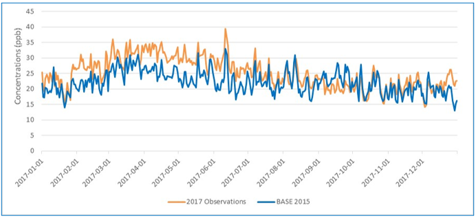
Figure D2 - Text description

Figure D2 shows a time series with a line for modelled 2015 O₃ reference concentrations and a line for observed 2017 O₃ concentrations. The lines represent average daily O₃ concentrations in metropolitan regions across Canada. Concentrations vary between 15 and 40 ppbv approximately, being higher during spring months. The lines show relatively good agreement between observed and modelled O₃ concentrations. However, the modelled O₃ concentrations from January to July were lower than observations. Better agreement was achieved from August to December.

Figure D3 - Text description

Figure D3 shows a time series with a line for modelled 2015 PM_2.5 reference concentrations and a line for observed 2017 concentrations. The lines represent average daily PM_2.5 concentrations in metropolitan regions across Canada. Concentrations vary between 3 and 20 µg/m³ approximately. No clear seasonal trend is visible: modelled concentrations are lower during summer months but this does not coincide with observations. From January to April and from October to December, modelled values are greater than observations, whereas the modelled concentrations are underestimated during the summer months. The lines show better agreement between observed and modelled concentrations during late spring and fall.