
Draft Guidelines for Canadian Drinking Water Quality, Arsenic
Guideline Technical Document for Public Consultation
Consultation period ends: May 6, 2025
Purpose of consultation
This guideline technical document outlines the evaluation of the available information on arsenic with the intent of updating the guideline value for arsenic in drinking water. The purpose of this consultation is to solicit comments on the proposed guideline, on the approach used for its development, and on the potential impacts of implementing it.
The existing guideline technical document on arsenic, developed in 2006, based a maximum acceptable concentration (MAC) of 0.01 mg/L (10 µg/L) on the incidence of internal (lung, bladder and liver) cancers in humans, taking into consideration limitations in municipal- and residential-scale treatment achievability. This document proposes a MAC of 0.005 mg/L (5 µg/L) based on a meta-analysis of epidemiological studies showing evidence of lung cancer from arsenic in drinking water. Lowering the proposed MAC from 10 µg/L to 5 µg/L would lower the estimated excess lifetime risk of lung cancer (above the Canadian background level) from 7 to 3.5 cases in one thousand people. The proposed MAC also considers limitations in municipal- and residential-scale treatment technologies associated with achieving arsenic concentrations in drinking water at or below the health-based value. It is expected that a significant number of water systems across Canada would incur infrastructure, technology and operating costs to meet the proposed guideline, affecting especially small communities with limited resources. Given the health risks of exposure to arsenic, it is recommended that every effort be made to reduce arsenic levels in drinking water to as low as reasonably achievable.
This document is available for a 60-day public consultation period. Please send comments (with rationale, where required) to Health Canada via email: water-consultations-eau@hc-sc.gc.ca
All comments must be received before May 6, 2025. Comments received as part of this consultation will be shared with members of the Federal-Provincial-Territorial Committee on Drinking Water (CDW), along with the name and affiliation of their author. Authors who do not want their name and affiliation shared with CDW members should provide a statement to this effect along with their comments.
It should be noted that this guideline technical document will be revised following the evaluation of comments received, and a drinking water guideline will be established, if required. This document should be considered as a draft for comment only.
Proposed guideline value
A maximum acceptable concentration (MAC) of 0.005 mg/L (5 μg/L) is proposed for arsenic in drinking water based on municipal- and residential-scale treatment achievability. Every effort should be made to maintain arsenic levels in drinking water as low as reasonably achievable (ALARA).
Executive summary
This guideline technical document was prepared in collaboration with the Federal-Provincial-Territorial Committee on Drinking Water (CDW) and assesses all relevant information on arsenic. It assesses the health risks associated with inorganic arsenic in drinking water, taking into account new studies and approaches, as well as the limitations of available treatment technology.
Exposure
Arsenic is a natural element that is widely distributed throughout the Earth's crust. It can enter drinking water sources through the erosion and weathering of soil, minerals and ores, through industrial effluents, mining and smelting processes, through the use of arsenical wood preservation compounds, coal, wood and waste combustion, and through atmospheric deposition.
This guideline technical document considers exposure to inorganic arsenic through ingestion of drinking water.
People in Canada are exposed to arsenic primarily through food and drinking water. The contribution from these two sources depends on the concentration of arsenic in water used for drinking and for reconstituting drinks and/or food. Where a population is living in an area with high levels of naturally occurring arsenic or near a contaminated site, drinking water can be the most important contributor to overall exposure to inorganic forms of arsenic.
Arsenic can be found in both surface water and groundwater sources. An analysis of arsenic concentrations in source waters within Canada revealed localized hotspots with levels exceeding the proposed MAC. Arsenic concentrations are typically higher in groundwater sources than surface waters. Generally, Canadian treated and distributed waters are below the proposed MAC of 5 μg/L.
Health effects
The epidemiological database for inorganic arsenic is extensive. Animal data are of limited use for human risk assessment since animals respond differently to arsenic exposure. Epidemiological studies report associations between oral exposure to arsenic in drinking water and numerous cancer and non-cancer outcomes. The strongest causal relationships for cancer in humans from exposure to arsenic in drinking water at concentrations below 100 µg/L have been demonstrated for the bladder and lungs. Lung cancer is the most sensitive cancer outcome. The proposed MAC for arsenic in drinking water is based on lung cancer in humans; it was calculated by estimating an excess lifetime risk of lung cancer above the Canadian background level. The proposed MAC has been set at a level higher than the level that represents “essentially negligible” risk due to the limitations of the available treatment technology.
Analytical and treatment considerations
The development of a drinking water guideline takes into consideration the ability to both measure the contaminant and remove it from drinking water supplies. Several analytical methods are available for measuring arsenic in water at concentrations well below the proposed MAC. Measurements should be for total arsenic, which includes both the dissolved and particulate forms of arsenic in a water sample.
At the municipal level, treatment technologies that are available to reduce arsenic concentrations in drinking water to below the proposed MAC include coagulation, chemical precipitation, iron removal processes, adsorption, membrane filtration and ion exchange. The performance of these technologies depends on factors such as arsenic species, pH, coagulant type, coagulant dose and type of adsorbent. All of these technologies are better at removing, arsenate [As(V)] than arsenite [As(III)]. Pre-oxidation is recommended if the water contains As(III). Besides treatment, strategies for addressing arsenic include controlled blending prior to system entry points or use of alternative water supplies with no or low arsenic concentrations.
At the residential scale, there are certification standards for devices that rely on filtration, reverse osmosis (RO) or distillation treatment for arsenic reduction. For devices to be certified, the treated As(V) concentration must be less than or equal to 10 μg/L. A review of compiled data from certification of RO devices demonstrates that they consistently remove As(V) to a level of 4 µg /L. It is expected that a treatment device certified for arsenic removal will meet the proposed MAC. However, if the arsenic in treated water still exceeds the proposed MAC, it may indicate that there is As(III) in the water and oxidation of As(III) to As(V) may be required. It is important to consult with a local water specialist to determine the appropriate treatment, including the need for and limitations of an oxidation step.
When using such treatment units, it is important to send samples of water entering and leaving the treatment unit to an accredited laboratory for analysis, to ensure that adequate arsenic removal is occurring. Routine operation and maintenance of treatment units, including replacement of the filter components, should be conducted according to manufacturer specifications.
Distribution system
It is recommended that water treatment systems develop a distribution system management plan to minimize the accumulation and release of co-occurring contaminants, including arsenic. This typically involves minimizing the arsenic concentration entering the distribution system and implementing best practices to maintain stable chemical and biological water quality conditions throughout the system, as well as to minimize physical and hydraulic disturbances.
Application of the guidelines
Note: Specific guidance related to the implementation of drinking water guidelines should be obtained from the appropriate drinking water authority.
All water treatment systems should implement a comprehensive, up-to-date risk management water safety plan. A source-to-tap approach should be taken that ensures water safety is maintained. This approach requires a system assessment to characterize the source water; describe the treatment barriers that prevent or reduce contamination; identify the conditions that can result in contamination; and implement control measures. Operational monitoring is then established and operational/management protocols are instituted (for example, standard operating procedures, corrective actions and incident responses). Compliance monitoring is established and other protocols to validate the water safety plan are implemented (for example, record keeping, consumer satisfaction). Operator training is also required to ensure the effectiveness of the water safety plan at all times.
The guidelines are intended to protect against health effects from exposure to arsenic in drinking water over a lifetime. Any exceedance of the proposed MAC should be investigated and followed by the appropriate corrective actions, if required. For exceedances in source water where there is no treatment in place, additional monitoring to confirm the exceedance should be conducted. If it is confirmed that arsenic concentrations in the water source are above the proposed MAC, then an investigation to determine the most appropriate way to reduce exposure to arsenic should be conducted. This may include the use of an alternate water supply or installation of an arsenic treatment system. Where treatment is already in place and an exceedance occurs, an investigation should be conducted to verify treatment efficacy and to determine whether adjustments are needed to lower the treated water concentration below the proposed MAC.
Discoloration (coloured water) episodes are likely to be accompanied by the release of accumulated contaminants, including arsenic, because dissolved arsenic can adsorb onto deposits in the distribution and plumbing systems. Therefore, discoloured water events should not be considered only an aesthetic issue; they should trigger sampling for metals and possibly distribution system maintenance. However, the absence of discoloured water does not mean that there are no metals being released.
Table of Contents
- 1.0 Exposure considerations
- 2.0 Health considerations
- 3.0 Derivation of the health-based value (HBV)
- 4.0 Analytical methods for detecting arsenic
- 5.0 Treatment considerations
- 6.0 Management strategies
- 7.0 International considerations
- 8.0 Rationale
- 9.0 References
- Appendix A: List of abbreviations
- Appendix B: Anticipated impacts on provinces and territories
- Appendix C: Canadian water quality data
- Appendix D: Primary studies evaluated for risk assessment
- Appendix E: Summary of arsenic removal technologies
1.0 Exposure considerations
1.1 Substance identity
Arsenic is a metalloid with oxidation states of -3, 0, 3 and 5. It is widely distributed throughout the Earth's crust and is a major constituent of at least 245 mineral species. Natural sources of arsenic include volcanically derived sediment, sulphide minerals and metal oxides. The most common arsenic sulphide mineral, globally, is arsenopyrite, which is commonly found in many gold vein deposits, such as those of Yellowknife, Northwest Territories. The most common source of arsenic in Canada is sulphide minerals. These minerals are typically composed of 0.02% to 0.5% arsenic; however, certain pyrite minerals may contain up to 10% arsenic (Hindmarsh and McCurdy, 1986; Abraitis et al., 2004). The properties of select arsenic compounds are presented in Table 1.
| Property | ArsenicTable 1 Footnote a | Calcium arsenateTable 1 Footnote b | Disodium arsenateTable 1 Footnote c | Sodium arseniteTable 1 Footnote d | Arsenic pentoxideTable 1 Footnote e | Arsenic acid (arsenate)Table 1 Footnote e | Arsenic trioxideTable 1 Footnote f |
|---|---|---|---|---|---|---|---|
| CAS RN | 7440-38-2 | 7778-44-1 | 7778-43-0 | 7784-46-5 | 1303-28-2 | 7778-39-4 | 1327-53-3 |
| Molecular formula | As | Ca3(AsO4)2 | Na2HAsO4 | NaAsO2 | As2O5 | AsO(OH)3 | As2O3 |
| Molecular weight (g/mol) | 74.92 | 398.07 | 185.91 | 129.91 | 229.84 | 141.94 | 201.87 |
| Water solubility | Insoluble | 0.13 g/L at 25°C | 610 g/L at 15°C | Freely soluble | 391.9 g/L at 25°C | 590 g/L6 | 582 g/L at 25°C |
| Vapour pressure (volatility) | NA | 0 mm Hg at 20°C (negligible) | NA | NA | 2.81 × 10⁻¹⁰ mm Hg (negligible) | 5.75 × 10⁻¹⁹ mm Hg (negligible) | 4.11 × 10⁻⁹ mm Hg at 25°C (negligible) |
| Octanol-water partition coefficient (Kow) | NA | NA | NA | NA | NA | NA | NA |
| Henry’s Law constant | NA | NA | NA | NA | NA | NA | NA |
CAS RN: Chemical Abstracts Service Registration Number; NA: not applicable
|
|||||||
1.2 Uses, sources and environmental fate
Arsenic-containing compounds are used as alloying agents in the manufacture of transistors, lasers and semi-conductors, as well as in the processing of glass, pigments, textiles, paper, metal adhesives, ceramics, wood treatment/preservatives, ammunition and explosives. The principal sources of arsenic in ambient air are the burning of fossil fuels (especially coal), metal production, agricultural operations and waste incineration. Arsenic is introduced into water through the erosion and weathering of soil, minerals and ores; from industrial and mining effluents; and from atmospheric deposition (Hindmarsh and McCurdy, 1986; Hutton and Symon, 1986; ATSDR, 2007; IARC, 2012). Arsenic naturally occurs in soil but can also enter soil through nonferrous metal mining and smelting, the use of arsenical wood preservation compounds, coal and wood combustion, as well as through waste incineration (ATSDR, 2007).
In surface water, arsenite [As(III)] and arsenate [As(V)] form insoluble salts with cations (usually iron) that can be suspended in the water. These particles generally settle out in sediments. Settling out occurs to a lesser extent in deep groundwater because of higher pH levels and lower iron concentrations (Hindmarsh and McCurdy, 1986).
Arsenic occurs in different forms (organic [or methylated] vs. inorganic) and valences depending upon the pH, microbial activity, and oxidation reduction potential of the water. In well-oxygenated surface waters, As(V) is generally the most common species present (Irgolic, 1982; Cui and Liu, 1988; IARC, 2012); under reducing conditions, such as those often found in deep lake sediments or groundwaters, As(III) is the predominant form (Lemmo et al., 1983; Welch et al., 1988).
Climate change can have impacts on water quality through increased occurrence of extreme events such as floods, droughts and wildfires. General discussions on the impacts of climate change are presented in Berry and Schnitter (2019) and Bush and Lemmen (2019). Fluctuations in groundwater levels due to climate change may have an indirect effect on redox potential. The redox status of the groundwater can be measured by changes in iron, manganese and dissolved oxygen (Jarsjö et al., 2020). Arsenic can be adsorbed to or desorbed from iron or manganese oxyhydroxides as concentrations change in response to changes in aquifer geochemistry (Ayotte et al., 2015; Degnan et al., 2020).
Groundwater levels may rise due to climate change. This may increase contact between the highly conductive topsoil layers and the groundwater. A hydrogeological-geochemical model showed that an increase of 0.2 m in the groundwater level could increase As(III) mass flow by a factor of 1.8. Mass flows of As(III) were shown to be 1 000-fold higher than mass flows of As(V). There is the potential for increased mobility of arsenic when the environment changes from oxidizing to reducing conditions (Jarsjö et al., 2020).
Extensive well pumping and dewatering of groundwater systems has increased arsenic concentrations within aquifers. A study in Perth, Australia determined that no arsenic was present in shallow investigation wells in 1976 (detection limit not provided). After extensive dewatering, arsenic exceeded 1 000 μg/L in monitoring wells, reached up to 7 000 μg/L in uncased boreholes, and was between 5 and 15 μg/L in water supply production wells in 2004 (Appleyard et al., 2006). Higher arsenic concentrations were detected near the water table in the more acidic groundwater zones. Arsenic levels declined with depth (to about 5 m) as the pH of groundwater rose to natural background levels. In deeper wells, redox conditions became progressively more reducing, resulting in the presence of more arsenic. Over-pumping of deeper aquifers leads to the compaction of the surrounding clay, releasing arsenic residing within its pores to the adjacent aquifers (Erban et al., 2013; Smith et al., 2018).
Rainfall events that follow extreme wildfires can impact streams, with effects including increased concentrations of arsenic and dissolved organic carbon (Bladon et al., 2014; Murphy et al., 2015, 2020; Paul et al., 2022; Beyene et al., 2023). Arsenic can be mobilized as a result of wildfire-induced soil disturbances and then enter surface waters and groundwaters. In the United States (U.S.), a study by Pennino et al. (2022) evaluated measured concentrations from the Safe Drinking Water Information System, as well as from the Centers for Disease Control and Prevention (from 2006 to 2016) to explore the impact of wildfires on the contamination of public water systems by several parameters, including arsenic. Arsenic violations (incidents of concentrations above the maximum contaminant level of 0.01 mg/L) associated with groundwater sources increased by 1.08 violations per system over 3 years and by 1.13 violations over 10 years after wildfires compared to the same number of pre-wildfire years. Annual average arsenic concentrations increased by 0.92 μg/L during the three-year pre- vs. post-wildfire time window, and by 0.95 μg/L for the 10-year pre- vs. post-wildfire time window. Overall, the number of arsenic violations post-wildfire were increased for 35% of sites, whereas 48% of sites were observed to have a decreased number of arsenic violations. As for arsenic concentrations, 40% of sites had increased levels and 22% of sites had decreased levels post-wildfire. These data indicate that wildfires are a potential source of arsenic release to groundwater drinking water sources.
1.3 Exposure
People in Canada are exposed to arsenic primarily through food and drinking water. The contribution of these two sources is dependent on the concentration of arsenic in water used for drinking and for reconstituting drinks and/or food. In a situation where a population is living in an area with high levels of naturally occurring arsenic or near a contaminated site, drinking water can be the most important contributor to overall exposure to inorganic forms of arsenic.
Water
Total (inorganic) arsenic data from water monitoring conducted by the provinces and territories (PT) (municipal and non-municipal supplies) were obtained. These datasets included total arsenic concentrations from raw, treated and distribution system waters. Total arsenic concentrations were also obtained from Indigenous Services Canada’s First Nations and Inuit Health Branch (FNIHB) and the National Drinking Water Survey (NDWS). These datasets reflect the different detection limits (DLs) used by accredited laboratories within and among the jurisdictions, as well as their respective monitoring programs. As a result, the statistical analysis of exposure data provides only a limited picture. The results for the PT and FNIHB data are presented in Table 2; for the NDWS in Table 3; and Environment and Climate Change Canada (ECCC) surface water monitoring and PT groundwater monitoring studies are presented in Appendix C. For total arsenic concentrations:
- The PT data typically showed higher arsenic levels in raw groundwater than in surface water. The mean values in treated and distributed water were generally below 5 μg/L, regardless of source.
- The FNIHB data showed mean arsenic values in treated and distributed waters below 5 μg/L. The 90th percentile concentrations were generally below 5 μg/L with some groundwater sources having treated or distributed water that exceeded this value.
- The 90th percentile concentrations in the NDWS data were below 5 μg/L for treated and distributed waters. Higher values occurred in groundwater sources.
- The 90th percentile concentrations in ECCC’s long-term surface water monitoring data were generally below 5 μg/L.
- The PT ambient groundwater monitoring studies (Appendix C) had 90th percentile concentrations as high as 40 μg/L. None of the sources concerned are used for drinking water purposes.
| Jurisdiction (DL μg/L) [years] |
System type | Water type | # Detects /samples | % Detect | Concentration (μg/L) | ||
|---|---|---|---|---|---|---|---|
| Median | MeanTable 2 Footnote a | 90th percentile | |||||
AlbertaTable 2 Footnote 1 (0.07–1) [2014–2018] |
Municipal |
Ground-Raw |
82/90 |
91.1 |
8.05 |
11.10 |
23.50 |
Ground-Treated |
115/131 |
87.8 |
0.70 |
3.65 |
8.59 |
||
Surface-Raw |
148/148 |
100 |
0.40 |
0.59 |
1.00 |
||
Surface-Treated |
552/555 |
99.5 |
0.30 |
0.28 |
0.40 |
||
Ground &/or surface-Treated |
5/6 |
83.3 |
0.45 |
0.37 |
NC |
||
British ColumbiaTable 2 Footnote 2 (0.1–9) [2014–2018] |
Municipal |
Ground-Raw |
136/201 |
67.7 |
1.12 |
18.91 |
5.69 |
Ground-Treated |
0/12 |
0 |
< DL |
< DL |
< DL |
||
Ground-Distribution |
163/216 |
74.5 |
0.735 |
2.54 |
6.43 |
||
Ground-Unspecified |
290/353 |
82.2 |
0.25 |
1.23 |
3.52 |
||
Surface-Raw |
13/68 |
19.1 |
< DL |
0.40 |
0.51 |
||
Surface-Distribution |
15/19 |
78.9 |
0.31 |
1.77 |
5.00 |
||
Surface-Unspecified |
6/90 |
6.67 |
< DL |
0.31 |
< DL |
||
Ground &/or surface-Raw |
6/22 |
27.3 |
< DL |
1.37 |
5.10 |
||
Ground &/or surface-Treated |
18/20 |
90 |
4.075 |
4.35 |
9.08 |
||
Ground &/or surface-Distribution |
38/59 |
64.4 |
0.4 |
2.07 |
6.91 |
||
Ground &/or surface-Unspecified |
23/44 |
52.3 |
0.25 |
1.25 |
4.97 |
||
FNIHB AtlanticTable 2 Footnote 3 (0.1–1.0) |
Public and semi-public |
Ground-Raw |
28/41 |
68.3 |
1.0 |
2.4 |
3.0 |
Ground-Treated |
39/58 |
67.2 |
1.1 |
2.3 |
3.0 |
||
Ground-Distribution |
132/275 |
48 |
< DL |
5.2 |
14.0 |
||
Surface-Raw |
0/9 |
0 |
< DL |
< DL |
< DL |
||
Surface-Treated |
0/19 |
0 |
< DL |
< DL |
< DL |
||
Surface-Distribution |
3/27 |
11.1 |
< DL |
0.6 |
< DL |
||
Private wells and systems |
Ground-Raw |
0/1 |
0 |
< DL |
< DL |
NC |
|
Ground-Distribution |
82/418 |
19.6 |
< DL |
2.1 |
2.4 |
||
FNIHB ManitobaTable 2 Footnote 3 (0.1–1.0) |
Public and semi-public |
Ground-Raw |
138/167 |
8.3 |
< DL |
1.6 |
< DL |
Ground-Treated |
114/160 |
71.3 |
0.5 |
0.8 |
1.6 |
||
Ground-Distribution |
73/187 |
39.0 |
< DL |
1.4 |
2.4 |
||
Surface-Raw |
221/240 |
92.1 |
0.6 |
0.9 |
1.7 |
||
Surface-Treated |
208/243 |
85.6 |
0.4 |
0.6 |
1.0 |
||
Surface-Distribution |
4/6 |
66.7 |
0.5 |
0.5 |
NC |
||
Private wells and systems |
Ground-Raw |
13/13 |
100 |
3.7 |
15.2 |
30.5 |
|
Ground-Treated |
11/19 |
57.9 |
0.5 |
2.7 |
10.8 |
||
Ground-Distribution |
338/816 |
41.4 |
< DL |
1.6 |
3.1 |
||
FNIHB OntarioTable 2 Footnote 3 (0.1–0.6) |
Public and semi-public |
Ground-Raw |
2/36 |
5.6 |
< DL |
0.9 |
< DL |
Ground-Treated |
36/258 |
14.0 |
< DL |
0.9 |
2.5 |
||
Ground-Distribution |
34/201 |
16.9 |
< DL |
1.0 |
2.0 |
||
Surface-Raw |
4/60 |
6.7 |
< DL |
0.7 |
< DL |
||
Surface-Treated |
14/391 |
3.6 |
< DL |
0.5 |
< DL |
||
Surface-Distribution |
1/40 |
2.5 |
< DL |
0.5 |
< DL |
||
Private wells and systems |
Ground-Raw |
1/2 |
50 |
0.3 |
0.3 |
NC |
|
Ground-Treated |
1/7 |
14.3 |
< DL |
0.4 |
NC |
||
Ground-Distribution |
17/372 |
4.6 |
< DL |
0.6 |
< DL |
||
ManitobaTable 2 Footnote 4 (0.1–2) [2011–2018] |
Municipal |
Ground-Raw |
697/799 |
87.2 |
1.33 |
4.54 |
10.70 |
Ground-Treated |
980/1 179 |
83.1 |
0.87 |
2.38 |
6.41 |
||
Ground-Distribution |
88/100 |
88 |
0.94 |
2.33 |
6.07 |
||
Surface-Raw |
601/609 |
98.7 |
1.01 |
1.97 |
5.10 |
||
Surface-Treated |
613/643 |
95.3 |
0.70 |
0.84 |
1.42 |
||
Surface-Distribution |
69/74 |
93.2 |
0.76 |
0.79 |
1.20 |
||
Ground &/or surface-Raw |
172/179 |
96.1 |
1.60 |
2.89 |
5.64 |
||
Ground &/or surface-Treated |
180/208 |
86.5 |
0.70 |
1.57 |
4.41 |
||
Ground &/or surface-Distribution |
24/26 |
92.3 |
0.72 |
1.12 |
3.41 |
||
New BrunswickTable 2 Footnote 5 (1–2) [2013–2018] |
Municipal |
Ground-Raw |
347/1 222 |
28.4 |
< DL |
1.84 |
4.00 |
Ground-Treated |
76/199 |
38.2 |
< DL |
7.22 |
10.0 |
||
Ground-Distribution |
95/627 |
15.2 |
< DL |
1.1 |
2.0 |
||
Ground-Unspecified |
20/88 |
22.7 |
< DL |
1.0 |
2.0 |
||
Surface-Raw |
0/60 |
0 |
< DL |
< DL |
< DL |
||
Surface-Distribution |
1/186 |
0.5 |
< DL |
0.59 |
< DL |
||
Ground & surface-Raw |
76/301 |
25.3 |
< DL |
0.91 |
1.8 |
||
Ground & surface-Treated |
326/761 |
42.8 |
< DL |
10.9 |
4.0 |
||
Ground & surface-Distribution |
95/685 |
13.9 |
< DL |
1.0 |
1.0 |
||
Ground & surface-Unspecified |
23/79 |
29.1 |
< DL |
4.6 |
3.0 |
||
NewfoundlandTable 2 Footnote 6 (0.5) [2014–2018] |
Municipal |
Ground-Raw |
28/99 |
28.3 |
< DL |
1.45 |
3.00 |
Ground-Distribution |
527/1 216 |
43.3 |
< DL |
2.04 |
5.00 |
||
Surface-Raw |
9/627 |
1.4 |
< DL |
0.51 |
< DL |
||
Surface-Distribution |
37/3 223 |
1.1 |
< DL |
0.51 |
< DL |
||
Nova ScotiaTable 2 Footnote 7 (1–2) [2011–2018] |
Municipal |
Ground-Raw |
89/245 |
36.3 |
< DL |
2.34 |
5.00 |
Ground-Treated |
43/124 |
34.7 |
< DL |
1.43 |
3.60 |
||
Surface-Raw |
148/148 |
100 |
0.40 |
0.59 |
1.00 |
||
Surface-Treated |
543/546 |
99.5 |
0.30 |
0.28 |
0.40 |
||
OntarioTable 2 Footnote 8 (0.11) [2013–2018] |
Municipal |
Ground-Raw |
556/563 |
98.8 |
0.40 |
0.77 |
1.40 |
Ground-Treated |
222/233 |
95.3 |
0.50 |
0.65 |
1.36 |
||
Ground-Distribution |
141/146 |
96.6 |
0.40 |
0.55 |
1.10 |
||
Surface-Raw |
248/249 |
99.6 |
0.50 |
0.61 |
1.00 |
||
Surface-Treated |
241/250 |
96.4 |
0.30 |
0.35 |
0.59 |
||
Surface-Distribution |
288/293 |
98.3 |
0.30 |
0.38 |
0.60 |
||
Ground &/or surface-Raw |
485/527 |
92.0 |
0.60 |
0.73 |
1.20 |
||
Ground &/or surface-Treated |
544/560 |
97.1 |
0.40 |
0.54 |
1.00 |
||
Ground &/or surface- Distribution |
597/622 |
96.0 |
0.40 |
0.50 |
0.90 |
||
Prince Edward IslandTable 2 Footnote 9 (0.1–4) [2015–2018] and [2018–2023] |
Municipal |
Ground-Raw |
NP |
NP |
NP |
1.4 |
NP |
Ground-Distribution |
NP |
NP |
NP |
0.7 |
NP |
||
Semi-public |
Ground-Unspecified |
NP |
NP |
NP |
1.8 |
NP |
|
Private wells [2018–2023] |
Ground-RawTable 2 Footnote b |
10 741/ 10 982 |
97.8% |
0.7 |
1.4 |
2.8 |
|
QuebecTable 2 Footnote 10 (0.3–20) [2013-2018] |
Municipal |
Ground-Distribution |
1 440/ 6 814 |
21.1 |
< DL |
1.4 |
3 |
Surface-Distribution |
202/2 171 |
9.3 |
< DL |
0.71 |
< DL |
||
SaskatchewanTable 2 Footnote 11 (0.01–0.5) |
Municipal [2013–2018] |
Ground-Raw |
196/218 |
89.9 |
3.80 |
10.21 |
28.21 |
Surface-Raw |
83/83 |
100 |
1.50 |
3.67 |
10.22 |
||
Ground & surface-Treated |
151/176 |
85.8 |
1.10 |
3.37 |
10.66 |
||
Ground & surface-Distribution |
2 255/ 2 528 |
89.2 |
0.80 |
3.1 |
8.4 |
||
Private wells [1996–2011] |
Ground-Raw |
3 319/ 4 128 |
80.4 |
0.9 |
5.0 |
14.0 |
|
YukonTable 2 Footnote 12 (0.1–4.3) [2014–2018] |
Non-municipal |
Ground-Unspecified |
27/30 |
90 |
0.63 |
3.97 |
14.52 |
Municipal |
Ground-Raw |
179/183 |
97.8 |
2.1 |
4.5 |
14.1 |
|
Ground-Treated |
102/125 |
81.6 |
0.60 |
1.8 |
5.4 |
||
Surface-Raw |
9/9 |
100 |
14.7 |
13.3 |
16.0 |
||
Surface-Treated |
20/21 |
95.2 |
2.0 |
2.6 |
6.8 |
||
CanadaTable 2 Footnote c |
Municipal |
Ground-Treated |
1 537/ 2 002 |
76.8 |
NA |
2.6 |
NA |
Ground-Distribution |
2 454/ 9 118 |
26.9 |
NA |
1.5 |
NA |
||
Surface-Treated |
1 426/ 1 682 |
84.8 |
NA |
0.60 |
NA |
||
Surface-Distribution |
612/5 966 |
10.3 |
NA |
0.5 |
NA |
||
Ground &/or Surface-Treated |
1 224/ 1 731 |
70.7 |
NA |
5.5 |
NA |
||
Ground &/or Surface-Distribution |
3 899/ 3 920 |
99.5 |
NA |
2.28 |
NA |
||
DL: detection limit; < DL: below detection limit (for median with < 50% detects; for 90th percentile with < 10% detects and mean with 0% detects); FNIHB: First Nations and Inuit Health Branch; NA: not applicable; NC: not calculated due to insufficient sample size; NP: not provided; Unspecified: sample not specified whether raw, treated or distribution.
|
|||||||
| Water type | Summer (μg/L) | Winter (μg/L) | ||||||
|---|---|---|---|---|---|---|---|---|
| Detects/ samples | Median | MeanTable 3 Footnote a | 90th percentile | Detects/ samples | Median | MeanTable 3 Footnote a | 90th percentile | |
| Well-Raw | 7/18 | < DL | 2.36 | 9.30 | 7/17 | < DL | 0.80 | 2.00 |
| Well-Treated | 5/18 | < DL | 1.58 | 4.40 | 4/16 | < DL | 1.50 | 4.90 |
| Well- Distribution | 6/18 | < DL | 1.61 | 4.30 | 2/9 | < DL | 1.50 | NC |
| Lake-Raw | 0/21 | < DL | < DL | < DL | 1/20 | < DL | 0.58 | < DL |
| Lake-Treated | 0/21 | < DL | < DL | < DL | 0/20 | < DL | < DL | < DL |
| Lake-Distribution | 0/21 | < DL | < DL | < DL | 1/11 | < DL | 0.57 | < DL |
| River-Raw | 3/26 | < DL | 1.25 | 4.90 | 3/22 | < DL | 0.80 | 2.00 |
| River-Treated | 0/25 | < DL | < DL | < DL | 0/22 | < DL | < DL | < DL |
| River-Distribution | 0/26 | < DL | < DL | < DL | 0/12 | < DL | < DL | < DL |
DL: detection limit (0.5 μg/L); < DL: below detection limit (for median with < 50% detects; for 90th percentile with < 10% detects and mean with 0% detects); NC: not calculated due to insufficient data.
Source: Health Canada, 2017. |
||||||||
A First Nations Food, Nutrition and Environments Study included results from eight Assembly of First Nation regions (FNFNES, 2021). The document includes a summary of tap water sampling from 1 516 households. Arsenic concentrations were below 10 μg/L in all households except for one, which had a maximum arsenic concentration of 14 μg/L.
A review of publicly available arsenic concentrations in Canadian drinking water was carried out by McGuigan et al. (2010). Any information that could be found within the literature (raw, treated arsenic concentrations and reports) was compiled. This study showed that most water samples had arsenic concentrations below 10 μg/L. There are several localized hot spots within Alberta, British Columbia, New Brunswick, Newfoundland and Labrador, Nova Scotia, Quebec and Saskatchewan with higher arsenic concentrations.
Food
Food is generally considered one of the most important sources of arsenic exposure in Canada. The exception to this is in populations living in areas of high levels of naturally occurring arsenic or near a contaminated site. Considering average exposures to arsenic from food (Health Canada, 2022a), food represents the largest exposure source when arsenic levels in water are below 3 µg/L for infants and below 5 µg/L for adults; above these concentrations, drinking water becomes the primary source of exposure. Arsenic can exist in both organic and inorganic forms in food; the inorganic forms are widely considered to be much more toxic to humans. The amount and forms of arsenic found in foods are dependent on several factors such as food type, growing conditions and processing techniques (CFIA, 2022a). The Canadian Total Diet Study is a food surveillance program that monitors the concentrations of chemical contaminants in foods that are typically consumed by people in Canada. Overall, from 1993 to 2018, detected concentrations of arsenic ranged from as low as 0.0075 ng/g in tap water to as high as 8 495 ng/g in marine fish. Arsenic concentrations for different foods ranged from 0.7 to 6.6 ng/g in apple juice, 219 to 362 ng/g in shellfish, 3 215 to 8 495 ng/g in marine fish, 120 to 1 087 ng/g in freshwater fish, 31 to 99 ng/g in white rice and non-detectable (ND) to 2.6 ng/g in infant formula. In tap water, arsenic concentrations ranged from ND to 1.05 ng/g (Health Canada, 2020a).
Health Canada has established maximum levels (MLs) for total arsenic in beverages (0.1 ppm) except fruit juices and nectars, and in bottled water (0.01 ppm), as well as for inorganic arsenic in fruit juices and nectars (0.01 ppm), and in grape juices and nectars (0.03 ppm) (Health Canada, 2020b).
Rice is considered an important dietary source of exposure and is likely to have higher arsenic concentrations compared to other foods because it is grown under flooded conditions. Inorganic arsenic can represent approximately 70% of the arsenic content in rice and it is highly bioavailable. Levels in brown rice (which is less processed) are generally higher than in white rice. Survey results collected by the Canadian Food Inspection Agency (CFIA) from 2011 to 2013 indicate an average inorganic arsenic concentration of 94.19 ppb in rice and rice products (CFIA, 2018a). Health Canada has established MLs of 0.2, 0.35 and 0.1 parts per million (ppm) for inorganic arsenic in polished (white) rice, husked (brown) rice and rice-based foods for infants, respectively. These MLs also apply to white and brown rice when used as an ingredient in other foods (Health Canada, 2020b).
Total arsenic was measured in children’s food samples as part of the 2013 to 2014 Children’s Food Project conducted by the CFIA. Total arsenic was detected in 20.6% of samples with concentrations ranging from 0.005 ppm in samples of juice and purees containing meat to a maximum of 0.023 ppm in a pureed vegetable sample. There were two samples of juice that tested positive for arsenic, one pear juice (0.0067 ppm) and one apple juice (0.0054 ppm). Both samples had an inorganic arsenic level below the ML of 0.01 ppm in fruit juices. The total arsenic concentrations reported in samples collected over this period were all below or within the ranges reported for previous periods (2008 to 2009 and 2010 to 2011) (CFIA, 2018b). The CFIA has also published targeted surveys of total arsenic and arsenic speciation in alcoholic beverages, fish, shellfish and crustaceans sampled during the 2018 to 2019 period and added rice-based infant foods to its surveys during the 2019 to 2020 period. The average total arsenic (and total inorganic) concentrations reported are shown in Table 4.
| Food samples | Average total arsenic (total inorganic arsenic) in ppb | |
|---|---|---|
| 2018 to 2019 | 2019 to 2020 | |
| Alcoholic beverages | 3.31 (3.12) | 4.28 (2.18) |
| Fish | 1 027 (1.31) | 1 528 (1.48) |
| Shellfish and crustaceans | 5 831 (34.28) | 4 810 (23.08) |
| Rice-based infant food | N/A | 78.09 (52.91) |
| N/A: not available; ppb: parts per billion. | ||
In a Chemicals Management Plan Monitoring and Surveillance Fund project entitled “Surveillance of Arsenic Speciation in Various Food Samples,” which was led by the Health Products and Foods Branch of Health Canada, 71 samples from the 2011 Total Diet Study and 75 samples from the 2012 study were analyzed for six arsenic species: arsenobetaine, arsenocholine, dimethylarsenic acid (DMA), monomethylarsenic acid (MMA), As(III) and As(V). Arsenobetaine and arsenocholine were mainly found in meat, fish and mushroom samples, with these two species representing a large portion of total arsenic in fish (greater than 95% of total arsenic). For the meat or processed food samples, 35 samples contained these two arsenic species and, together, they accounted for less than 13% (average) of total arsenic. DMA and MMA were detected in most food samples, with As(III) and As(V) being the most predominant species measured. For the 2011 and 2012 Total Diet Study samples, total arsenic concentrations ranged from 2.86 (cherries) to 80.9 (rice-based cereal) ng/g and 0.36 (coffee) to 72.9 (herbs and spice) ng/g, respectively (Health Canada, 2016).
Air
The National Air Pollution Surveillance program measured ambient arsenic air concentrations associated with fine particulate matter (PM2.5) across 16 stations in Canada over the 2009 to 2013 period. An average concentration of 0.0009 µg/m3 was reported, with a range of less than 0.000016 to 0.74 µg/m3 for 4 128 samples (Galarneau et al., 2016). Individuals residing near point sources of inorganic arsenic, such as lead and copper smelters, may be exposed to levels that are much higher than those to which the general population is exposed. The Environment Canada and Health and Welfare Canada (1993) Priority Substances List assessment report states that air concentrations of arsenic near smelters and a gold ore roaster ranged from 0.086 to 0.3 µg/m3, whereas the mean arsenic level (within most of the 11 cities investigated) was 0.001 µg/m3. In Rouyn-Noranda, Quebec, in the vicinity of a copper smelter, annual average concentrations of arsenic in ambient air generally showed a downward trend from the early 1990s to 2021. Differences in the magnitude of arsenic concentrations are observed depending on the location of the monitors: stations that are farther away from the smelter show lower annual concentrations than stations closer to the facility. Data from 1993 up to 2005 indicate substantially higher annual average arsenic concentrations, often surpassing 500 ng/m3 and reaching up to 968 ng/m3 at the stations nearest to the facility. By contrast, concentrations ranged from 60 to 260 ng/m3 at stations farther away during the same time period. From 2005 to 2021, annual average arsenic concentrations typically ranged from 70 to 200 ng/m3 at the stations adjacent to the smelter, from 16 to 73 ng/m3 at stations 500 to 600 m away, and from 3 to 39 ng/m3 at stations farther away.
Fine particulate matter in outdoor air, including metal compounds bound to particles, can infiltrate into the indoor environment and negatively affect indoor air quality. There is evidence that infiltrated particles reflect their outdoor origin in terms of elemental composition, and that particulate matter (PM) can settle as dust in the indoor environment (Rasmussen et al., 2018). Hence, there is the potential for PM originating from outdoor sources to impact health through deterioration of indoor air quality. Arsenic in indoor dust from 1 025 urban homes in 13 Canadian cities was measured as part of an evaluation of nationally representative concentrations, loads and loading rates for several metals in urban homes. Arsenic levels ranged from 0.1 to 153 µg/g, with a mean reported level of 13.1 µg/g and a 95th percentile level of 40.6 µg/g. Approximately half of the homes in the study were located within 2 kilometres of industrial zones and were characterized by higher dust and metal loading rates compared to homes in non-industrial zones. However, no significant difference in dust metal concentrations (including arsenic) was observed between non-industrial and industrial zones. The authors indicate that the higher dust loading rate in the industrial zone is likely the driver for the higher metal loading rates observed in the homes located near industrial zones (Rasmussen et al., 2013).
Soil
Arsenic in soil (predominantly inorganic) originates from underlying materials that form soils, industrial wastes or the use of arsenical wood preservation compounds. In general, exposure to arsenic from soil can be expected to occur only in areas with industrial and geological sources. Children are potentially more exposed to arsenic from soil through incidental ingestion. In a recent Canadian study, the mean arsenic concentration in background soil (parent material below the surface soil known as the C horizon) at 532 sites in 10 provinces was 6.2 mg/kg for both surface layer (0 to 5 cm) and C horizon soils combined. Elevated concentrations were found in Nova Scotia (mean: 10 mg/kg; standard deviation [SD]: 28.1 mg/kg; 95th percentile: 28 mg/kg, 67 samples), New Brunswick (mean: 8.5 mg/kg; SD: 5.4 mg/kg; 95th percentile: 21 mg/kg, 115 samples) and Newfoundland and Labrador (mean: 9.7 mg/kg; SD: 0.11 mg/kg; 95th percentile: 31 mg/kg, 66 samples). Overall, significantly lower arsenic concentrations were detected in the surface layer (median 4.7 mg/kg) compared to the C horizon (median 6.3 mg/kg), which suggests that most of the arsenic variability across regions may be due to the bedrock characteristics (namely, natural weathering of arsenic-rich parent materials) (Dodd et al., 2017).
Significantly higher levels of arsenic can be found in areas influenced by natural geological sources or mining operations. In tailings from mining operations in 14 historical gold districts in Nova Scotia, arsenic concentrations ranged from 10 to 312 000 mg/kg (mean: 11 900 mg/kg, 482 samples) (Parsons et al., 2012). In the Yellowknife area, the concentration of arsenic in the top soil layer (0 to 5 cm) was estimated to range from less than 2 to 4 700 mg/kg (median = 120 mg/kg) within 30 km of Yellowknife. Within 20 km of Yellowknife, 95% of the upper 5 cm layer samples exceeded the Canadian Council of Ministers of the Environment (CCME) guideline for residential soils (12 mg/kg), whereas only 49% of soils beyond 20 km exceeded this value. High concentrations of arsenic (up to 4 700 mg/kg) were measured in publicly accessible soils near decommissioned mine roaster stacks in the region. The authors estimated the geochemical background range of arsenic for the region as 0.25 to 15 mg/kg based on 1 490 samples of till, excluding any samples collected within 20 km of the Yellowknife area due to the influence of historic mining. The 95th percentile level was estimated to be below 22 mg/kg (Palmer et al., 2021).
Consumer products
Tobacco contains measurable levels of arsenic. Tobacco is grown in over 120 countries and levels of arsenic in tobacco vary with geographical region (Lugon-Moulin et al., 2008). China and the U.S. are the largest producers of tobacco leaves in the world (Eriksen et al., 2012). A recent study estimated a mean value of 0.29 mg/kg (SD 0.04) for arsenic in tobacco extracted from 50 samples of popular U.S. cigarette brands (Fresquez et al., 2013), whereas the mean for 47 samples of popular cigarette brands in China was 0.85 mg/kg (SD 0.73) (O’Connor et al., 2010). Campbell et al. (2014) analyzed 14 samples of tobacco from the United Kingdom, U.S. and China, including certified reference materials and cigarette products. The concentrations of total inorganic arsenic species ranged from 144 to 3 914 μg/kg, while DMA ranged from 21 to 176 μg/kg, and MMA ranged from 30 to 116 μg/kg. Overall the data indicated a consistent ratio of approximately 4:1 for inorganic arsenic versus the organic forms.
Cannabis may also be a potential source of exposure to arsenic although research on arsenic levels in cannabis products is very limited. A study by Bengyella et al. (2022) indicates that arsenic accumulates in the roots, stems and leaves of eight different varieties of hemp plants. The levels varied widely between plant varieties and plant structures, ranging from less than 2 ppm to greater than 12 ppm. Further research is required to understand the potential for exposure to arsenic from cannabis consumption.
Biomonitoring data
The Canadian Health Measures Survey (CHMS) is a national survey which collects information from people in Canada (from 10 provinces) about their general health. The CHMS is the most comprehensive, direct health measures survey conducted in Canada and is designed to represent the population of people in Canada. The survey provides baseline data on several indicators of health including environmental exposures to chemicals such as arsenic. These biomonitoring data reflect all routes of exposure.
Exposure to inorganic arsenic can be estimated from the sum of urinary concentrations of two inorganic species, As(III) and As(V), and their methylated (organic) metabolites, MMA and DMA. While urinary MMA and DMA may also be derived directly from consumption of several food items containing MMA or DMA, or through human metabolism of the organic arsenic compounds aresnosugars and aresenolipids which are contained in seafood, the sum of the urinary concentrations of As(III), As(V), MMA and DMA is known to provide a more stable estimate of inorganic arsenic exposure than any of the individual species, given that population variations in degree of methylation due to factors such age, gender, body mass index (BMI), etc. have been shown not to influence the sum (Hays et al., 2010).
Sampling for inorganic-related arsenic species (As(III), As(V), MMA and DMA) in urine spans over five CHMS cycles from 2009 to 2019 (Health Canada, 2021a). The geometric mean concentrations of inorganic arsenic (calculated as the sum of inorganic-related arsenic species) in urine for all age groups (ages 3 to 79) in the Canadian population remained relatively unchanged over the five cycles of sampling, ranging from 5.1 to 5.5 µg arsenic/L. Urinary inorganic arsenic concentrations by age and sex over the five cycles are shown in Table 5. The biomonitoring component of the CHMS provides a snapshot of population exposure (to inorganic arsenic) integrated from all sources. Inorganic arsenic concentrations in urine from the CHMS 2016 to 2017 (Faure et al., 2020) and 2018 to 2019 (report to be published) were compared to a level in urine equivalent to a health-based exposure guidance value (biomonitoring equivalent). The biomonitoring equivalent for arsenic in urine used for comparison is 6.4 µg arsenic/L, which was derived from a reference dose of 0.0003 mg/kg body weight per day based on hyperpigmentation, keratosis and possible vascular complications. The resultant hazard quotient, calculated as the ratio of population level concentrations to the biomonitoring equivalent, exceeded 1 at the 95th percentile of population concentrations. However, it did not exceed 1 when the geometric mean of population level concentrations was used, which suggests that exposure may exceed existing guidance values for a portion of the population, at least on an intermittent basis.
| Age group (years) or sex | Range of urinary inorganic arsenic concentrations (geometric mean) (µg/L) |
|---|---|
| 3 to 5 | 5.0 to 5.7 |
| 6 to 11 | 5.1 to 6.4 |
| 12 to 19 | 5.1 to 6.0 |
| 20 to 39 | 5.2 to 6.2 |
| 40 to 59 | 4.9 to 5.3 |
| 60 to 79 | 4.6 to 5.4 |
| Males | 5.0 to 6.1 |
| Females | 5.0 to 5.2 |
The Maternal-Infant Research on Environmental Chemicals (MIREC) study is a national prospective biomonitoring study involving pregnant women and pregnant people aged 18 and older recruited from 10 cities across Canada between 2008 and 2011 (Arbuckle et al., 2013). Total arsenic was measured in mothers’ blood in the first and third trimester as well as in umbilical cord blood and meconium. Detection rates were highest in the first trimester blood (92.5%) and lowest in meconium (6.1%). Total arsenic in first trimester whole blood samples (n = 1 938) had geometric mean, 95th percentile and maximum levels of 0.75 µg/L, 2.32 µg/L and 34.46 µg/L, respectively (Ettinger et al., 2017). Additionally, speciated arsenic was measured in first trimester urine (n = 1 933); however, only DMA was commonly detected with geometric mean, 95th percentile and maximum levels of 2.30 µg/L, 11.99 µg /L and 64.42 µg /L, respectively. First and third trimester total blood arsenic concentrations and urinary DMA concentrations were higher in women who were older, foreign-born or had a higher education level. Positive and statistically significant relationships between both first trimester total blood arsenic and maternal DMA levels and gestational diabetes were also observed in this cohort (Shapiro et al., 2015; Ashley-Martin et al., 2018). First trimester total blood arsenic concentrations were also associated with an increased risk of gestational hypertension and preeclampsia in MIREC participants. Individuals with higher manganese levels were less prone to the adverse effect of arsenic on gestational hypertension (Borghese et al., 2023). Additional data are available for total arsenic in blood samples from children aged 2 to 5 from a follow-up child development study (MIREC-CD Plus). Median and maximum levels of total arsenic in whole blood samples from children (n = 449) were 0.464 µg/L and 20.7 µg/L, respectively (Ashley-Martin et al., 2019). No associations were found between childhood exposures to arsenic and anthropometric measures (for example, BMI). In a follow-up study of MIREC (MIREC-ENDO, 2018 to 2021) participants aged 7 to 9, arsenic concentrations in whole blood were detected in 48% and 55% of male and female children, respectively; median concentrations were 0.23 µg/L in males and 0.38 µg/L in females (unpublished data). Total blood arsenic was measured in mothers of these children at the same time (7–9 years postpartum); median concentrations of 2.30 µg/L and 95% percentiles of 0.38 µg/L were detected in 97% of mothers (unpublished data).
2.0 Health considerations
2.1 Kinetics
2.1.1 Absorption
Most inorganic arsenic compounds are well absorbed (> 80%) from the gastrointestinal tract; however, absorption decreases with decreasing solubility (IARC, 2012). Both MMA and DMA are also well absorbed following oral ingestion (approximately 75% to 85%) (ATSDR, 2007). Absorption through inhalation occurs to a lesser extent than absorption through ingestion; however, increased solubility and decreasing particle size can increase absorption. Large airborne particulates containing arsenic that enter the upper respiratory tract may also be absorbed in the intestine if later swallowed. Both organic and inorganic arsenic are poorly absorbed by the skin and thus this route of exposure is of minor importance compared to ingestion (U.S. NRC, 1999; ATSDR, 2007, 2016; IARC, 2012).
The movement of As(III) across human cells is facilitated by aquaglyceroporins (AQPs) and hexose permeases (IARC, 2012; Mukhopadhyay et al., 2014). Whereas AQP9 is found in astrocytes and liver cells, AQP7 is found in the kidney, adipose tissue and the testis (Kageyama et al., 2001). Liu et al. (2002) reported that As(III) is transported into cells by aquaglyceroporins AQP7 and AQP9, which also transport water and glycerol into cells. APQ9 also transports monomethylarsenite (MMAIII) at a rate nearly 3 times faster than As(III) (Liu et al. 2006). Studies have suggested that the transport of As(V), on the other hand, occurs via phosphate transporters since it is chemically similar to phosphate (Huang and Lee, 1996; Cohen et al., 2013; Garbinski et al., 2019).
2.1.2 Distribution
Once ingested, inorganic arsenic appears rapidly in the bloodstream, where it binds primarily to hemoglobin (Axelson, 1980). Correlations have been reported between increasing levels of inorganic arsenic in drinking water and arsenic levels in blood (Arikan et al., 2015; Rodrigues et al., 2015). In the blood, inorganic arsenic species can bind to the sulfhydryl groups of proteins and low molecular weight compounds such as glutathione and cysteine (U.S. NRC, 1999). Persistence in the blood depends on the binding and transport characteristics of the arsenic species. For example, As(III) has an approximate 5- to 10-fold greater affinity for sulfhydryl groups than As(V), which may explain the lower cellular uptake and tissue concentrations of the pentavalent forms (Jacobson-Kram and Montalbano, 1985).
Within 24 hours of oral exposure, arsenic is found mainly in the liver, kidneys, lungs, spleen and skin (Wickström, 1972). Skin, bone and muscle represent the major storage organs. The accumulation of arsenic in skin, for example, is likely attributable to the abundance of proteins containing sulfhydryl groups (Fowler et al., 2007). As(III) transport throughout the human body is reportedly linked to glucose permease which is reported to be highly expressed in heart and brain cells (Garbinski et al., 2019). Transplacental transfer of arsenic in humans has also been reported to occur (Amaya et al., 2013).
Ingested organic arsenic species, such as monomethylarsonic acid (MMAV) and dimethylarsinic acid (DMAV), are not readily taken up by cells and are largely excreted unchanged (Cohen et al., 2006). Animal studies, however, have shown that direct acute exposure to MMA and DMA resulted in some distribution to the bladder, kidneys, lungs and blood (ATSDR, 2007).
Overall, the distribution and retention of arsenic is influenced by many factors including the chemical species, dose level, tissue type, methylation capacity, valence state and route of administration (Thomas et al., 2001).
2.1.3 Metabolism
In humans, ingested arsenic is metabolized mainly in the liver via enzymatic biotransformation by arsenite methyltransferase (AS3MT) into methylarsenite and dimethylarsenite. The methylation of arsenic occurs through alternating steps of reduction and oxidative methylation, with the trivalent species serving as the methyl substrate and S-adenosylmethionine as the methyl donor co-substrate. The sequential reduction and methylation of arsenic compounds result in the creation of pentavalent MMAV and DMAV, as well as the trivalent monomethylarsonous acid (MMAIII) and dimethylarsinous acid (DMAIII) (U.S. NRC, 2001; Vahter and Concha, 2001). An alternative methylation pathway exists in animals whereby trivalent arsenic conjugates with glutathione (which catalyses methyl transfer), creating thiol-bound trivalent arsenicals which serve as substrates for AS3MT-catalyzed methylation (IPCS, 2001; EFSA, 2009; Watanabe and Hirano, 2013; Cullen, 2014).
Genetic polymorphisms in enzymes associated with methylation can lead to increased total arsenic retention time in the body, with greater elimination of inorganic arsenic and MMA and reduced elimination of DMA. Amino acid substitutions in the AS3MT enzymes can decrease methylation activity by decreasing substrate affinity and thereby lowering the overall rates of catalysis and stability. Individuals with such polymorphisms may have an increased risk for arsenic-related diseases (Li et al., 2017). Genetic polymorphisms in other enzymes, such as glutathione S-transferase omega 1, methylenetetrahydrofolate reductase (Ahsan et al., 2007; Lindberg et al., 2007; Luo et al., 2018) and formiminotransferase cyclodeaminase (Pierce et al., 2019), have also been associated with altered cancer risk; however, the risk appears weaker compared to that for polymorphisms in AS3MT enzymes (Chung et al., 2010; Gao et al., 2015). Additional factors that can influence inorganic arsenic methylation include age, sex, ethnicity, dose level, pregnancy and nutrition (see section 2.2.2).
Unlike inorganic arsenic, ingested organic arsenicals such as MMAV and DMAV undergo very little biotransformation and are excreted almost entirely unchanged; therefore, ingestion of organic forms of arsenic do not produce as much of the highly reactive trivalent arsenicals that are cytotoxic and genotoxic (Cohen et al., 2006).
2.1.4 Elimination
As(III) tends to accumulate in tissues; however, As(V) and organic arsenic are rapidly and almost completely eliminated via the kidneys (Bertolero et al., 1987). DMA appears to be more readily excreted than MMA (U.S. NRC, 2001). In humans, the relative proportions of arsenic species in the urine are usually about 10% to 30% inorganic arsenic, 10% to 20% MMA and 60% to 70% DMA (Vahter, 2000; Caldwell et al., 2009). Christian et al. (2006) reported that pregnant women and pregnant people exposed to elevated levels of inorganic arsenic through drinking water excreted ingested arsenic mostly as DMA (79% to 85%) with lesser amounts excreted as inorganic arsenic (8% to 16%) and MMA (5% to 6%). Siblings and parents reportedly show similar patterns of arsenic methylation in urine, which suggests that the metabolism of inorganic arsenic may be genetically influenced (Chung et al., 2002).
There appear to be two main processes, with different rates, for the elimination of ingested As(III) from the body (Lovell and Farmer, 1985). The first is the rapid urinary excretion of inorganic arsenic in both the trivalent and pentavalent forms (close to 90% of the total urinary arsenic over the first 12-hour period). The second involves the sequential methylation of As(III) in the liver to the organic forms MMAIII, DMAIII, MMAV and DMAV (Buchet and Lauwerys, 1985; Lovell and Farmer, 1985). Excretion of the methylated compounds commences approximately 5 hours after ingestion but reaches its maximum level 2 to 3 days later. Less important routes of elimination of inorganic arsenic include skin, hair, nails, sweat and breast milk (ICRP, 1975; Concha et al., 1998; Kurttio et al., 1999). The half-life of inorganic arsenic in humans is estimated to be between 2 and 40 days (Pomroy et al., 1980).
Bile also serves as a major route of arsenic detoxification whereby excess arsenic in the liver is pumped out as an arsenic-glutathione complex (both inorganic and methylated forms) through a specific adenosine triphosphate binding cassette transporter known as multi-drug resistance-associated protein (Leslie, 2011; Garbinski et al., 2019).
2.1.5 Physiologically based pharmacokinetic modelling
Physiologically based pharmacokinetic (PBPK) models for inorganic arsenic have been developed for both animals and humans (Mann et al., 1996a,b; Yu, 1999; Gentry et al., 2004; El-Masri and Kenyon, 2008; El-Masri et al., 2018). These models were developed for predicting urinary and fecal elimination of arsenic and metabolites by using species-specific blood flow and tissue volume parameters (considering age) as well as tissue metabolic considerations (namely linear, first-order or saturable Michaelis-Menten).
Much of the scientific literature on the mechanisms of arsenic toxicity suggests that the trivalent forms (As(III), MMAIII and DMAIII) are likely responsible. However, it is still unclear which forms of arsenic are responsible for the tissue responses that lead to cancer and non-cancer outcomes. In addition, the enzymes involved in tissue oxidation of trivalent species and the transfer processes involved in transporting trivalent species from tissues to blood and then to urine are not fully understood. Currently available PBPK models describe the appearance of trivalent arsenic species in urine without it passing though the body's circulation and filtration systems. In other words, they describe direct elimination of arsenic from the liver, lung and kidney (the sites of arsenic metabolism) to the urine, which is not consistent with physiological modelling approaches. Until there is a greater understanding of the forms of arsenic responsible for toxicity and cancer, as well as the oxidation processes and transfer processes that move trivalent species from tissues through blood to urine, the current PBPK models are not considered sufficiently mature for use in any detailed risk assessment for arsenic and its various metabolites (RSI, 2022).
2.2 Health effects
The epidemiological database for inorganic arsenic is extensive, with numerous primary studies and reviews in the peer-reviewed literature and many assessments by regulatory agencies and authoritative bodies. Arsenic exposure in humans has been associated (weakly or strongly) with numerous adverse health outcomes including cancers of the bladder, breast, cervix, colon, gall bladder, kidneys, lungs, prostate and skin. It has also been associated with leukemia and lymphoma, as well as with several non-cancer outcomes, including diabetes, cardiovascular disease, hypertension, skin lesions, neurodevelopmental effects and adverse birth outcomes. Animal data are of limited use for human risk assessment since animals respond differently to inorganic arsenic. The metabolism of inorganic arsenic in animals is also quantitatively different from metabolism in humans. Therefore, this guideline technical document focuses on human data involving oral exposure via drinking water, with animal data only included to support the mode of action (MOA) analysis since the molecular and cellular elements making up the MOA are expected to be similar between human and animal cells.
Health Canada commissioned a study (RSC, 2019) using a systematic approach with the aim of identifying the key cancer and non-cancer endpoints in humans with the strongest causal relationships in the case of oral exposure to inorganic arsenic in drinking water. The literature search focused on peer-reviewed articles and international agency assessments and was aimed at identifying key primary studies for in-depth analysis. The methods used in each published review article were critically evaluated to assess the degree of confidence in study conclusions, so as to ensure that only the strongest reviews from the literature were consulted as sources for identifying key primary studies. This guideline technical document focuses only on the key cancer and non-cancer health endpoints as identified in the Risk Services Center (RSC) study (2019).
2.2.1 Health effects in humans
In the following sections, inorganic arsenic in drinking water will be referred to simply as arsenic unless differentiation from other species is required. Organic forms of arsenic, or specific valences, will be differentiated as necessary.
Acute effects
Symptoms of acute arsenic intoxication have been reported following the ingestion of well water containing arsenic at levels of 1 200 and 21 000 µg/L (Feinglass, 1973; Wagner et al., 1979). Common symptoms of acute high-dose oral exposure to arsenic include nausea, vomiting and diarrhea likely due to irritation of the gastrointestinal mucosa; other effects include clinical signs such as confusion, hallucinations, impaired memory and mood swings, as well as neurobehavioural changes in children (ATSDR, 2007). Longer term exposure (duration not provided) to lower concentrations of arsenic (for example 0.03 to 0.1 mg As/kg per day) can lead to numbness and tingling of the extremities, muscular cramping, rash, burning (“pins and needles”) sensation in the extremities, excessive epidermal thickening of the palms and soles, Mee's lines on fingernails, and progressive deterioration in motor and sensory responses (Fennell and Stacy, 1981; Murphy et al., 1981; Wesbey and Kunis, 1981; ATSDR, 2007).
Cancer effects
With the large number of published cancer studies available, the evaluation of cancer effects focuses on cohort and case-control studies and excludes cross-sectional and ecological studies. Seventeen published scientific reviews (Chu and Crawford-Brown, 2006; Celik et al., 2008; Mink et al., 2008; Begum et al., 2012; McClintock et al., 2012; Christoforidou et al., 2013; St-Jacques et al., 2014; Tsuji et al., 2014, 2019; Bardach et al., 2015; Karagas et al., 2015; Lamm et al., 2015; Mayer and Goldman, 2016; Gamboa-Loira et al., 2017; Lynch et al., 2017; Yuan et al., 2018; Mendez et al., 2019) were critically evaluated to identify the best available studies investigating the association between cancer effects and arsenic exposure. Key studies identified from these reviews were critically evaluated for study quality and the potential for describing the dose-response relationship in the low-dose region, as a function of the number of exposure groups and dose spacing below 100 µg/L of arsenic in drinking water (the dose range of interest). Preference was given to studies in the U.S. or other Western countries. However, in some cases, studies in Asian populations were considered more suitable based on the number of exposure groups with exposures below 100 µg/L. Studies with a low-dose referent group and at least one additional dose group in the low-dose range were given extra weight. The potential key cancer health endpoints identified are bladder, lung and skin cancer. Table D-1 in Appendix D provides a list of the primary studies that were consulted based on discussions from the scientific reviews above. The best available primary studies showing the strongest causal relationships for these cancer endpoints in humans are discussed below. The criteria for selecting the best available studies for cancer included prospective case-control or cohort design, studies with North American participants with histologically confirmed cancers, reported estimates of an association measure (odds ratio [OR], hazard ratio [HR], or relative risk [RR]) with confidence intervals (CIs), control for smoking and relevant confounders, and multiple risk estimates associated with concentrations below 100 μg/L.
Bladder cancer
Baris et al. (2016) conducted a large-scale case-control study evaluating bladder cancer risk and exposure to low levels of arsenic in drinking water. The study population was from Maine, New Hampshire and Vermont, where bladder cancer mortality rates are higher than those for the U.S as a whole. A total of 1 079 patients aged 30 to 79 years with histologically confirmed bladder cancer newly diagnosed between 2001 and 2004 were evaluated. Patients were identified through hospital pathology departments as well as hospital and state cancer registries. Control subjects (1 287) were selected randomly from state Department of Motor Vehicle records (ages 30 to 64 years) and beneficiary records (age 65 to 79 years) from Centers for Medicare and Medicaid Services. They were frequency matched to case patients by state, sex and five-year age group at diagnosis.
Arsenic concentrations in well water were estimated through a combination of on-site arsenic measures and geostatistical modelling. Exposure groups were divided into the following ranges, based on average concentrations: less than or equal to 0.4 µg/L, greater than 0.4 to 0.7 µg/L, greater than 0.7 to 1.6 µg/L, greater than 1.6 to 5.7 µg/L, greater than 5.7 to 8.7 µg/L and greater than 8.7 µg/L. ORs with 95% CIs for bladder cancer risks lagged over 40 years (meaning exposures less than or equal to 40 years before diagnosis were excluded) were derived for each exposure group as follows: 1.0, 0.91 (0.71 to 1.17), 0.93 (0.72 to 1.20), 1.06 (0.81 to 1.40), 0.92 (0.51 to 1.66) and 1.49 (0.85 to 2.61). ORs were adjusted for age, sex, ethnicity, state of residence, smoking status, high-risk occupation and exposure to drinking water disinfection by-products.
A statistically significant increased risk of bladder cancer (positive exposure-response trend) was associated with both average daily arsenic intake and cumulative intake lagged over 40 years (Ptrend 0.01 and 0.004, respectively). However, this association was not observed for average exposure ranges lagged over 40 years, or with well water concentration (either lagged or unlagged). This trend was significant for participants with a history of private well use, particularly those using shallow dug wells which are vulnerable to anthropogenic contamination such as arsenical pesticide use in the study area before 1960. The authors concluded that the significant positive trend between drinking water intake (from water, beverages and foods made with water) and bladder cancer risk was largely driven by the amount of drinking water consumed and not the arsenic concentration in water.
The strengths of this study are that it is a large case-control study which evaluates the risk of bladder cancer from low-to-moderate exposure to arsenic in drinking water; it is based on a population-based design using histologically confirmed bladder cancer patients; and risk estimates were controlled for confounding factors for other bladder cancer risks. One limitation is the imprecision of the arsenic exposure assessment, which is due to substantial uncertainty from the large variation in groundwater arsenic concentrations over short distances and challenges in estimating historical levels in private wells. The authors reported that this limitation likely explains the inability of the study to accurately quantify the contribution of arsenic exposure to the excess incidence of bladder cancer observed in New England.
Chen et al. (2010a) conducted a prospective cohort study on 8 086 residents (aged 40 and older) from 18 villages and 4 586 households in northeastern Taiwan from 1991 to 1994, to explore the association between the risk of urinary cancer (which included bladder cancers and other urinary tract cancers) and exposure to low levels of arsenic in well water. Participants were followed for 12 years. Urinary cancer incidence was obtained through the national cancer registry.
Arsenic well water concentrations were estimated from 3 901 water samples. For 685 households, the wells no longer existed; therefore, exposure for 1 136 residents was classified as unknown. Additionally, the arsenic concentrations of well water samples for 62 participants could not be determined, resulting in a total of 1 198 study participants with unknown exposures. Excluding these individuals yielded 6 888 participants for the final analysis. Arsenic concentrations in well water collected at enrollment were categorized as follows: less than 10 µg/L, 10 to 49.9 µg/L, 50 to 99.9 µg/L, 100 to 299.9 µg/L, equal to and greater than 300 µg/L and unknown. No information on the arsenic concentration in well water for previous residences was obtained. Other measures of arsenic exposure were assessed (via questionnaire), including duration of exposure, age at which residents started (latency) and ended drinking well water (changing to a community water system), whether residents still consumed well water at enrollment (recent exposure) and cumulative exposure status (concentration and duration). The authors reported 45 incidences of urinary cancer. The RR was multivariate adjusted for all urinary cancers (with 95% CIs) and estimated as follows for each of the exposure groups: 1.0, 1.66 (0.53 to 5.21), 2.42 (0.69 to 8.54), 4.13 (1.32 to 12.9), 7.80 (2.64 to 23.1) and 3.40 (1.05 to 11.0). RRs were adjusted for age, sex, education level, whether the individual had been drinking well water since birth, as well as cigarette smoking and alcohol consumption status at the time of enrolment.
A significant dose-response relationship was observed between increasing arsenic concentration and increased risk of urinary cancer for exposures above 100 μg/L. Residents reporting that they still consumed well water containing arsenic levels equal to or greater than 10 μg/L at the time of enrolment were at a significantly increased risk of urinary cancer [RR, 3.54 (1.35 to 9.32)] when compared to those consuming well water with arsenic concentrations below 10 μg/L. Residents who consumed well water with higher concentrations from birth [RR, 3.69 (1.31 to 10.4)] continued to consume well water at the time of enrolment [RR, 3.50 (1.33 to 9.22)] and consumed well water for more than 50 years [RR, 4.12 (1.48 to 11.5)]. All of them had a significantly increased risk of urinary cancer compared with residents consuming well water with arsenic levels below 10 μg/L. Finally, all risk estimates for well water concentrations and the other measures of arsenic exposure were higher when urothelial carcinoma alone was considered compared to all urinary cancers.
Study strengths include a prospective follow-up design, a large sample size, long follow-up period, a homogeneous cohort with information on arsenic levels for individual wells, as well as information on the duration of exposure to well water. One limitation of this study is that well water arsenic information was unavailable for nearly 15% of the participants since their wells no longer existed at the time the study was conducted. However, according to the authors, excluding them from the analysis did not impact the study results.
Lung cancer
Using the same cohort and well water exposure groupings (with the unknown exposure group excluded) as described above in the Chen et al. (2010a) study, Chen et al. (2010b) explored the association between the risk of lung cancer incidence and exposure to low levels of arsenic in well water for 40 years. From the Taiwan national cancer registry profiles, the authors identified a total of 178 lung cancers, with 75 cancers identified as squamous cell carcinoma, 51 as adenocarcinoma, 22 as small cell carcinoma and the remaining 30 mostly characterized as either “no microscopic confirmation” or “other malignancy.”
The RRs (with 95% CIs), which were multivariate adjusted for all lung cancers, were estimated as follows for each of the exposure groups: 1.00, 1.10 (0.74 to 1.63), 0.99 (0.59 to 1.68), 1.54 (0.97 to 2.46) and 2.25 (1.43 to 3.55). They were also adjusted for age, sex, education level, cigarette smoking and alcohol consumption status. Since most of the study participants were farmers, previous use of arsenic pesticides was considered and only those participants who reported never having used an arsenic pesticide (93% of participants) were included in the analysis. A significant dose-response trend (p-value equal to 0.001) was observed between lung cancer risk (for squamous cell and small cell carcinomas) and increasing arsenic concentration with and without considering the synergistic effect of smoking. This trend was not observed for adenocarcinoma. Despite low statistical precision, when the authors accounted for duration of exposure, all levels of exposure increased the risk of lung cancer, with these associations increasing as duration of exposure increased. Lastly, the authors observed that participants exposed to high arsenic concentrations for long periods were at a much higher risk of developing lung cancer than those either exposed to lower concentrations or exposed for a shorter duration. The strengths and limitations of this study are the same as those for the Chen et al. (2010a) study described above.
Smith et al. (2009) conducted a re-analysis of a case-control study in northern Chile previously analyzed by Ferreccio et al. (2000) which investigated the relationship between lung cancer and exposure to arsenic in drinking water over a 65-year period. The original analysis divided the cohort into 8 exposure groups, which resulted in very low statistical power in the low-dose region. In contrast, the re-analysis by Smith et al. (2009) re-grouped the study participants into 6 exposure groups, which increased the statistical power. The study identified 151 lung cancer cases and 419 frequency-matched hospital controls between 1994 and 1996. Participants were asked for information on drinking water sources, cigarette smoking, socio-economic status, lifetime residential history and occupation (to identify potential exposure via copper smelting).
In northern Chile, each city and town receives water from a municipal source. Arsenic monitoring for these sources is available going back to the 1950s; therefore, arsenic concentrations were easily identified based on where participants lived. Exposure was divided into six groups as follows: 0 to 9, 10 to 59, 60 to 199, 200 to 399, 400 to 699 and 700 to 999 µg/L. These exposures represent average concentrations during the period of peak arsenic exposure from 1958 to 1970. ORs (with 95% CIs), which were adjusted for age, sex, smoking status, employment in copper smelting and socio-economic status, were determined as follows: 1.0, 0.7 (0.3 to 1.7), 3.4 (1.8 to 6.5), 4.7 (2.0 to 11.0), 5.7 (1.9 to 6.9) and 7.1 (3.4 to 14.8) for each of the exposure groups. The strengths of this study are that it is based on a large population (over 600 000 residents from 22 cities/towns) and that all drinking water comes from a municipal source, making the exposure estimates more accurate on an individual level. The main limitation of the study relates to the selection of controls. Ideally, hospital controls are matched with hospital lung cancer cases to match exposures between the two comparison groups since arsenic concentrations in water supplies vary by city and geographic location. In this study, more controls were chosen from the highly exposed city of Antofagasta than from the lower-exposure cities of Arica and Iquique. The authors concluded that this would bias the results toward underestimating the risks for the highest exposures.
Skin cancer
The epidemiological database for skin cancer contains several low-exposure studies (Karagas et al., 2001; Baastrup et al., 2008; Leonardi et al., 2012; Gilbert-Diamond et al., 2013; Kim et al., 2017) that either reported no effect, or presented issues related to potential confounding factors or poor study design. Other studies involved exposures above 100 µg/L with reference groups also exposed to high concentrations (Tseng et al., 1968; Tseng, 1977; Hsueh et al., 1997). Cross-sectional and ecological studies have also been published such as those by Lamm et al. (2007) and Knobeloch et al. (2006); however, these study types are of low quality for dose-response analysis.
Non-cancer effects
Similar to the approach described above for cancer effects, the best available scientific studies investigating non-cancer effects were selected and are presented below. The focus was on high quality reviews that evaluated causality and/or dose-response associations, as well as relevant reviews by authoritative bodies, including international agencies, food safety commissions and various governing bodies such as the U.S. Environmental Protection Agency (U.S. EPA), the Dutch National Institute for Public Health and the Environment (RIVM) and the World Health Organization (WHO). Studies published in a language other than English or that evaluated only occupational exposures to arsenic were excluded. Through evaluation of the available epidemiological data and MOA information, it was determined that the key non-cancer health endpoints are diabetes, cardiovascular disease and neurodevelopmental effects. Appendix D presents all of the primary studies for diabetes, cardiovascular disease and neurodevelopmental effects that were evaluated. The best available primary studies identified for these health endpoints are discussed below.
Diabetes
An association between arsenic exposure and diabetes has been reported in the scientific literature. Although the data for Type 1 diabetes mellitus are limited, adequate data are available for evaluating the risk of developing Type 2 diabetes mellitus (T2D). Confounding factors to consider when evaluating the risk of T2D from exposure to arsenic include poor diet, physical inactivity, genetics (including family history and race), age, polycystic ovary syndrome and obesity, high blood pressure or abnormal cholesterol levels.
Fifteen scientific reviews were evaluated (Tseng et al., 2002; Navas-Acien et al., 2006; Chen et al., 2007; Pimparkar and Bhave, 2010; Huang et al., 2011; Maull et al., 2012; Andra et al., 2013; Kuo et al., 2013, 2017; Hong et al., 2014; Wang et al., 2014; Sung et al., 2015; Bommarito and Fry, 2016; Khan et al., 2017; Young et al., 2018) to identify the best available studies for investigating the association between T2D and arsenic exposure. These reviews provide evidence of an association between arsenic intake and T2D risk; however, the dose-response relationship for exposures at low-to-moderate arsenic concentrations is unclear. Table D-2 in Appendix D provides a list of the primary studies that were consulted based on discussions from the scientific reviews above. James et al. (2013) and Kim et al. (2013) are considered the best available primary studies to illustrate the association between T2D and exposure to arsenic. They are summarized below.
James et al. (2013) conducted a prospective case-cohort study based on individual estimates of lifetime arsenic exposure, in order to examine the relationship between chronic arsenic exposure to low concentrations from drinking water and the risk of T2D. The analysis was conducted on 141 cases (aged 20 to 74) of T2D diagnosed between 1984 and 1998 as part of the prospective San Luis Valley Diabetes Study of Hispanic and non-Hispanic residents from the Alamosa and Conejos Counties in south-central Colorado. The study cases were compared to a sub-cohort of 488 participants that was randomly sampled from 936 eligible participants who were disease-free at baseline. The exposure metric used was time-weighted average dose with four dose groupings of less than or equal to 4 µg/L-year, greater than 4 µg/L-year and less than or equal to 8 µg/L-year, greater than 8 µg/L-year and less than or equal to 20 µg/L-year and greater than 20 µg/L-year. The authors noted that, across exposure groups, Hispanics and lower income participants had higher percentage representation in the lower arsenic exposure groups, whereas non-Hispanics and higher income participants had higher percentage representation in the higher exposure groups. Other risk factors for T2D were found to be similar across exposure groups.
After adjusting for known risk factors for T2D (age, sex, ethnicity, income, BMI, physical activity, smoking, alcohol and family history), the HRs (with 95% CIs) for each exposure group were estimated as 1.0, 1.11 (0.82, 1.95), 1.42 (0.94, 2.48) and 1.55 (1.00, 2.51). Overall, the adjusted risk of T2D for every 15 µg/L increase in the time-weighted arsenic water concentration was estimated as 27% (HR = 1.27; 1.02, 1.64). The authors concluded that their analysis shows a 55% increased risk of T2D with exposure to arsenic levels greater than 20 µg/L in drinking water.
The strengths of this study are its prospective case-control design, the low rate of out-migration from the study area, the well-characterized spatial variability and the temporal stability of the arsenic concentrations in drinking water. In addition, the authors adjusted for most of the key confounding factors, and residential histories were used to reconstruct lifetime arsenic exposure estimates. One limitation is that the authors did not directly investigate the impact of diet. Therefore, it is possible that other, stronger diabetes risk factors may have influenced the observed outcomes.
Kim et al. (2013) conducted a prospective case-control study investigating diabetes in a Pima Indigenous population from the Gila River Indigenous Community in Arizona where T2D incidence is high. Arsenic concentrations in well water were not measured during the study period. Urinary arsenic was used as the dose metric for exposure. The authors noted that since the study population consumed little seafood, drinking water likely contained moderately high inorganic arsenic concentrations given that arsenic species were measurable in urine.
Between 1965 and 2007, each member of the community age 5 and older was invited to undergo examination (including an oral glucose tolerance test) every two years, regardless of health. A total of 150 non-diabetic subjects aged 25 and older who subsequently developed T2D were matched by year of examination and sex to 150 controls who remained non-diabetic for 10 years and longer. Total urinary arsenic concentrations (inorganic and methylated species; adjusted for urinary creatinine to account for urine dilution) ranged from 6.6 to 123.1 µg/L, with inorganic arsenic concentrations ranging from 0.1 to 36.0 µg/L. ORs (95% CI) for T2D adjusted for age, sex, BMI and urinary creatinine level were estimated at 1.11 (0.79, 1.57) and 1.16 (0.89, 1.53) for a two-fold increase in urinary total and inorganic arsenic, respectively.
The strengths of this study are that it has a prospective case-control design, drinking water arsenic levels in the study area are adequately high to allow for the detection of arsenic species in the urine, and the extremely low seafood diet allows for the assumption that urinary arsenic levels are almost entirely due to inorganic arsenic and its methylated metabolites. One limitation of the study is that it was based on urinary arsenic concentration from a single spot urine sample which reflects exposure at a single point in time. However, the authors did not expect groundwater arsenic levels to fluctuate substantially over time. Additional limitations are that no adjustment was made for diet or for other risk factors for T2D. The authors attributed the weak association between urinary arsenic and T2D to the limited sample size, insufficient variability in exposure levels within this homogenous population and use of the single arsenic measure.
Cardiovascular disease
Cardiovascular disease (CVD) is a disease of the heart and blood vessels that includes multiple specific conditions, including coronary heart disease (CHD), atherosclerosis, myocardial infarctions, stroke and heart failure. Confounding factors to consider when evaluating the risk of CVD from exposure to arsenic include sex, age, BMI, smoking, hypertension, diabetes, physical activity, hereditary and dietary factors and kidney disease.
Sixteen scientific reviews (Navas-Acien et al., 2005; Chen et al., 2007; Kwok, 2007; Wang et al., 2007; Abhyankar et al., 2012; Abir et al., 2012; Moon et al., 2012, 2017; Tsuji et al., 2014; Sidhu et al., 2015; Kuo et al., 2017; Phung et al., 2017; Chowdhury et al., 2018; Smeester and Fry, 2018; Young et al., 2018; Tchounwou et al., 2019) were evaluated to identify the best available studies investigating the association between CVD (both peripheral and ischemic heart disease) and arsenic exposure. Overall, these reviews provide clear evidence supporting a relationship between high exposure to arsenic and CVD. However, the dose-response relationship is unclear for low-to-moderate concentrations of arsenic given that there are insufficient data illustrating causality at low-level exposures. Although blackfoot disease is a type of CVD that has been shown to have a clear association with arsenic exposure, this endpoint was not evaluated since this disease is caused by exposure to high concentrations (above 100 µg/L) of arsenic, which are not characteristic of Canadian drinking water exposures. Table D-3 in Appendix D provides a list of the primary studies that were consulted based on discussions from the scientific reviews mentioned above. Moon et al. (2013) and James et al. (2015) are considered the best available primary studies to illustrate the association between CVD and exposure to arsenic. These studies are summarized below.
Moon et al. (2013) investigated the association between chronic low/moderate arsenic exposure and the incidence of CVD in 3 575 American Indigenous men and women living in Arizona, Oklahoma, and North and South Dakota who participated in the Strong Heart Study. This population-based prospective cohort study examined men and women 45 to 75 years of age for clinical and cardiovascular parameters during clinical visits between 1989 and 1991, then actively followed them through 2008. Individual drinking water arsenic levels were not measured at the time of the study; however, concentrations in public water systems ranged from less than 10 to 61 μg/L in Arizona, less than 10 μg/L in Oklahoma and less than 1 to 21 μg/L in the Dakotas. Based on data from a U.S. Geological Survey report, arsenic levels in private wells likely exceeded 10 and even 50 μg/L in Arizona and the Dakotas (Focazio et al., 2000). For Arizona and the Dakotas, drinking water was likely the main source of inorganic arsenic for participants, whereas in Oklahoma (where arsenic levels in drinking water are low) diet was likely the main source of arsenic exposure.
The sum of inorganic and methylated arsenic species in urine at the start of the study was used as a biomarker of chronic arsenic exposure. Urine arsenic concentrations (in μg/L) were divided by urine creatinine concentrations (in g/L) to account for urine dilution and expressed in μg/g creatinine. Participants were followed for fatal and non-fatal cardiovascular disease, including coronary heart disease and stroke. A total of 1 184 participants developed fatal (439 participants) or non-fatal (745 participants) CVD. HRs were adjusted for socio-demographic factors, smoking, BMI and lipids. Comparing the highest to lowest quartile urinary arsenic concentrations (greater than 15.7 vs. less than 5.8 μg/g creatinine [referent group]), the HRs (95% CIs) for CVD, CHD and stroke mortality were 1.65 (1.20, 2.27), 1.71 (1.19, 2.44) and 3.03 (1.08, 8.50), respectively. The corresponding HRs for CVD, CHD and stroke incidence were 1.32 (1.09, 1.59), 1.30 (1.04, 1.62) and 1.47 (0.97, 2.21), respectively. The dose-response relationships of arsenic concentrations with CVD and CHD incidence and mortality were statistically significant; however, for stroke incidence and mortality, the dose-response relationship was not statistically significant. These associations were found to vary by study region. When the authors further adjusted for diabetes, hypertension and measures of kidney disease, the observed associations were diminished, yet still apparent, with statistical significance for CVD and CHD incidence and mortality.
The strengths of this study include high quality data collection methods, long-term surveillance of cardiovascular disease outcomes and rigorous urinary arsenic analysis. Limitations include the absence of individual arsenic concentrations in drinking water, a single urinary arsenic sample as an exposure metric, the possibility of residual confounding factors (for example, access to care, geographical factors, hereditary and dietary factors and physical activity levels), over-adjustment for causal variables (diabetes, hypertension, kidney disease), and exposure and outcome misclassification.
James et al. (2015) conducted a prospective case-cohort analysis of the San Luis Valley Diabetes Study to examine the relationship between chronic low-level arsenic exposure and risk of CHD. The study involved 555 Hispanic and non-Hispanic participants, aged 20 to 74, from the Alamosa and Conejos counties of south-central Colorado. Between 1984 and 1998, 96 CHD cases, defined as myocardial infarction, angioplasty and death due to acute, subacute, or chronic ischemic heart disease, were diagnosed. Individual lifetime arsenic exposure estimates were derived using residential history linked to geospatial modelling of predicted arsenic concentrations in drinking water. Lifetime arsenic exposure estimates were then correlated with historically collected urinary arsenic concentrations.
HRs for CHD were adjusted for age, sex, first-degree family history of CHD and serum low-density lipoprotein levels. The HR (95% CI) for CHD for a 15 μg/L increase in the time-weighted average (TWA) arsenic exposure was estimated at 1.36 (1.06, 1.75). Compared to the lowest TWA arsenic exposure group (that is, less than 20 μg/L), HRs for the 20 to 30 μg/L, 30 to 45 μg/L and 45 to 88 μg/L TWA arsenic exposure groups were estimated as 1.2 (0.6, 2.2), 2.2 (1.2, 4.0) and 3 (1.1, 9.1), respectively.
The strengths of this study include a wide spectrum of longitudinal clinical, behavioural and demographic data provided by the San Luis Valley Diabetes Study, along with a low rate of out-migration and low variability in inorganic arsenic exposures. The authors noted that an important limitation of the study was the possibility of exposure misclassification due to the use of exposure prediction models and reconstruction of residential history (as opposed to measured drinking water concentrations) even though modelled groundwater concentrations were correlated with urinary arsenic samples.
Neurodevelopmental effects in infants and children
Neurodevelopmental effects refer to impacts on the development of the central nervous system, which can be beneficial or adverse. Adverse effects result in disorders such as neurobehavioral outcomes (autism for example) and impairments in motor function, intelligence, verbal skills and learning. Much of the research related to the adverse effects from arsenic exposure focuses on changes in full-scale and verbal intelligence quotients. Confounding factors to consider when evaluating the risk of impacts on intelligence from arsenic exposure include sex, age, parental and child education, number of children in the home, birth factors (such as head circumference and birth length) and blood levels of other neurotoxic chemicals.
Eleven scientific reviews (Kapaj et al., 2006; Wasserman et al., 2008; Brinkel et al., 2009; Rodriguez-Barranco et al., 2013; Hong et al., 2014; Tolins et al., 2014; Tsuji et al., 2015; Bommarito and Fry, 2016; Saghazadeh and Rezaei, 2017; Smeester and Fry, 2018; Tchounwou et al., 2019) were examined to evaluate the association between neurodevelopmental effects and exposure to arsenic in infants and children. These reviews provide only weak evidence of a relationship between arsenic intake and decreased full-scale and verbal intelligence quotients. Although the U.S. National Research Council (U.S. NRC) (2013) has reported that low-to-moderate concentrations of arsenic (below 100 µg/L) have been associated with neurocognitive deficits in children, the database for evaluating the relationship between arsenic exposure and neurodevelopment is considered insufficient. Table D-4 in Appendix D provides a list of the primary studies that were consulted based on discussions in the scientific reviews mentioned above.
Summary
The strongest causal relationships for cancer in humans from oral exposure to inorganic arsenic in drinking water (below 100 µg/L) have been demonstrated for the bladder and lungs. The key studies available for dose-response assessment are described in the sections on cancer above. For skin cancer, no suitable key study is available for dose-response modelling at low exposure levels.
For the key non-cancer effects discussed above, a detailed weight-of-evidence analysis for causality using the evolved Bradford-Hill criteria (considering biological concordance, essentiality of key events, concordance of empirical observations, consistency and analogy) was conducted. For T2D, the association observed with exposure to low concentrations of arsenic is weak, with a weak-to-moderate dose-response trend. Determining the risk of arsenic-induced T2D is limited by the presence of numerous risk factors, including poor diet, physical inactivity, genetics, age and history of gestational diabetes as well as obesity, high blood pressure and abnormal cholesterol levels. The European Food Safety Authority (EFSA, 2021) also concludes that there is insufficient evidence for an association between low-to-moderate exposure to inorganic arsenic and diabetes. For CVD, the scientific database provides evidence supporting an association with exposure to high levels of arsenic. However, the dose-response relationship is unclear at low-to-moderate concentrations and there are insufficient data showing causality at low-level exposures. For neurodevelopmental effects, the available epidemiological database is insufficient to investigate the potential association between verbal and general intelligence and inorganic arsenic exposure. Decreases in these neurodevelopmental indicators may be confounded by co-exposures to other neurodevelopmental toxicants (such as lead and manganese). Overall, cancer effects have been demonstrated as having the strongest association with low-level exposure to inorganic arsenic in drinking water. Therefore, cancer is considered the most appropriate health endpoint for assessing the health risks from exposure to arsenic in drinking water.
2.2.2 Populations that may be disproportionately impacted
Populations that may be disproportionately impacted can be characterized as those having increased susceptibility to arsenic effects either due to life stage, reduced methylation capacity (due to gene polymorphisms), dietary factors (such as nutritional deficiencies in folate and selenium), lifestyle factors (such as smoking or co-exposure to other carcinogenic metals) or pregnancy. Below is a brief summary of some evidence which indicates that these factors may increase an individual's susceptibility to arsenic-mediated effects.
Life stage
Many of the epidemiological studies in the scientific literature investigating the effects of exposure to arsenic in drinking water concern long-term exposures and thus the effects described are largely those in adults. There have been some investigations into exposure to arsenic in drinking water at younger ages and the development of cancer and cardiac disease as well as prenatal exposures and birth outcomes. These investigations show that some of the effects seen in adults from long-term exposures may also occur in children from shorter duration exposures and that early-life exposures may increase the risk of adverse effects later in life. Steinmaus et al. (2014) investigated the association between lung and bladder cancer incidence in residents from different regions of northern Chile (population greater than 250 000) and age of exposure. Their analysis showed that the risk of lung and bladder cancer in adults exposed to arsenic in early life was higher than in adults exposed only during adulthood. This suggests that early-life exposure may increase the risk of these cancers later in life. Chen et al. (2019) examined the association of arsenic exposure during early childhood, childhood, and adolescence with blood pressure in adolescence. The cross-sectional study of 726 adolescents (14 to 17 years old) whose mothers were participants in the Bangladesh Health Effects of Arsenic Longitudinal Study showed that every doubling of adolescent urinary arsenic or doubling of maternal urinary arsenic (a measure of early childhood exposure) was associated with an increase in systolic blood pressure of 0.7 mm mercury, particularly in subjects with a BMI above the median. Farzan et al. (2022) demonstrated the influence of arsenic exposure on cardiovascular health in children and adolescents in 200 adolescent children (aged 15 to 19) of adult participants in the above-mentioned Bangladesh health effects study. Endothelial dysfunction was higher in individuals who reported always drinking water from wells containing arsenic levels greater than 50 μg/L compared to participants who drank exclusively from wells with arsenic levels less than or equal to 50 μg/L. This finding suggests that chronic exposure to arsenic may impact cardiovascular health in adolescents. Bulka et al. (2022) found an association between arsenic exposure from approximately 20 000 private wells and adverse birth outcomes in the greater U.S. They demonstrated that term birth weights decreased as arsenic concentrations in well water exceeded 5 and 10 µg/L. Finally, Richter et al. (2022) showed an association between maternal exposure to arsenic in drinking water and congenital heart disease in 1 042 413 liveborn children in a Danish population. The authors reported that maternal exposure to arsenic levels as low as 0.5 to 0.9 μg/L in drinking water increased the risk of congenital heart disease in offspring.
Gene polymorphisms
It has been suggested that reduced methylation capacity leading to a higher ratio of MMA to DMA in urine is associated with an increased risk of cancer. Polymorphisms in genes related to DNA methylation and DNA repair could also affect the risk of cancer and non-cancer health effects. A number of studies have quantified changes in arsenic metabolism (Schlebusch et al., 2013, 2015; Apata et al., 2017) or in cancer or non-cancer risks based on differences in arsenic metabolism (Chung et al., 2010; Beebe-Dimmer et al., 2012; McClintock et al., 2012; Pierce et al., 2013, 2019; Gamboa-Loira et al., 2017; Luo et al., 2018). However, it is unclear how much of the difference is due to genetics versus nutritional or environmental factors. Quantifying the impact is challenging due to differences in the measures used and inconsistencies in controlling for smoking and other factors.
Folate and selenium deficiency
Folate and selenium have been reported to potentially alter the toxicity of arsenic in both animals and humans. A review by Bae et al. (2021) described two randomized control trials with 822 adults from Bangladesh which assessed the effect of taking folic acid supplements on concentrations of arsenic and homocysteine (a marker of inflammation and folate deficiency) in plasma, blood and urine. One of the trials also assessed the effects of folic acid and creatine supplements. The study results suggest that, compared to a placebo, folic acid supplements, whether taken alone or in combination with other nutrients, may reduce blood arsenic and plasma homocysteine concentrations and potentially improve urinary arsenic methylation profiles (a measure of arsenic toxicity) in adults previously exposed to arsenic-contaminated drinking water. When compared to a placebo, folic acid administration was found to reduce the proportion of total urinary arsenic excreted as inorganic arsenic and MMA while increasing the proportion excreted as DMA, which suggests that folic acid enhances arsenic methylation. Zwolak (2020) conducted a review of available in vivo and in vitro animal and human studies to explore the role of selenium in arsenic (and cadmium) toxicity. The studies reviewed demonstrate that selenium, regardless of its form, can reduce arsenic toxicity in the liver, kidney, spleen, brain or heart. Available data suggest that selenium counters arsenic toxicity mainly through one of the following mechanisms: its conversion to a biologically inert selenium-arsenic complex; the action of selenium-dependent antioxidant enzymes; or increasing methylation efficiency.
Smoking
Folesani et al. (2023) conducted a review of 16 studies to explore the synergism between arsenic and smoking. Four studies involved occupational exposure to arsenic and the remaining studies involved drinking water or food exposures. Five studies identified a synergism between arsenic exposure and cigarette smoking which led to lung carcinoma. Synergism with smoking significantly increased the lung cancer risk when individuals were exposed to arsenic concentrations greater than 100 µg/L in drinking water compared to lower concentrations, where the synergism was found to be negligible. Some studies, however, did not have a complete quantitative characterization of exposure, or tobacco consumption details were missing. Limitations of this analysis are the inclusion of studies with occupational exposure and the high abundance of retrospective studies, which could introduce information bias. Also, smoking status was not always well characterized. In one study for example, tobacco consumption was assessed based on cigarette sales in municipalities.
Co-exposures to other carcinogens
Co-exposure to other carcinogens may also increase vulnerability to arsenic effects through synergism. For example, Cobbina et al. (2015) evaluated the effects of exposure to lead (0.01 mg/L), mercury (0.001 mg/L), cadmium (0.005 mg/L) and arsenic (0.01 mg/L) administered individually and as mixtures to 10 groups of 40 three-week-old mice for 120 days. The study showed that low-dose exposures caused brain, liver and kidney toxicity, with mixtures showing higher toxicities compared to individual metals. In particular, low-dose exposure to all four metals combined induced hepatocellular injury as well as renal tubular necrosis in the kidneys. Arain et al. (2014) evaluated the synergistic effects of arsenic and cadmium in adult male kidney patients (30 to 50 years old) who consumed contaminated lake water and smoked local cigarettes containing tobacco from plants irrigated with the same contaminated lake water. Arsenic and cadmium concentrations in lake water were higher than the respective WHO limits for drinking water, and levels in local cigarettes were found to be three- to four-fold higher than in branded cigarettes. Urinary N-acetyl-β-glucosaminidase, an early indicator of kidney disease, was found to be higher in exposed versus unexposed participants as well as in exposed versus unexposed kidney patients. In addition, arsenic and cadmium concentrations in the blood and urine samples of exposed participants and kidney patients were greater than for unexposed individuals.
Pregnant women and pregnant people
In addition to the adverse pregnancy outcomes mentioned previously, arsenic exposure may also be associated with gestational diabetes mellitus (GDM) during pregnancy. Pregnant women and pregnant people may be more vulnerable to the impact of arsenic on glucose metabolism due to the sensitivity of ongoing physiological processes supporting fetal growth. GDM is a glucose intolerance that occurs during pregnancy and can cause adverse outcomes in both the mother and fetus. Salmeri et al. (2020) conducted a systematic review and a meta-analysis of data from 10 studies to examine a possible association between arsenic exposure and the risk of GDM. Exposure metrics included blood, urine, tap water and toenail or meconium arsenic concentrations. The analysis indicates a possible association between arsenic exposure and GDM, which aligns with arsenic’s potential role in disrupting glucose metabolism. However, more research is required to validate these findings.
2.2.3 Genotoxicity
There are substantial scientific data indicating that inorganic arsenic and its metabolites do not directly interact with DNA to produce point mutations (Rossman et al., 1977, 1980; Lee et al., 1985; Moore et al., 1997a; Hei et al., 1998; U.S. NRC, 1999, 2013; Nesnow et al., 2002; Kligerman et al., 2003; Mure et al., 2003; Klein et al., 2007; Kitchin and Wallace, 2008; U.S. EPA, 2010, 2014; IARC, 2012; Cohen et al., 2013; Tsuji et al., 2019).
Inorganic arsenic is considered to be clastogenic and has been shown to induce chromosome aberrations (Moore et al., 1997a; IARC, 2004, 2012; Roy et al., 2018) and micronuclei formation (a measure of clastogenicity) (Gebel, 2001; IARC, 2004). The U.S. EPA (2010) reported several human studies showing increased micronuclei or chromosome aberrations in the oral mucosa or exfoliated bladder cells of people exposed to high concentrations of arsenic (greater than 200 µg/L in drinking water or equivalent exposures from other sources) (Warner et al., 1994; Moore et al., 1997b; Basu et al., 2002; Ghosh et al., 2006). However, Cohen et al. (2013) indicated that these observed micronuclei may have been mischaracterized. Furthermore, Tsuji et al. (2019) reported that there was no indication whether these studies controlled for smoking and, in some of the studies, there was only a minimal increase in micronuclei with increasing dose.
Aneuploidy has been shown to occur following in vitro treatment with As(III) at concentrations lower than those causing chromosome aberrations (Bernstam and Nriagu, 2000; IARC, 2012).
As(III) and As(V) have been shown to increase sister chromatid exchanges in vitro. While sister chromatid exchange is indicative of DNA damage, it does not provide information on whether gene mutations have occurred. IARC (2012) reported that the data on sister chromatid exchanges in lymphocytes from populations exposed to arsenic concentrations greater than 100 µg/L are unclear.
In general, the available genotoxicity data indicate that it is unlikely that inorganic arsenic interacts directly with DNA.
2.2.4 Mode of action
Cancer effects in humans have been found to have the strongest association with low-level exposure to inorganic arsenic in drinking water. However, arsenic is not likely to be a direct-acting genotoxic carcinogen (see section 2.2.2). Human and animal data suggest that arsenic acts through two molecular initiating events (MIEs): 1) binding to cysteines (sulfhydryl groups) in regulatory proteins and disrupting many crucial biological functions and 2) disruption of normal reactive oxygen species-mediated cell signalling with associated oxidative stress and damage to macromolecules at high concentrations. Both MIEs appear to affect similar downstream events; however, their relative contributions to carcinogenesis are not clear. It has been proposed that, following these MIEs, genotoxic, epigenetic and DNA misregulation pathways lead to the disruption of gene expression and downstream cell signalling. This causes sustained cell proliferation, evasion of growth suppression, resistance to apoptosis, chronic inflammation and angiogenesis. Following cell transformation, the transition to malignant cancer occurs, including escape from immune surveillance and destruction, acquisition of replicative immortality, increased angiogenesis, invasion and metastasis (RSC, 2019; RSI, 2023).
An extensive literature review and analysis of the available MOA data for arsenic was conducted by RSC (2019) and Risk Sciences International (RSI, 2023) for Health Canada. A summary of the available evidence on the MOA and key events (sorted by level of biological organization, from simplest to most complex) from these reports is presented in Figure 1.
Figure 1. MOA and key events associated with arsenic exposure sorted by level of biological organization. Adapted from RSI (2023)
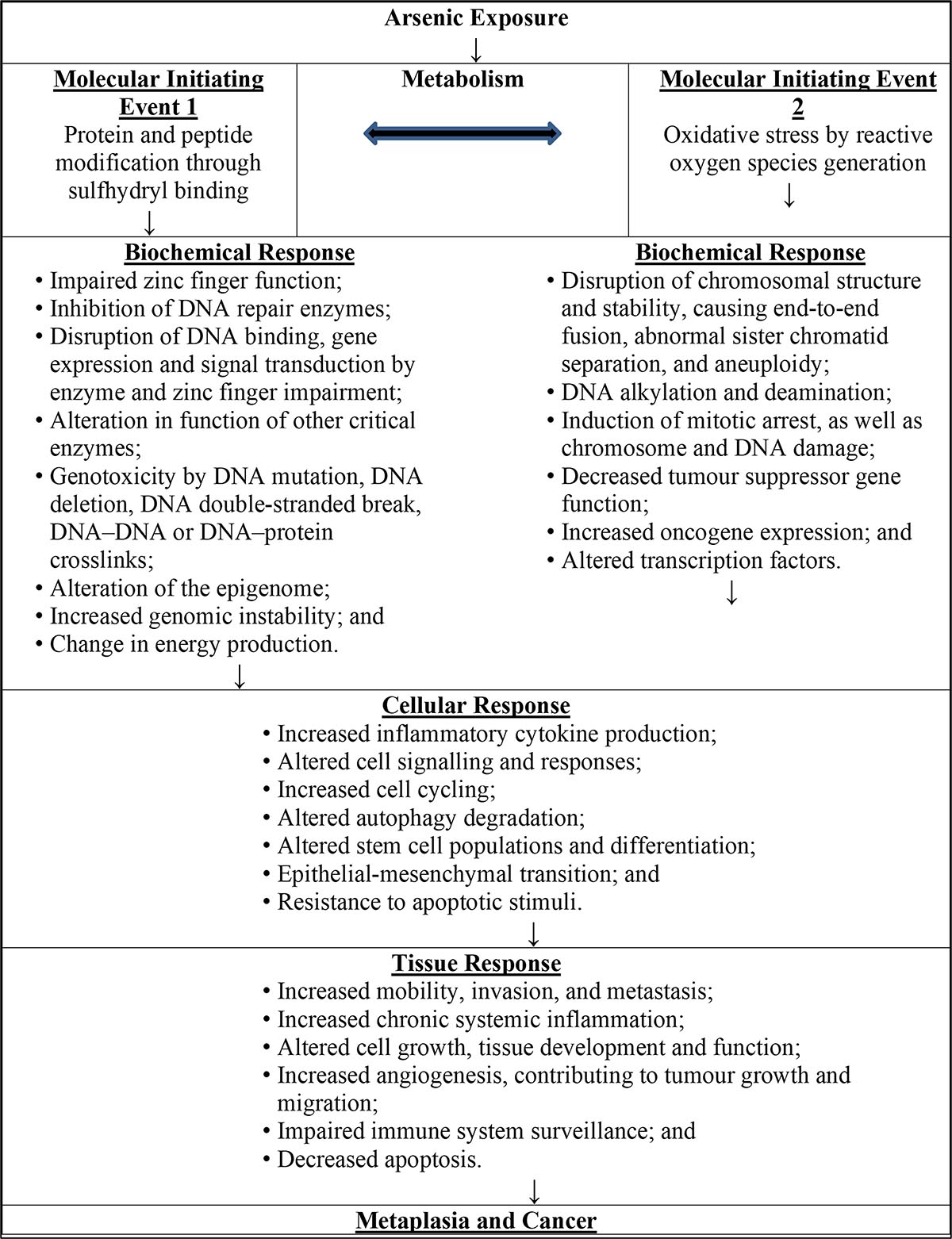
Figure 1: Text description
When exposed to arsenic, arsenic is metabolised which in turn can trigger two different molecular initiating events. Molecular initiating event 1 is protein and peptide modification through sulfhydryl binding. The biochemical response to this molecular initiating event includes: impaired zinc finger function; inhibition of DNA repair enzymes; disruption of DNA binding, gene expression and signal transduction by enzyme and zinc finger impairment; alteration in function of other critical enzymes; genotoxicity by DNA mutation, DNA deletion, DNA double-stranded break, DNA–DNA or DNA–protein crosslinks; alteration of the epigenome; increased genomic instability; and change in energy production. Molecular initiating event 2 is oxidative stress by reactive oxygen species generation. The biochemical response to this molecular initiating event includes: disruption of chromosomal structure and stability, causing end-to-end fusion, abnormal sister chromatid separation, and aneuploidy; DNA alkylation and deamination; induction of mitotic arrest, as well as chromosome and DNA damage; decreased tumour suppressor gene function; increased oncogene expression; and altered transcription factors. The biochemical responses from both molecular initiating events cause the following cellular responses: increased inflammatory cytokine production; altered cell signalling and responses; increased cell cycling; altered autophagy degradation; altered stem cell populations and differentiation; epithelial-mesenchymal transition; and resistance to apoptotic stimuli. These cellular responses cause the following tissue responses: increased mobility, invasion, and metastasis; increased chronic systemic inflammation; altered cell growth, tissue development and function; increased angiogenesis, contributing to tumour growth and migration; impaired immune system surveillance; and decreased apoptosis. These tissue responses can cause metaplasia and cancer.
Although there are data in the literature to support the proposed threshold MOA for cancer, there are significant uncertainties which require consideration when choosing the appropriate dose-response approach. Arsenic-induced cancer is a complex process due to the multiple forms of arsenic (As(III), As(V) and metabolites) which have distinctive potencies and actions with numerous molecular, biochemical and cellular pathway targets. Therefore, predicting cancer incidence based on a single key event is difficult.
The background cancer risk is also an important consideration. For example, in the case of lung cancer, several arsenic-induced key events are expected to be the same as for lung cancer due to other causes, particularly at the cell signalling and transformation levels of organization (RSI, 2023). Arsenic exposure from drinking water can therefore add to the background level of key events already occurring independent of arsenic exposure, with small exposures potentially prompting a cascade of events leading to cancer. Conolly et al. (2005) and Lutz et al. (2005) report that if an unexposed population has a background level of disease or key events, then additional exposure can incrementally add to the background level of response, which will influence the shape of the dose-response curve. Crump et al. (1976) showed that a parameter increasing the rate of a background disease process will show a linear relationship in the presence of additional exposure to that parameter. This supports a low-dose linear (non-threshold) extrapolation approach for dose-response assessment.
Interindividual variability in response to arsenic exposure is another important consideration. Interindividual variability is substantial for arsenic, more so than for other chemical pollutants. As discussed in more detail in section 2.2.2, populations that may be disproportionately impacted can be characterized as those having susceptibility to arsenic effects either due to life stage, reduced methylation capacity (due to gene polymorphisms), dietary factors (such as nutritional deficiencies in folate and selenium), lifestyle factors (such as smoking or co-exposure to other carcinogenic metals) or pregnancy. One or more of these risk modifiers (along with background levels of response) will determine an individual’s threshold dose. At the population level, with numerous risk modifiers to consider, it is likely that variability in response across the population will be substantial and will introduce greater uncertainty into the process of identifying a population threshold of response.
Taking into consideration the complex MOA, the potential additivity of drinking water exposures to ongoing background levels of key events (leading to lung cancer) and the substantial interindividual variability due to the presence of numerous risk modifiers, it is difficult to estimate a population threshold. Furthermore, this threshold would carry a low level of confidence in terms of providing adequate health protection. Taken together, these considerations support a low-dose linear (non-threshold) approach for developing health guidance for arsenic in drinking water.
2.2.5 Selected key studies
The best available epidemiological data show that exposure to low levels of arsenic in drinking water is most strongly associated with lung and bladder cancer. Although there are epidemiological data on non-cancer effects (as discussed in section 2.2.1), the associations and/or dose-response trends at low-dose exposures are generally weak. Therefore, cancer is considered the most appropriate key health endpoint for assessing the health risks from exposure to arsenic in drinking water.
Health Canada commissioned RSI (2022) to conduct a meta-analysis on the best available epidemiological data for the key health endpoints associated with exposure to arsenic in drinking water. Meta-analysis combines evidence from several studies for dose-response modelling to derive points of departure (PODs) (benchmark doses [BMDs] and benchmark dose lower limits [BMDLs]) for lung and bladder cancer (see section 3.0 for details of the analysis). As shown in Table 6, the analysis revealed lung cancer to be a more sensitive health endpoint than bladder cancer as indicated by the lower BMD/BMDL values.
The five key lung cancer studies that provided sufficient information for conducting a meta-analysis are listed in Table 7. These include the studies by Smith et al. (2009) and Chen et al. (2010b), as described in section 2.1.1, as well as three additional supportive studies with adequate data for meta-analysis (Mostafa et al., 2008; Dauphine et al., 2013; Steinmaus et al., 2013).
| Endpoint | Model and data (# of studies/ # of data points) | BMD based on 1% excess risk (µg/L) | BMD based on 5% excess risk (µg/L) | BMD based on 10% excess risk (µg/L) | |||
|---|---|---|---|---|---|---|---|
| BMD01 | BMDL01 | BMD05 | BMDL05 | BMD10 | BMDL10 | ||
| Bladder cancer | Log-linear; 8/31 | 122.5 | 33.5 | 417.0 | 113.7 | 623.1 | 169.6 |
| Lung cancer | Log-linear; 5/15 | 60.4 | 14.4 | 241.9 | 57.5 | 396.1 | 93.9 |
| BMD: benchmark dose; BMDL: benchmark dose lower limit | |||||||
| Study | Study design | Location | Sample size | Dose metric | Number of study groups | Reference dose range less than 10 μg/L? Dose groups | Risk (95% CI) |
|---|---|---|---|---|---|---|---|
Mostafa et al. (2008) |
Case-control (males only) |
Bangladesh |
516 cases (non-smokers), 2 239 cases (smokers), 438 controls (non-smokers), 735 (smokers) |
Tube-well water concentration (µg/L) |
4 |
Yes Less than 10, 11 to less than or equal to 50, 51 to less than or equal to 100, 101 to less than or equal to 400 µg/L |
Smokers ORs: 1.00, 1.25 (0.96 to 1.62), 1.37 (0.92 to 2.03), 1.65 (1.25 to 2.18); Non-smokers ORs: 1.00, 0.90 (0.62 to 1.33), 1.10 (0.62 to 1.96), 0.94 (0.62 to 1.41) |
Smith et al. (2009) |
Case-control |
Chile |
151 cases and 419 controls |
Drinking water concentration (µg/L) |
6 |
Yes 0 to 9, 10 to 59, 60 to 199, 200 to 399 µg/L, 400 to 699 and 700 to 999 |
ORs: 1.00, 0.7 (0.3 to 1.7), 3.4 (1.8 to 6.5), 4.7 (2.0 to 11.0), 5.7 (1.9 to 6.9) and 7.1 (3.4 to 14.8) |
Chen et al. (2010b) |
Prospective cohort |
Northeastern Taiwan |
6 888 |
Well water concentration (µg/L) |
5 |
Yes less than 10 µg/L, 10 to 49.99 µg/L, 50 to 99.99 µg/L, 100 to 299.99 µg/L, equal to or greater than 300 µg/L |
RRsTable 7 Footnote a: 1.00, 1.10 (0.74 to 1.63), 0.99 (0.59 to 1.68), 1.54 (0.97 to 2.46) and 2.25 (1.43 to 3.55) RRsTable 7 Footnote b: 1.00, 1.22 (0.64 to 2.32), 1.32 (0.64 to 2.74) |
Dauphine et al. (2013) |
Case-control |
United States (California/ Nevada) |
196 cases and 359 controls |
Average drinking water concentration (µg/L) |
3 |
Yes Less than 10, 11 to 84, equal to or greater than 85 µg/L |
ORs for highest 5-year average, 40-year lag: 1.0, 0.84 (0.40 to 1.79), 1.39 (0.55 to 3.53) |
Steinmaus et al. (2013) |
Case-control |
Chile |
306 cases and 640 controls |
Average drinking water concentration (µg/L) |
4 |
No Lifetime average concentrations before 1971: less than 11, 11 to 90, 91 to 335, greater than 335 µg/L |
ORs: 1.00, 1.27 (0.81 to 1.98), 2.00 (1.24 to 3.24), 4.32 (2.60 to 7.17) |
CI: confidence interval; OR: odds ratio; RR relative risk
|
|||||||
3.0 Derivation of the health-based value (HBV)
The weight of evidence continues to support cancer as the key health endpoint showing the strongest association with exposure to low concentrations of arsenic in drinking water. Furthermore, following the evaluation of the best available epidemiological evidence on cancer effects, lung cancer is considered the most sensitive health endpoint (see section 2.2.4) for assessing the health risks from exposure to arsenic in drinking water.
Although there are some data available to support a threshold MOA for lung cancer, several significant uncertainties remain with respect to how low-level arsenic exposure leads to cancer, as discussed in section 2.2.3. This calls into question the appropriateness of a threshold approach. This includes uncertainty surrounding which arsenic event(s)/pathway(s)/form(s) play a key role in causing cancer; the potential for exposure to arsenic in drinking water to add to ongoing background levels of key events (leading to lung cancer) occurring from exposure either to arsenic from other sources or exposure to other lung cancer-causing substances; and substantial interindividual variability across the Canadian population (see section 2.2.2) due to numerous risk modifiers that can alter an individual’s response to arsenic exposure. Considering these significant uncertainties, a low-dose linear approach for assessing the risk of lung cancer from exposure to arsenic in drinking water is considered most appropriate.
To derive a POD for lung cancer, RSI (2022) conducted a meta-analysis combining the dose-response results from key lung cancer studies (see section 2.2.5) for BMD modelling. Meta-analysis is a statistical procedure that involves combining data from multiple studies in order to overcome individual study limitations (such as limited sample size, wide confidence intervals and variations in study design). In the present context, the ultimate goal was to reduce uncertainty associated with the derived BMDs/BMDLs. Although benchmark responses of 1%, 5% and 10% were modelled, the 1% response data were chosen due to the severity of the health endpoint. The analysis outputs are presented in Table 8.
A pooled analysis of relative risks from the five studies identified in section 2.2.4 was performed for arsenic exposures at or below 250 µg/L, in order to reduce the influence of responses to very high exposure levels, which are not representative of typical drinking water exposures in Canada. Log-linear parametric models were used to describe the shape of the dose-response curve within the observable response range. A two-stage log-linear model was used to derive slope parameter estimates for each study, then weighted averages were used to derive a slope parameter estimate for the meta-analysis. It was assumed that a random-effects model was more appropriate than a fixed-effects model due to heterogeneity between studies. Heterogeneity (I2; Table 8) is an indicator of differences in study parameters across studies, including study design, participant characteristics and average exposure levels. In the meta-analysis of all five studies, although the p-value of 0.418 for the “goodness of fit” test shows an acceptable fit (a p-value greater than 0.1 indicates a suitable fit), the heterogeneity statistic of 80.6% (CI: 54.7% to 91.7%) indicates substantial differences among the studies. Deeks et al. (2021) provides guidance on interpreting heterogeneity as follows: not important (0% to 40%), moderate (30% to 60%), substantial (50% to 90%) and considerable (75% to 100%). When high degrees of heterogeneity exist, caution should be exercised when interpreting BMD modelling results. In the Smith et al. (2009) study, the highest exposure group (60 to 199 ug/L) may be an influential group in the overall meta-analysis due to its large OR compared to that of the highest exposure groups in the other studies. When the meta-analysis is performed with the Smith et al. (2009) study data removed, the heterogeneity statistic is reduced to 42.1% (CI: 0%, 80.6%). Also, the resulting excess 1% risk BMD01 and BMDL01 estimates increase to 174.8 and 32.9 µg/L, respectively, compared to the BMD01 and BMDL01 values of 60.4 and 14.4 µg/L, respectively, when the Smith et al. (2009) study data are included. Although excluding the data from a given study (for instance, the Smith et al., 2009 study) may reduce heterogeneity, this alone should not be viewed as sufficient justification for removing a study or its observations from the analysis. Therefore, it is important that the Smith et al. (2009) study data be included in the overall BMD analysis for lung cancer.
The meta-analysis for lung cancer was performed by fitting dose-response models to relative risk values from the key lung cancer studies in order to determine excess risk-based BMDs. The BMD analyses were carried out using a log-linear model from the dosresmeta R package for conducting multivariate dose-response meta-analysis (software version 4.1.1), with the choice of model based on the “goodness of fit” test. Drinking water arsenic concentrations were standardized to arsenic exposure by applying an adult daily water consumption of 1.53 L/day and a body weight of 74 kg for the population in Canada (Health Canada, 2022b). Modelling required the incorporation of a Canadian background average arsenic level in drinking water and a background lung cancer risk level. The average person in Canada was assumed to be exposed to inorganic arsenic in drinking water at 2.25 µg/L, which represents the midpoint value of the average groundwater concentrations reported in several Canadian provinces (Health Canada, 2006a). The estimated risk for lung cancer associated with current background exposure levels in Canada is 6.7% (Canadian Cancer Statistics Advisory Committee, 2021).
Using a total of 15 data points from the 5 key studies identified in section 2.2.4, the BMD01 and BMDL01 values representing a 1% excess risk of lung cancer above the Canadian background level were estimated to be 60.4 and 14.4 µg/L, respectively, as shown in Table 8.
| Study (# of studies)Table 8 Footnote a |
p-value (goodness of fit)Table 8 Footnote b | Excess Risk (1%) | ||
|---|---|---|---|---|
| BMD01 (µg/L) | BMDL01 (µg/L) | BMDU01 (µg/L) | ||
Meta-analysis (5) |
0.418 |
60.4 |
14.4 |
ND |
| Meta-analysis (4) excluding Smith et al. (2009) | 0.598 | 174.8 | 32.9 | ND |
| Dauphine et al. (2013) | 0.401 | ND | 61.1 | ND |
| Chen et al. (2010b) | 0.599 | 5153.6 | 49.6 | ND |
| Mostafa et al. (2008) | 0.408 | 288.7 | 36.4 | ND |
| Smith et al. (2009) | 0.110 | 15.5 | 11.0 | 26.3 |
| Steinmaus et al. (2013) | 0.357 | 38.2 | 21.1 | 217.4 |
ND: not determined; the benchmark dose upper limit (BMDU01) cannot be determined since its derivation is based on the lower confidence limit for the dose-response slope, which is negative. However, the “best” estimate for a POD, based on available epidemiologic data, is the BMDL01, which accounts for uncertainty in the POD estimation. The BMDL01 can be determined since it is derived based on the upper confidence limit for the dose-response slope which is positive.
|
||||
To apply a low-dose linear extrapolation approach using the BMDL01 of 14.4 µg/L, the slope of the dose-response curve is determined as follows:
Slope = excess risk level / POD
= 0.01 / 14.4 µg/L
≈ 0.0007 (µg/L)-1 (1)
where:
- the excess risk level represents a 1% excess risk of lung cancer above the Canadian background level; and
- the POD is the point of departure at 1% excess risk above the Canadian background level of 14.4 µg/L.
Using the slope of the dose-response curve, a risk-specific dose can be determined as follows:
Risk-specific dose = risk level / slope
In the context of drinking water guidelines, Health Canada defines “essentially negligible” as a range from one new cancer above background per 1 million people to one new cancer above background per 100 000 people (10-6 to 10-5) over a lifetime. Table 9 shows the estimated excess lifetime risk of lung cancer (above the Canadian background level) associated with various concentrations of arsenic in drinking water.
| Level of arsenic in drinking water (µg/L) | Estimated excess lifetime risk of lung cancer above the Canadian background level |
|---|---|
| ≈ 0.0014 | 1 × 10⁻⁶ |
| ≈ 0.014 | 1 × 10⁻⁵ |
| ≈ 0.14 | 1 × 10⁻⁴ |
| Proposed MAC = 5 ug/L | 3.5 × 10⁻³ |
| Current MAC = 10 µg/L | 7 × 10⁻³ |
The level of arsenic in drinking water that represents an “essentially negligible” risk of lung cancer ranges from 0.0000014 to 0.000014 mg/L (0.0014 to 0.014 µg/L). Since people in Canada can be exposed to arsenic through multiple sources (such as food, drinking water, air and soil; see section 1.3), the health-based value (HBV) for drinking water is set to 0.0000014 mg/L (0.0014 µg/L), which is near the lower level of the range.
4.0 Analytical methods for detecting arsenic
4.1 Standardized methods
Standardized analytical methods available for the analysis of total arsenic in drinking water and their respective method detection limits (MDLs) are summarized in Table 10. MDLs are dependent on the sample matrix, instrumentation and selected operating conditions, and will vary between individual laboratories. These methods are subject to a variety of interferences, which are outlined in the respective references. The total arsenic concentration is determined using these methods but the different arsenic species are not differentiated.
Accredited laboratories in Canada were contacted to determine the MDLs; these laboratories’ method reporting limits for total arsenic analysis were between 0.5 and 1 μg/L for methods based on inductively coupled plasma–mass spectrometry (ICP-MS) (AGAT Laboratories, 2019a,b,c; Paracel Laboratories Ltd., 2019). Drinking water treatment systems should discuss sampling requirements with the accredited laboratory conducting the analysis to ensure that quality control procedures are followed. Also, the method reporting limits need to be low enough to ensure accurate monitoring at concentrations below the proposed MAC.
| Method (Reference) |
Methodology | MDL (µg/L) |
Comments |
|---|---|---|---|
EPA 200.5 Rev. 4.2 (U.S. EPA, 2003a) |
Axially viewed ICP-AES |
0.1 |
Matrix interferences: Ca, Mg and Na > 125 mg/L and Si > 250 mg/L |
EPA 200.7 Rev. 4.4 (U.S. EPA, 1994a) |
ICP-AES |
1.0 |
Matrix interferences: TDS > 0.2% (w/v) |
EPA 200.8 Rev. 5.4 (U.S. EPA, 1994b) |
ICP-MS |
0.03–0.5 |
Matrix interferences: TDS > 0.2% (w/v) |
EPA 200.9 Rev. 2.2 (U.S. EPA, 1994c) |
Stabilized temperature graphite furnace atomic absorption spectrometry |
0.05 |
The HCl present from digestion procedure can influence the sensitivity. |
SM 3113 (APHA et al., 2023) |
Electrothermal atomic absorption spectrometry |
0.5 |
Matrix modification can be useful in minimizing interferences and increasing sensitivity. Optimum concentration: 5–100 μg/L |
SM 3125 (APHA et al., 2023) |
ICP-MS |
0.025 (IDL) |
Samples should not contain > 0.5% dissolved solids. |
D5673-16 (ASTM, 2016) |
ICP-MS |
0.9 (IDL) |
None |
| ICP-AES: Inductively coupled plasma–atomic emission spectrometry; ICP-MS: Inductively coupled plasma–mass spectrometry; IDL: instrument detection level; MDL: method detection limit; SM: Standard Method; TDS: total dissolved solids | |||
4.2 Sample preparation
Total arsenic includes both the dissolved and particulate fractions of arsenic in a water sample. Methods used for total recoverable arsenic are used to analyze total arsenic, which is compared to the proposed MAC.
Sample processing considerations for the analysis of arsenic in drinking water (for example, sample preservation, storage, digestion) can be found in the references listed in Table 10. Accurate quantification of dissolved, particulate and total arsenic is dependent on proper sample preservation and processing steps. Standard Method (SM) 3030B and SM 3030D provide guidance on filtration, preservation (acidification) and digestion procedures for the determination of dissolved or particulate metals (APHA et al., 2023). To determine dissolved arsenic concentrations, samples should be filtered at the time of collection (not at the laboratory). The filtrate should be acidified to a pH of less than 2 with concentrated nitric acid.
Currently, EPA methods 200.8 and SM 3113 do not require hot acid digestion for total recoverable metals, unless turbidity of the sample is greater than 1 nephelometric turbidity unit. However, studies conducted on other metals (for example, lead, chromium) have found that this does not accurately quantify the total metal concentration in a drinking water sample (Triantafyllidou et al., 2007, 2013; Deshommes et al., 2010; Haas et al., 2013; Clark et al., 2014). When particulate arsenic is present, this approach may underestimate total arsenic in drinking water. Hot acid digestion is described in EPA method 200.8 Rev. 5.4 (U.S. EPA, 1994b). Microwave-assisted digestion, outlined in SM 3030 K (APHA et al., 2023), can also be used for analysis of total recoverable metals in the case of methods that are based on ICP-MS.
4.3 Online analyzers and portable field kits
Commercial online analyzers are available for quantifying dissolved or soluble arsenic. Some online analyzers have an internal digestion unit that can measure both dissolved and total arsenic. Depending on the analyzer, arsenic may be determined through voltammetry or spectrophotometry. Online analyzers have various ranges depending on the unit and have detection limits of 1 μg/L or less.
A field arsenic speciation method is presented in Edwards et al. (1998). This method uses an anion exchange resin column to separate the soluble arsenic species. A filtration step using a 0.45 μm filter is used to separate the soluble and insoluble forms of arsenic (Sorg et al., 2014). This method allows for determination of total arsenic, particulate arsenic, soluble arsenic, soluble As(III) and soluble As(V).
Portable test kits are also available that are based on colorimetric methods and cover various ranges. A review of various portable test kits is presented in He et al. (2023) and includes the ranges, performance and references. The authors of this review indicate that on-site test kits do not guarantee the same performance as analytical methods in the laboratory. They recommend taking duplicate samples, blank samples and spiked samples, and comparing against standardized methods.
To accurately measure arsenic using these units, water treatment systems should develop a quality assurance and quality control (QA/QC) program such as those outlined in SM 3020 (APHA et al., 2023). In addition, periodic verification of results using an accredited laboratory is recommended. Water treatment systems should check with the responsible drinking water authority to determine whether results from these analyzers can be used for compliance reporting.
5.0 Treatment considerations
Treatment technologies that may be used to reduce the concentration of arsenic at the municipal scale for drinking water are co-precipitation/adsorption, adsorption, membrane filtration, ion exchange and enhanced lime softening. A combination of these treatment technologies could also be used to achieve lower arsenic concentrations. The selection of treatment technology depends on several factors, including source water chemistry, existing treatment processes, operational conditions and residual handling concerns. Pilot-scale testing is critical to ensure the source water can be successfully treated and to optimize operating conditions. Bench-scale testing can be used to determine operational parameters for optimal arsenic removal performance for a full-scale system.
At the residential scale, certified treatment devices relying on RO, adsorption or distillation are expected to be effective for removal of arsenic.
5.1 Arsenic chemistry
Inorganic forms of arsenic are more prevalent in water. The species present depend on oxidation-reduction conditions and pH (Fields et al., 2000a; U.S. EPA, 2003b; Sorg et al., 2014). Arsenic is generally present in the reduced form, that is As(III), in groundwater under anoxic conditions and lower redox potentials. In surface waters under aerobic conditions, the oxidized form, that is As(V), is usually present (Fields et al., 2000a; U.S. EPA, 2003b; Katsoyiannis et al., 2007; Ahmad et al., 2017). In the environment, the oxidation or reduction of arsenic is a slow process and a proportion of each species is generally present (Edwards, 1994).
The U.S. EPA’s arsenic treatment research program collected monthly arsenic speciation data in 65 wells for up to 3 years (Sorg et al., 2014). Although, as previously stated, groundwater generally contains arsenic in the form of As(III), this speciation study showed that it is not uncommon for groundwater to also contain As(V). The data from these groundwater sources showed that 31 of the 65 wells had mostly As(V), 29 had predominantly As(III) and 5 had a mixture. The monthly tests from these wells showed that there were no significant changes in the speciation over time.
For arsenic removal, the species (As(III) versus As(V)) is an important factor. Since As(III) exists mainly as the neutral species H3AsO3 at a pH below 9, it is not easily removed by most treatment technologies (U.S. EPA, 2003b; Ahmad et al., 2017). As As(V) exists mainly as the single-charged species H2AsO4- or the double-charged species HAsO42-, at pH values between 6 and 9, it can be effectively removed by the available treatment methods (U.S. EPA, 2003b; Ahmad et al., 2017). As such, oxidation of As(III) to As(V) is critical in the treatment process in order to achieve effective removals (Ahmad et al., 2017).
The amount of soluble versus particulate arsenic is an important factor in determining appropriate treatment. The prevalence of particulate arsenic in some source waters may indicate that filtration alone would reduce arsenic sufficiently (Edwards et al., 1998; Chen et al., 1999). In one study, 428 water supplies were sampled and greater than 96% particulate arsenic was found in one groundwater sample, greater than 50% particulate arsenic in 30% of groundwater samples, and between 23% and 54% particulate arsenic in surface water samples (Chen et al., 1999).
5.2 Municipal-scale treatment
The selection of an appropriate treatment process for arsenic removal for a specific water supply is complex and depends on many factors such as water quality (including arsenic concentration, arsenic species, soluble iron concentration and pH), existing treatment processes, system/operation reliability and simplicity, and residual production and disposal. The form of arsenic (soluble or particulate) and the proportion of each species present also impact treatment choice.
Arsenic readily adsorbs to soluble iron. Iron plays a significant role in arsenic removal whether present in the source water or added to the treatment process. For this reason, iron is a critical factor in the selection of an appropriate treatment, including iron removal processes (Wang et al., 2004). Iron removal processes include chemical oxidation/filtration, biological oxidation, and manganese greensand filtration (U.S. EPA, 2003b; Hoffman et al., 2006). Sorg (2002) developed a tool that defines zones based on the ratio of soluble iron to arsenic concentration. The tool guides the selection of potential treatment technologies for arsenic removal in relation to these defined zones (see Figure 2). For water falling into Zone A, the soluble iron to soluble arsenic concentrations would favour the selection and optimization of an iron removal process (for example, a 20:1 soluble iron to arsenic ratio is the minimum required for chemical oxidation/filtration; see section 5.2.2). For Zone B water, there is insufficient soluble iron, and a modified iron removal process should be considered. For Zone C, low soluble iron levels indicate that technologies to consider for arsenic removal include adsorption, ion exchange, iron coagulation/filtration, modified iron removal and membrane processes.
Figure 2. Tool to assess treatment technologies for arsenic removal (adapted from Sorg, 2002)
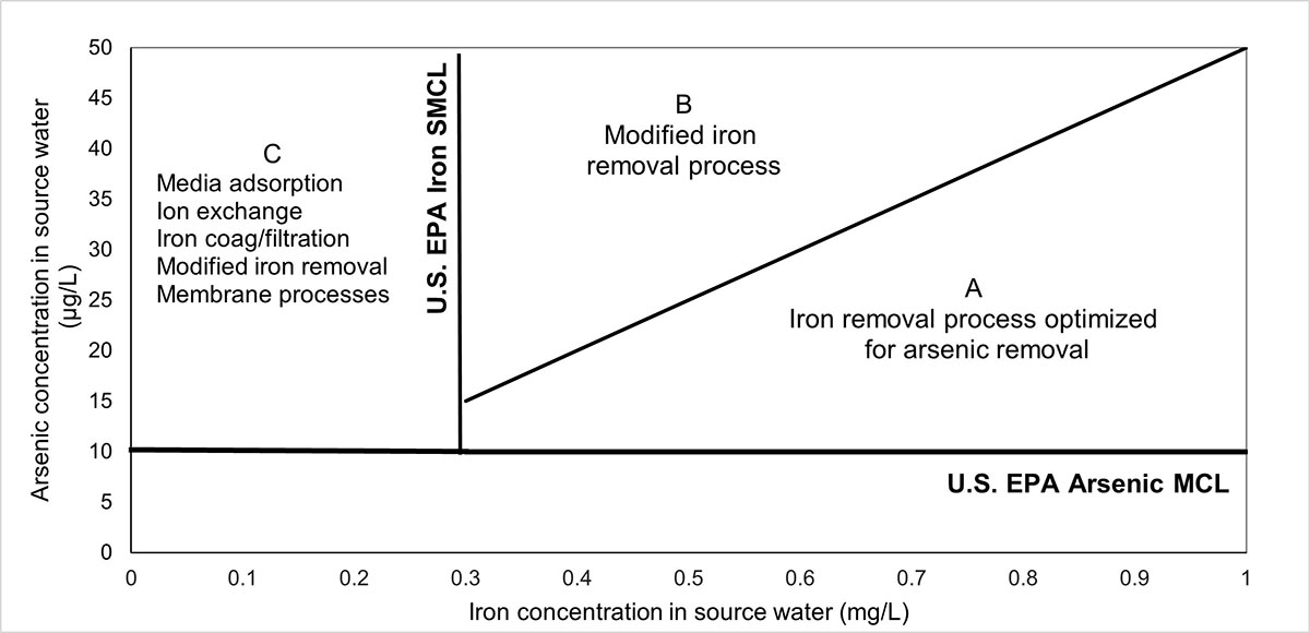
MCL: Maximum contaminant level; SMCL: secondary maximum contaminant level
Figure 2: Text description
This figure has zones to aid in determining appropriate treatment for a source water based on iron and arsenic source water concentrations. For higher iron concentrations (greater than 0.3 mg/L) and lower arsenic concentrations (below 0.015 mg/L), Zone A indicates that an iron removal process may be chosen. For iron and arsenic concentrations above these concentrations, Zone B indicates that a modified iron removal process may be preferred. For lower iron concentrations (less than 0.3 mg/L), Zone C indicates that an alternate treatment technology should be chosen.
The presence of competing ions may have an impact on the effectiveness of different treatment technologies. Phosphates, sulphate, natural organic matter (NOM), silicates, fluoride, carbonates, vanadium, selenium and trace heavy metals have the potential to negatively impact arsenic removal depending on the technology being used (Fields et al., 2000a,b; Korngold et al., 2001; Rubel, 2003a,b; U.S. EPA, 2003b; Sancha, 2006; Guan et al., 2009a,b; Pallier et al., 2010; Clifford et al., 2011; Möller et al., 2011; Mondal et al., 2013; Sorlini et al., 2014; Cortina, 2016; Hering et al., 2017; Mohanty, 2017; Sorg et al., 2017a; van Genuchten and Ahmad, 2020). Owing to its similar chemistry, phosphate competes strongly with arsenic in various treatment technologies. The presence of calcium was found to improve arsenic removal for conventional treatment and for chemical oxidation/filtration (van Genuchten and Ahmad, 2020; Guan et al., 2009b).
Health Canada strongly recommends that any chemicals and components used in treatment systems be certified to NSF/ANSI/CAN Standard 60: Drinking Water Treatment Chemicals–Health Effects (NSF International, 2024a), NSF/ANSI/CAN Standard 61: Drinking Water System Components–Health Effects (NSF International, 2023a). These standards ensure that materials meet health-based requirements and are safe for use in potable water applications.
The following subsections present full- and pilot-scale studies. These include studies from a U.S. EPA full-scale demonstration program that evaluated various treatment technologies at small and semi-public systems. This program generally monitored the systems over several years. In some cases, the systems were modified during the study in an attempt to improve arsenic removal (U.S. EPA, 2023).
5.2.1 Pre-oxidation
Most, and potentially all, treatment technologies remove As(V) better than As(III) although they may require pH adjustment for optimization. When significant As(III) is present, pre-oxidation will improve arsenic removal. Arsenic can be rapidly oxidized under many conditions using chlorine, permanganate, ozone, and manganese dioxide-based solid-oxidizing media (Ghurye and Clifford, 2001, 2004; Katsoyiannis et al., 2004; Dodd et al., 2006; Sorlini and Gialdini, 2010; Clifford et al., 2011). However, oxygen, aeration, chlorine dioxide, chloramine and ultraviolet irradiation are not effective in oxidizing arsenic (Bissen and Frimmel, 2003; U.S. EPA, 2003b; Ghurye and Clifford, 2004; Hoffman et al., 2006; Sorlini and Gialdini, 2010; Mohanty, 2017). If chlorine is added in the presence of ammonia, chloramines will form and negatively impact the oxidation of As(III) (Chen et al., 2018). The presence of NOM in source water can also impede the oxidation of As(III) when permanganate (Chen et al., 2018) and ozone are being used (Ghurye and Clifford, 2001). The appropriate permanganate dosage can be determined through a jar test, as outlined in the study conducted by Chen et al. (2018).
Biological oxidation of As(III) by iron- or manganese-oxidizing bacteria can also occur (Gude et al., 2018a; Crognale et al., 2019). There are also arsenic-oxidizing bacteria that can grow and survive within filters (Lytle et al., 2007). When pre-oxidation is achieved using arsenic-oxidizing bacteria, pre-aeration is needed to ensure the growth and development of the bacteria (Lytle et al., 2007; Gude et al., 2018a,b; Crognale et al., 2019). Microbial development under these conditions has been shown to take between 10 days and a month to establish (Zouboulis and Katsoyiannis, 2005; Lytle et al., 2007). Running aerated water through new filter media promotes rapid bacteria growth, and seeding with old filter media was found to be unnecessary (Lytle et al., 2007).
Choice of oxidant and point of addition are important design considerations and will depend on raw water quality (Hoffman et al., 2006). The pre-oxidation strategy should include an assessment to determine if any disinfection by-products (DBPs) are formed and to confirm that no other compliance issues occur. Bench- and pilot-scale studies can help optimize an oxidation strategy.
5.2.2 Co-precipitation/adsorption
Coagulation/filtration and iron removal processes remove arsenic through a combination of co-precipitation and adsorption. In waters with large amounts of soluble ferrous (Fe(II)), iron removal processes can be used to simultaneously remove arsenic (Sorg, 2002; U.S. EPA, 2005). When the amount of iron is insufficient, a coagulant is added in a coagulant/filtration process. When oxidation occurs, iron and arsenic are co-precipitated and the arsenic adsorbs to newly formed ferric oxide (Fe(III)) (Sorg, 2002; Katsoyiannis and Zouboulis, 2004; Hoffman et al., 2006; Chen et al., 2018).
As pre-formed iron particles have less capacity to remove As(V) than iron particles that are formed in the presence of As(V), oxidation of iron and arsenic should occur at the same time to achieve optimal arsenic removal (Edwards, 1994; Roberts et al., 2004; Tresintsi et al., 2013). These processes improve with increasing natural iron in the water and increasing particle surface area (Lytle et al., 2005; Hoffman et al., 2006; Thirunavukkarasu et al., 2014).
Coagulation/filtration
Coagulation/filtration is the most frequently used conventional method to treat arsenic in water and is suitable for large-capacity drinking water treatment systems (Chen et al., 2002; U.S. EPA, 2005; Cortina, 2016). Arsenic-laden flocs are formed through the addition of a coagulant and then removed through sedimentation and filtration (U.S. EPA, 2005; Sancha, 2006; Mondal et al., 2013; Cortina, 2016). Effective removal is a function of arsenic species and initial concentration, coagulant type and dose, mixing intensity, pH and water composition (Sancha, 2006; Hering et al., 2017). The coagulants commonly used in arsenic removal by coagulation/filtration are aluminum sulphate (alum), ferric chloride, ferrous sulphate and cationic polymers (Fields et al., 2000b; Han et al., 2002; Sancha, 2006; Cortina, 2016). An optimized system can achieve greater than 90% arsenic removal (U.S. EPA, 2005). A selection of full-scale studies are presented in Table 11.
Greater removal of As(V) than As(III) was observed at all pH values and coagulants (U.S. EPA, 2005; Lakshmanan et al., 2008; Sun et al., 2013; Sorlini and Gialdini, 2014; Cortina, 2016). The presence of ammonia may have resulted in chloramine formation and thus incomplete oxidation of As(III) to As(V) (Valigore et al., 2008a).
Ferric-based coagulants were shown to have better arsenic removal than aluminum-based coagulants (U.S. EPA, 2000; Odell, 2010). Typical doses of ferric-based coagulants shown to be effective are 5 to 30 mg/L, with better removals at a pH less than 8 (U.S. EPA, 2003b; Lakshmanan et al., 2008; Odell, 2010; Cortina, 2016). Alum coagulation (typical dose of 10 to 50 mg/L, at pH 6 to 7) is less effective than ferric-based coagulation for As(V) and does not remove As(III) (Lakshmanan et al., 2008; Cortina, 2016).
As(V) removal depends on coagulation dose and pH, along with the zeta potential of the colloidal suspension (Edwards, 1994; Pallier et al., 2010; Hu et al., 2012; Pramanik et al., 2016). A lower pH increases positively charged adsorption sites and decreases the concentration of the competing OH- ions (Ghurye et al., 2004; Sancha, 2006; Pramanik et al., 2016). Lowering the pH below 7 can lead to increased removal and require less coagulant (Sancha, 2006; Lakshmanan et al., 2008; Cortina, 2016; Hering et al., 2017). As(III) removal depends on coagulant dose and, to a smaller extent, on pH (Edwards, 1994; Pallier et al., 2010). However, since As(V) is more readily removed than As(III), pre-oxidation of all As(III) to As(V) prior to conventional coagulation/filtration is the preferred approach. A study by Sorlini et al. (2014) evaluating 8 full-scale treatment plants showed that the highest rate of removal was achieved when either a double stage of iron addition or post-iron adsorption was implemented.
With the required coagulant doses for arsenic removal, significant amounts of arsenic-laden sludge may be produced. This may lead to challenges in disposing of the contaminated sludge. Sludge production is a significant drawback for conventional coagulation/filtration utilization in arsenic removal from drinking water.
| Influent arsenic (μg/L) |
Treated water arsenic (μg/L) |
Other source water parameters | Coagulant | Operational parameters | Reference |
|---|---|---|---|---|---|
| Municipal-scale | |||||
7.5 [As(III) = 0.7] |
3.5 |
Groundwater and surface water runoff through aqueduct pH = 8.0 Soluble Fe < 30 μg/L TOC = 2.4 mg/L (as C) |
FeCl3 = 1 to 2 mg/L (as Fe) Cationic polymer = 1 to 5 mg/L |
Pre-ozonation (1.5 mg/L) Flocculation contact time = 8.5 min Flow rate = 420 mgd Filter media: Anthracite coal Post-chlorination (2 mg/L residual) |
Fields et al. (2000b) |
19.1 [As(III) = 0.6] |
4.0 |
Surface water pH = 8.4 Soluble Fe < 30 μg/L TOC = 3.7 mg/L (as C) |
Alum = 25 to 30 mg/L Cationic polymer = 0.75 mg/L |
Pre-chlorination Flow rate = 6 to 8 mgd in winter and 30 to 35 mgd in summer Filter media: anthracite/sand |
|
20 [As(III) = 14] |
4 |
Groundwater pH = 7.9 Fe = 165 μg/L Phosphate = 550 μg/L NH3 = 1.2 mg/L |
FeClSO4 = 2.3 mg/L (as Fe) |
Biological oxidation Filter media: Anthracite/sand Backwash every 3 days |
Katsoyiannis et al. (2008) |
11.9 ± 1.0 [As(III) = 11.7 ± 1.0] |
< 1 (Prior to coagulant being used As ~ 6.3 μg/L) |
Groundwater pH = 7.6 ± 0.1 Fe = 1400 ± 70 μg/L [as Fe(II)] NH3 = 0.55 ± 0.1 mg/L TOC = 2.4 ± 0.2 mg/L (as C) |
FeCl3 = 1.8 mg/L [as Fe(III)] |
Pre-oxidation with KMnO4 (1.2 mg/L MnO4-) Flow rate = 10 Mm3/yr Filter: Rapid sand |
Ahmad et al. (2018) |
34.4 [As(III) = 29.1] |
8.3 |
Groundwater pH = 8.3 Soluble Fe = 26.1 μg/L SiO2 = 9.5 mg/L (as SiO2) P = 44.7 μg/L (as P) |
FeCl3 = 2.2 mg/L (as Fe) |
Pre-chlorination Contact time = 4.3 min Flow rate = 263 gpm for 6.5 hr/day Filtration rate = 7.0 gpm/ft2 Filter media: Ceramic |
Chen et al. (2010c) (U.S. EPA demonstration program) |
| Other systems | |||||
29.0 [As(III) = 26.2] |
2.7 |
Groundwater pH = 7.8 Soluble Fe = 146 μg/L SiO2 = 14.1 mg/L (as SiO2) |
FeCl3 = 1.8 mg/L (as Fe) |
Seasonal resort Pre-chlorination Contact time = 23 min Flow rate = 49 to 53 gpm Filtration rate = 4.0 gpm/ft2 Filter media: Anthracite |
Chen et al. (2011a) (U.S. EPA demonstration program) |
| Fe: iron; FeCl3: ferric chloride; FeClSO4: iron chloride sulphate; Fe(II): ferrous; Fe(III): ferric oxide; gpm: gallons per minute; KMnO4: potassium permanganate; mgd: million gallons per day; Mm3: cubic megameter; MnO4-: permanganate; NH3: ammonia; P: phosphorus; SiO2: silica; TOC: total organic carbon | |||||
Chemical oxidation/filtration
For chemical oxidation/filtration to be successful, the soluble iron to arsenic ratio in the source water must be at least 20:1 (Sorg, 2002; U.S. EPA, 2003b, 2005). This process involves strong oxidant addition, sufficient contact time and filtration and can be used over a pH range of 5.5 to 8.5 (U.S. EPA, 2003b; Ghurye and Clifford, 2004; Hoffman et al., 2006).
Since chlorine, potassium permanganate and ozone achieve oxidation rapidly, contact time is not a critical factor for these oxidants. However, extended contact time may allow for more particle development and better removal through subsequent filtration (Hoffman et al., 2006). Jar tests are recommended to determine the optimum oxidant dose (Hoffman et al., 2006).
The point at which the oxidant is added is important as iron particles formed in the presence of As(V) have better removal capacity (Lytle et al., 2005; Hoffman et al., 2006; Tresintsi et al., 2013). A bench-scale study evaluated co-oxidation of As(III) (50 μg/L), Fe(II) (5 mg/L) and manganese oxide (Mn(II)) (0.5 mg/L), and showed that chlorine and potassium permanganate are capable of reducing the arsenic level to below 10 μg/L, with potassium permanganate achieving the greatest reduction (van Genuchten and Ahmad, 2020). The presence of NOM in source water can also impede the oxidation of As(III) by permanganate (Chen et al., 2018). Ozone is also effective (Ghurye and Clifford, 2004). Oxidation can be impeded by NOM and other contaminants (Ghurye and Clifford, 2004; Chen et al., 2018). Although aeration can effectively oxidize Fe(II), it is ineffective in oxidizing arsenic (van Genuchten and Ahmad, 2020).
Oxidation/filtration continuously provides new sites for arsenic adsorption, hence there is no need for filter regeneration (Pokhrel and Viraraghavan, 2009). Formation of DBPs must be considered when using chemical oxidation (Hoffman et al., 2006; Health Canada, 2006b, 2008a,b, 2011). To avoid formation of DBPs, permanganate can be used to effectively oxidize As(III) and Fe(II). Permanganate dosing is important as overdosing can result in pink water. In the presence of NOM, colloidal manganese dioxide particles may form and are difficult to remove during media filtration (Knocke et al., 1987, 1991, 1994; Chen et al., 2018). Increasing the permanganate dose to overcome the effect of NOM would reduce the formation of manganese dioxide particles (Knocke et al., 1991).
Table 12 summarizes the results of full-scale studies on arsenic removal using chemical oxidation/filtration in groundwater sources. Taken together, these studies illustrate the challenges and many factors (for example, incomplete oxidation, insufficient iron, competing ions, particulate arsenic) that affect the success of this treatment technology in achieving low (between 1 and 10 µg/L) levels of arsenic in the treated water. Iron/arsenic leakage can happen as a result of the following: inadequate oxidation allowing soluble iron, As(III) and As(V) to pass through the filtration processes; improper backwashing; or too much time between backwashes (Hoffman et al., 2006).
| Influent arsenic (μg/L) |
Treated water arsenic (μg/L) |
Other source water parameters | Oxidant | Operational parameters | Reference |
|---|---|---|---|---|---|
| Municipal – small systems (up to 6 000 people) | |||||
48.5
[As(III) = 1.4] |
11.9 (only particulate arsenic removed) |
Soluble Fe to As = 9:1 (< 20:1 insufficient iron) Soluble Fe = 107 μg/L Particulate As = 38.9 μg/L |
Chlorine = 3 mg/L (as Cl2) |
Filtering rate = 10 gpm/ft2 Design flow rate = 1.4 mgd Filter media: Anthracite Backwash = 1/8 hrs May benefit from iron addition Six-month study |
Fields et al. (2000a) |
17.7 [As(III) = 14.9] |
9.3 (no Fe addition) |
Groundwater pH = 7.9 Soluble Fe = 250 μg/L NH3 = 0.3 mg/L (as N) SiO2 = 11.2 mg/L (as SiO2) P = 57.4 μg/L (as P) TOC = 2.0 mg/L (as C) |
NaOCl = 3.2 mg/L (as Cl2) |
Pre-chlorination Contact time = 6.8 min Flow rate = 350 gpm Filtration rate = 8.9 gpm/ft2 Filter media: Ceramic |
Valigore et al. (2008a) (U.S. EPA demonstration program) |
5.0 (0.5 mg/L Fe addition) |
|||||
11.4 [As(III) = 8.7] |
2.4 |
Soluble Fe to As = 80:1 Soluble Fe = 250 μg/L NH3 = 0.3 mg/L (as N) TOC = 2.0 mg/L P = 57.4 μg/L (as P) SiO2 = 11.2 mg/L (as SiO2) |
NaOCl = 2.5 mg/L (as Cl2) |
Flow rate = 163 gpm Contact time = 69 min Filter media: Sand Backwash = 1 to 2/week Breakpoint chlorination not achieved (ammonia) – incomplete oxidation |
Valigore et al. (2008b) (U.S. EPA demonstration program) |
36.5 [As(III) = 35.8] |
14.1 (no Fe addition) |
Soluble Fe to As = 13:1 (< 20:1 insufficient iron) Soluble Fe = 485 μg/L NH3 = 0.7 mg/L (as N) SiO2 = 28.7 mg/L (as SiO2) |
NaOCl = 1.2 mg/L (as Cl2) |
Flow rate = 140 gpm Contact time = 5 min Filter media: Ceramic Backwash = 189/year |
Condit and Chen (2006) (U.S. EPA demonstration program) |
6.0 to 9.3 (1.85 mg/L Fe addition) |
|||||
41.8
[As(III) = 11.6] |
8.3 |
Soluble Fe to As = 29:1 Soluble Fe = 1 153 μg/L NH3 = 0.2 mg/L (as N) TOC = 1.7 mg/L P = 30.4 μg/L (as P) SiO2 = 29.9 mg/L (as SiO2) |
NaOCl = 1.7 mg/L (as Cl2) |
Flow rate = 231 gpm Contact time = 7.4 min Filter media: Ceramic Backwash = 3/week |
Chen et al. (2010d) (U.S. EPA demonstration program) |
| Other systems | |||||
29.4 [As(III) = 17.7] |
3.6 |
Soluble Fe to As = 52:1 Soluble Fe = 1 058 μg/L NH3 = 1.0 mg/L (as N) TOC = 1.8 mg/L P = 11.0 μg/L (as P) SiO2 = 15.2 mg/L (as SiO2) |
NaOCl = 1.7 mg/L (as Cl2) |
School system Flow rate = 47 gpm Filter EBCT = 12.5 min Filter media: Iron-based Backwash = 8/year |
Stowe et al. (2011a) (U.S. EPA demonstration program) |
18.9 [As(III) = 16.3] |
6.0 |
Soluble Fe to As = 80:1 Soluble Fe = 1 423 μg/L NH3 = 2.9 mg/L (as N) P = 69.6 μg/L (as P) SiO2 = 14.5 mg/L (as SiO2) |
NaOCl = 1.3 to 5.9 mg/L (as Cl2) |
Nursing home facility Flow rate = 20 gpm Contact time > 4.1 min Filter media: Ceramic Backwash = 102/14 months Breakpoint chlorination not achieved (NH3) – incomplete oxidation |
Chen et al. (2009a) (U.S. EPA demonstration program) |
27.5 [As(III) = 21.9] |
6.4 |
Soluble Fe to As = 88:1 Soluble Fe = 2 385 μg/L NH3 = 1.2 mg/L (as N) P = 417 μg/L (as PO4) SiO2 = 24.2 mg/L (as SiO2) TOC = 3.3 mg/L |
KMnO4 = 1.3 to 6.5 mg/L |
Mobile home park Flow rate = 4 gpm Contact time = 103 min Filter media: Ceramic Filtration rate = 5.4 gpm/ft2 Backwash = 1 133/ 15 month |
Shiao et al. (2009) (U.S. EPA demonstration program) |
| EBCT: empty bed contact time; Fe: iron; KMnO4: potassium permanganate; gpm: gallons per minute; mgd: million gallons per day; NaOCl: sodium hypochlorite; NH3: ammonia; P: phosphorus; SiO2: silica; TOC: total organic carbon | |||||
Biological oxidation/filtration
Biological oxidation/filtration involves using iron- or manganese-oxidizing bacteria (promoted through pre-aeration) to form particulate oxides, which are subsequently filtered (Zouboulis and Katsoyiannis, 2002, 2005; Katsoyiannis et al., 2008). Examples of biological oxidation/filtration include slow sand filtration, rapid sand filtration and biological activated carbon filtration (Pokhrel et al., 2005; Lytle et al., 2007; Gude et al., 2016). These processes do not require the use of chemical oxidants, which can help reduce the potential of DBP formation (Zouboulis and Katsoyiannis, 2005). This technology is better suited to smaller systems as it may not be cost effective for larger ones (Pokhrel and Viraraghavan, 2009). This process is effective when sufficient soluble iron is present. For example, a bench-scale study showed arsenic removal to 5 μg/L with an iron to arsenic ratio of 40:1 (Pokhrel and Viraraghavan, 2009).
Biological oxidation/filtration with iron-oxidizing bacteria results in better arsenic removal than manganese-oxidizing bacteria, as iron oxides are also good arsenic adsorbents (Katsoyiannis and Zouboulis, 2004). Iron-oxidizing bacteria also oxidize As(III) to As(V), which is then adsorbed to iron oxides deposited in the filter (Katsoyiannis et al., 2004; Lytle et al., 2007). Arsenic-oxidizing bacteria were able to grow and be maintained in slow sand filters even with a low initial arsenic concentration (Gude et al., 2018a,b). Studies involving the use of biological oxidation/filtration in arsenic removal are presented in Table 13.
Biological oxidation/filtration continuously produces iron oxide adsorbent in situ, eliminating the chance of breakthrough (Katsoyiannis and Zouboulis, 2004, 2006; Pokhrel and Viraraghavan, 2009). Iron oxides produced by bacterial oxidation are considered denser, have greater specific surface area and adsorb more arsenic (Katsoyiannis and Zouboulis, 2006). As(III) removal increases with redox potential and dissolved oxygen (Katsoyiannis and Zouboulis, 2006).
| Influent arsenic (μg/L)Table 13 Footnote a |
Treated water arsenic (μg/L)Table 13 Footnote a |
Other source water parametersTable 13 Footnote a | Operational parameters | Scale / reference |
|---|---|---|---|---|
46 ± 8 [As(III) = 37 ± 2] |
9 to 10 |
Soluble Fe to As = 50.3:1Table 13 Footnote b Soluble Fe = 2 312 ± 138 (μg/L) pH 7.48 ± 0.1 NH3 = 1.15 ± 0.04 mg/L (as N) TOC = 1.2 mg/L |
Plant production = 0.6 mgd Filter media: Sand/anthracite Hydraulic filter loading rate = 2 gpm/ ft2 Backwash every 3 days |
Full / Lytle et al. (2007) |
10.2 [As(III) = 8.23] |
1.5 |
Fe = 1.97 mg/L pH 7.29 NH3 = 0.27 mg/L (as N) Phosphate = 0.023 mg/L (as P) TOC = 1.53 mg/L (as C) |
Residence time = 13.9 min Filter media: Sand Filtration rate = 5.0 m/h |
Full / Gude et al. (2016) |
13.2 [As(III) = 12.7] |
6.18 |
Fe = 1.40 mg/L pH 7.54 NH3 = 0.42 mg/L (as N) Phosphate = 0.15 mg/L (as P) TOC = 2.22 mg/L (as C) |
Residence time = 13.4 min Filter media: Sand Filtration rate = 4.8 m/h |
|
26.1 [As(III) = 22.4] |
2.44 |
Fe = 4.33 mg/L pH 7.39 NH3 = 0.29 mg/L (as N) Phosphate = 0.19 mg/L (as P) TOC = 2.56 mg/L (as C) |
Residence time = 12.4 min Filter media: Sand/anthracite Filtration rate = 6.8 m/h |
|
17.4 ± 1.7 [As(III) = 11.6 ± 1.5] |
0.7 ± 0.5 |
Soluble Fe to As = 454:1Table 13 Footnote b Soluble Fe = 7.9 ± 0.7 mg/L |
Filter media: Sand/BAC Aerated to enhance biological growth Flow rate = 4.5 L/min Sand filter backwashed once per month BAC filter backwashed twice per year |
Pilot / Pokhrel et al. (2005) |
0.8 ± 0.5 |
Soluble Fe to As = 454:1Table 13 Footnote b Soluble Fe = 7.9 ± 0.7 mg/L
|
Filter media: Sand Aerated to enhance biological growth Flow rate = 4.5 L/min directly after backwash Filter clogging leads to lower flow rates Filter backwashed at least every 2 days |
||
BAC: biological activated carbon; Fe: iron; Soluble Fe to As: ratio of soluble iron to soluble arsenic; mgd: million gallons per day; NH3: ammonia; TOC: total organic carbon
|
||||
Manganese greensand process
The manganese greensand process involves potassium permanganate or chlorine oxidation followed by the use of a greensand filter media (sand with a manganese dioxide coating). The greensand catalyzes the oxidation and precipitation of iron and manganese hydroxides, which are subsequently filtered (U.S. EPA, 2003b; Hoffman et al., 2006). To extend filter life, a layer of anthracite generally precedes the layer of manganese greensand media. This will filter out most of the iron hydroxides containing As(V) formed during pre-oxidation. Water is then passed through the manganese greensand, which oxidizes and precipitates out any residual iron, manganese and arsenic (Hoffman et al., 2006).
The manganese greensand process can be operated continuously or intermittently (U.S. EPA, 2003b; Hoffman et al., 2006; Thirunavukkarasu et al., 2014). For continuous operation, permanganate or chlorine is continuously added (U.S. EPA, 2003b). With an intermittent process, the greensand filter is periodically regenerated to allow MnO2 on the filter surface to oxidize soluble iron and arsenic as it contacts the media. Regeneration is carried out using potassium permanganate or chlorine. With chlorine, periodic regeneration with potassium permanganate may be required (U.S. EPA, 2003b; Hoffman et al., 2006).
Studies using the manganese greensand system are presented in Table 14. One study used sodium permanganate, since the presence of ammonia would cause the formation of chloramine if chlorine were used. As the source water also contained high levels of total organic carbon (TOC), jar tests were conducted to determine the required dose of sodium permanganate (Chen et al., 2018).
| Influent arsenic (μg/L)Table 14 Footnote a |
Treated water arsenic (μg/L)Table 14 Footnote a |
Other source water parametersTable 14 Footnote a | Operational parameters | Scale/reference |
|---|---|---|---|---|
4 to 38 |
< 10 |
Uranium = 1 to 14.3 μg/L High levels of iron and manganese for most plants (values not provided) |
10 full-scale plants in Saskatchewan Manganese greensand |
Full / Thirunavukkarasu et al. (2014) |
33.1 [As(III) = 24.1] |
3.4 |
Soluble Fe to As = 72:1 Soluble Fe = 2 277 μg/L NH3 = 3.8 mg/L (as N) P = 89.1 μg/L (as P) SiO2 = 22.1 mg/L (as SiO2) TOC = 7.9 mg/L |
NaMnO4 = 6.3 mg/L Flow rate = 11.4 gpm/vessel Flow rate = 40.5 gpm total Filtration rate = 3.4 gpm/ft2 Filter media = Anthracite/Manganese greensand Backwash = 1/3 days |
Full / Chen et al. (2011b) 14-month study (U.S. EPA demonstration program) |
2.0 |
Full / Chen et al. (2018) (2009 to 2016) |
|||
20.7 [As(III) = 16.0] |
3.1 |
pH 7.6 Soluble Fe = 953 μg/L |
Pre-chlorination Water backwash 1/20 hrs Air backwash 1/72 hrs Manganese greensand |
Full / Fields et al. (2000a) |
300 ± 270 |
11 ± 4 |
pH 6.62 Soluble Fe =1.07 mg/L |
Pre-chlorination Media: Commercial greensand Flow rate = 60 L/s |
Pilot / Feistel et al. (2016) |
Fe: iron; gpm: gallons per minute; NaMnO4: sodium permanganate; NH3: ammonia; P: phosphorus; SiO2: silica; TOC: total organic carbon
|
||||
5.2.3 Adsorption
The effectiveness of adsorption is a function of initial concentration, adsorbent type, arsenic species and water chemistry (pH and competing ions) (Su et al., 2008; Clifford et al., 2011). Adsorbent media include granular metal oxides such as aluminum, ferric or titanium (Möller et al., 2011). For all metal (hydr)oxide media, arsenic adsorption declines with increasing pH (Clifford et al., 2011). Adsorption materials exhibit significant variations in their chemical composition and physical properties and impact key design parameters (for example, empty bed contact time [EBCT], hydraulic loading rates, backwash frequency and operation and maintenance requirements). Some single-use adsorption media may require backwashing even if regeneration is not possible.
Full-scale treatment studies using adsorption are presented in Table 15 (parallel configuration) and Table 16 (series configuration). These studies illustrate the variability in the performance of adsorption in terms of removing arsenic. In some cases, pH pre-adjustment to lower levels increased bed volumes (BVs) to breakthrough (Valigore et al., 2007; Stowe et al., 2011b). However, McCall et al. (2008) showed no improvement with pH adjustment. When arsenic was mainly in the form of As(III), pre-chlorination improved reduction (Chen et al., 2006). Performance was worse in the presence of competing ions (for example, silica or phosphorus) (Cumming et al., 2009a,b).
Alumina-based adsorptive media
Activated alumina (AA) can achieve high arsenic removal and has the potential to treat thousands of BVs depending on water chemistry (Cortina, 2016; Sorg et al., 2017a). Pre- and post-treatment pH adjustment with a strong acid and strong base are generally required to optimize arsenic removal (U.S. EPA, 2003b; Mohanty, 2017). An optimum pH of 5.5 has been established for AA and run times under these acidic conditions are 5 to 20 times longer than at pH 6 to 9 (Rubel, 2003a; Singh and Pant, 2004; Mohan and Pittman, 2007; Giles et al., 2011; Cortina, 2016). However, this low pH level can increase aluminum solubility and result in elevated aluminum concentrations, which may exceed the MAC or operational guidance value for aluminum. For a more detailed discussion, please refer to Health Canada’s Guidelines for Canadian Drinking Water Quality: Guideline Technical Document–Aluminum (Health Canada, 2021b).
Empty bed contact time has been shown to range from 3 to 10 minutes (U.S. EPA, 2003b; Cortina, 2016). The AA media can be regenerated with a strong base, flushed with water and then neutralized with a strong acid (Rubel, 2003a; Clifford et al., 2011; Ungureanu et al., 2015; Cortina, 2016; Sorg et al., 2017a).
The need to store and use strong acids and strong bases is a disadvantage of the AA method, especially for small systems. Incorrect pH adjustment could lead to issues within the distribution system, such as elevated lead and copper concentrations. Also, regeneration of the AA may result in significant media dissolution and lead to operational difficulties and cost issues.
Several full-scale studies evaluated adsorption using iron-modified AA (see Table 16). In one of the studies, breakthrough was reached sooner than expected and was thought to be due to a combination of higher pH and presence of silica (Lipps et al., 2008). Another study showed lower than expected performance, which was attributed to higher pH (Lipps et al., 2010). Yet another study had a media run with pH adjusted to 6.9, which increased BVs to breakthrough compared to runs with no pH adjustment (Valigore et al., 2007).
Iron-based adsorptive media
Iron-based adsorbents include granular ferric oxide (GFO), granular ferric hydroxide (GFH), iron oxyhydroxides, zero valent iron and other iron-modified adsorbents (Mohan and Pittman, 2007; Möller et al., 2011). Arsenic removal efficiency is affected by EBCT and source water quality (Mondal et al., 2013; Sorg et al., 2017a).
Historically, laboratory studies using iron-coated sand and GFH have demonstrated that treated arsenic concentrations could be reduced to a level below 5 μg/L (Pierce and Moore, 1980, 1982; Fuller et al., 1993; Hsia et al., 1994; Wilkie and Hering, 1996; Raven et al., 1998; Driehaus et al., 1998; Thirunavukkarasu et al., 2001, 2003a,b). Several full-scale studies showed successful removal of arsenic at rates ranging from less than 0.51 μg/L to less than 3.3 μg/L throughout the entire study (see Table 15 and Table 16) (Chen et al., 2008; Williams et al., 2009; Coonfare et al., 2010; Darlington et al., 2010; Stowe et al., 2011b).
One study had better than expected performance, thought to be due to longer EBCT (Wang et al., 2008). Another study had lower than expected BVs to breakthrough, possibly due to shorter EBCT and the presence of competing ions (silica and phosphorus) (McCall et al., 2009). A few other studies had lower performance due to the presence of competing ions: silica, phosphorus (Cumming et al., 2009a) and manganese (Cumming et al., 2009b). In another study, the presence of silica did not impact arsenic removal (Wang et al., 2010a).
Iron-based media are not as sensitive to pH as AA (Rubel, 2003a). Several full-scale studies showed good removals over an extended period without pH adjustment (Williams et al., 2009; Darlington et al., 2010; Chen et al., 2011c,d). However, iron-based media have a point-of-zero charge pH level (pH at which the net charge of total particle surface is equal to zero) below which arsenic is better removed and adjustment can extend bed life (Rubel, 2003a; Sorg et al., 2021). Several full-scale studies utilized pH adjustment to improve arsenic removal (Coonfare et al., 2010; Stowe et al., 2011b). In another study, arsenic removal was not improved with pH adjustment, possibly due to leaching from the adsorption media (McCall et al., 2008).
One study at a school used four different iron-based media, each with varying performance (Chen et al., 2011d). These results highlight the need for bench- and/or pilot-scale testing using the specific source water when assessing which media to use in full-scale application.
Most studies used pre-chlorination to oxidize As(III) to As(V). In two studies, arsenic removal was improved with pre-chlorination as compared to runs without pre-chlorination (Chen et al., 2006, 2008).
Although iron-based media typically cannot be regenerated, some studies have been able to successfully regenerate the media (Rubel, 2003a; Mohan and Pittman, 2007; Chen et al., 2015; Sorg et al., 2017a,b).
Other adsorptive media
Metal oxide/hydroxide media besides AA and iron-based media have been used for arsenic removal. Among these are zirconium hydroxide and titanium oxide (Guan et al., 2012; Sorlini et al., 2014; Uddin and Jeong, 2020). Full-scale studies showed zirconium hydroxide media (Table 15) and titanium oxide media (Table 16) were effective in removing arsenic (Chen et al., 2010c; Darlington et al., 2011).
| Influent As (μg/L)Table 15 Footnote a |
Media | Other source water parametersTable 15 Footnote a | Operational parametersTable 15 Footnote a | BV (to 10 μg/L) |
Reference |
|---|---|---|---|---|---|
| Municipal – small systems (less than or equal to 8 300 people) | |||||
36.0 [As(III) = 1.3] |
GFO |
pH 7.8 Soluble Fe < 25 μg/L Vanadium = 112 μg/L SiO2 = 46.8 mg/L (as SiO2) TOC = 1.3 mg/L |
Pre-chlorination EBCT = 5.7 min Ran 5.9 h/d at a Flow rate = 118 gpm Backwash 1/month Ran 5.9 h/d treating 14 744 962 gallons |
> 25 938 (< 3.3 μg/L on average) |
Williams et al. (2009) Aug 2006 to Apr 2008 |
34.9 [As(III) = 0.5] |
GFO |
pH 8.4 Soluble Fe < 25 μg/L Vanadium = 32.2 μg/L SiO2 = 26.2 mg/L (as SiO2) |
Pre-chlorination EBCT = 4.5 min Ran 4.38 h/d at a Flow rate = 60.1 gpm pH adjusted to 7.0 Backwash 1/month Treated 11 686 000 gallons |
> 41 000 (< 1 μg/L throughout) |
Stowe et al. (2011b) Feb 2008 to March 2010 |
32.2 [As(III) = 0.7] |
GFO |
pH 9.0 Soluble Fe < 25 μg/L SiO2 = 14.1 mg/L (as SiO2) |
Pre-chlorination EBCT = 4.7 min Ran 12.3 h/d at a Flow rate = 114 gpm pH adjusted to 7.0 Backwash 1/month Treated 64 580 000 gallons |
> 121 390 (< 3 μg/L throughout, except when pH control was not working) |
Coonfare et al. (2010) May 2007 to Sept 2009 |
15.3 [As(III) = 13.1] |
GFO |
pH 7.9 Soluble Fe = 151 μg/L SiO2 = 9.0 mg/L (as SiO2) |
EBCT = 4.2 min Ran 4.5 h/d at a flow rate = 564 gpm Backwash 1/45 days Treated 154 000 000 gallons |
20 800 (No pre-chlorination) |
Chen et al. (2006) May 2004 to May 2007 |
> 65 000 (Pre-chlorination) |
|||||
21.0/20.1 [As(III) = 18.7/19.1] |
GFO |
pH 7.8 Soluble Fe = 241 to 244 μg/L SiO2 = 14.6 mg/L (as SiO2) P= 11.1 μg/L (as P) |
EBCT = 5.6/6.0 min Ran 6.2 hr/d at a flow rate = 207 gpm Backwash 1/45 days Treated 7 533 000 gallons |
7 400 (No pre-chlorination) |
Chen et al. (2008) June 2004 to Apr 2007 |
52 400 (< 10 μg/L, averaged 2.1 μg/L) (Pre-chlorination) |
|||||
Run 1: 67.2 [As(III) = 0.3] Run 2: 90.1 [As(III) = NP] |
Run 1: 3 tanks (GFH) Run 2: 1 tank GFH and 2 tanks iron-based |
pH 7.1 Soluble Fe < 25 μg/L SiO2 = 72.6/74.6 mg/L (as SiO2) P= 115.2/111.8 μg/L (as P) |
Pre-chlorination EBCT = 6.5 min Backwash 1 to 2 times per month Run 1: Ran 3.8 h/d at flow rate = 275 gpm Run 2: Ran 13 h/d at flow rate = 276 gpm |
Run 1: 7 200 Run 2: 3 700 |
Cumming et al. (2009a) Sept 2005 to July 2007 (2 Runs) |
Phase 1: 37.0 [As(III) = 18.3] Phase 2: 37.7 [As(III) = 16.8] |
GFO |
pH 7.9/7.7 Soluble Fe = 42/72 μg/L Soluble manganese = 100.4/106.3 μg/L SiO2 = 15.0/15.3 mg/L (as SiO2) P = NP/82.9 μg/L (as P) |
Pre-chlorination EBCT = 3.0 to 9.5 min Ran 10.5 h/d at flow rate = 112 gpm and 9.7 h/d at flow rate = 97 or 58 gpm Treated 11 926 000 gallons and 12 881 000 gallons Backwash = 1/month |
12 500 to 17 000 |
Cumming et al. (2009b) Feb 2004 to May 2006 (2 phases) |
41.7 [As(III) = 0.4] |
Hydrous iron oxide nano-particles |
pH 6.9 Soluble Fe < 25 μg/L SiO2a = 43.4 mg/L (as SiO2) P = 7.1 μg/L (as P) |
No pre-oxidation EBCT = 6.7 to 10.1 min Ran 18.5 h/d at flow rate = 23 gpm Regeneration 3 times/year Treated 13 561 950 gallons |
31 700 to 33 100 |
Wang et al. (2010a) Oct 2005 to March 2007 |
12.2 [As(III) = 2.5] |
Zirconium hydroxide |
pH 7.6 Soluble Fe < 25 μg/L SiO2 = 27.7/28.4/27.3 mg/L (as SiO2) P = < 10 μg/L (as P) |
Pre-chlorination EBCT = 0.9 to 1.2 min Media cartridges No backwash |
61 600 Average flow = 79 gpm |
Chen et al. (2010e) Oct 2005 to March 2007 |
11.5 [As(III) = 0.61] |
92 800 Average flow = 74 gpm |
||||
12.3 [As(III) = 1.6] |
85 100 Average flow = 85 gpm |
||||
| Other systems | |||||
28.6 [As(III) = 20.2] |
GFO |
pH 7.3 Soluble Fe = 654 μg/L NH3 = 0.1 mg/L (as N) SiO2= 20.1 mg/L (as SiO2) P = 11.1 μg/L (as P) |
School system Pre-chlorination EBCT = 5.0 min Ran 1.5 to 1.9 h/d at a flow rate = 16.4 gpm Backwash 1/72 hours Treated 517 000 gallons |
> 6 600 (< 0.51 μg/L throughout) |
Darlington et al. (2010) June 2008 to June 2009 |
BV: bed volume; EBCT: empty bed contact time; Fe: iron; GFH: granular ferric hydroxide; GFO: granular ferric oxide; NH3: ammonia; NP: not provided; P: phosphorus; SiO2: silica; TOC: total organic
|
|||||
| Influent As (μg/L)Table 16 Footnote a |
Media | Other source water parametersTable 16 Footnote a | Operational parametersTable 16 Footnote a | BV (to 10 μg/L) |
Reference |
|---|---|---|---|---|---|
| Municipal – small systems (less than or equal to 2 600 people) | |||||
29.7 [As(III) = 0.5] |
GFO |
pH 7.1 Soluble Fe < 25 μg/L SiO2 = 25.4 mg/L (as SiO2) P = 71.0 μg/L (as P) |
No pre-oxidation EBCT = 2.9 min Flow rate = 13 gpm Backwash 1 to 2/month Run 2: Partially exhausted lag vessel from Run 1 moved to lead vessel and new media in lag vessel Treated 3 459 000 gallons |
Run 1: Lead: 19 500 Lag: 25 710 |
McCall et al. (2009) Apr 2005 to Aug 2007 |
31.3 [As(III) = 0.5] |
pH 7.1 Soluble Fe < 25 μg/L SiO2 = 24.7 mg/L (as SiO2) P = 54.0 μg/L (as P) |
Run 2: Lead: Not provided Lag: 18 370 |
|||
59.7 [As(III) = 1.1] |
GFO |
pH 6.9 Soluble Fe < 25 μg/L SiO2 = 25.6 mg/L (as SiO2) P = 10.2 μg/L (as P) |
Pre-chlorination EBCT = 5.4 min Flow rate = 30 gpm Backwash 1/month later reduced to 4/year Treated 17 164 000 gallons |
Lead: 39 180 Lag: 52 150 |
Wang et al. (2008) June 2004 to March 2007 |
39.4 [As(III) = 0.6] |
AA/Fe complex |
pH 7.7 Soluble iron < 25 μg/L SiO2 = 19.0 mg/L (as SiO2) P = 10.9 μg/L (as P) |
Pre-chlorination EBCT = 3.5 min pH adjusted to 6.9 at end of run |
Lead: 6 870 Lag: 8 240 |
Valigore et al. (2007) Sept 2004 to Sept 2006 |
Pre-chlorination EBCT = 3.5 min pH adjusted to 6.9 |
Lag: 23 030 |
||||
Pre-chlorination EBT = 4.6 min No pH adjustment |
Lag: 10 360 |
||||
Fe oxide/ hydroxide complex |
Pre-chlorination EBCT = 4.5 min Backwash 4/week |
Lead: 20 190 Lag: 25 720 |
|||
46.4 [As(III) = 0.5] |
Ferric hydroxide complex |
pH 7.3 Soluble Fe < 25 μg/L SiO2 = 19.7 mg/L (as SiO2) Total P = 0.05 μg/L (as PO4) |
Pre-chlorination pH lowered to 6.8, 6.4 and 6.0 EBCT = 16 min Average flow rate = 1.4 gpm Backwash as needed due to low headloss (3 times during study) Treated 3 890 000 gallons |
Lead: never < 10 μg/L Lag: 3 050 |
McCall et al. (2008) Oct 2004 to Nov 2005 |
| Other systems | |||||
15.4 [As(III) = 11.3] |
Fe oxide/ Fe hydroxide complex |
pH 7.4 Soluble Fe = 1 717 μg/L NH3 = 1.0 mg/L SiO2 = 15.3 mg/L (as SiO2) P < 10 μg/L (as P) TOC = 2 mg/L |
School system Pre-chlorination EBCT > 3.3 min Flow rate < 10 gpm Backwash 1/month Treated 303 200 gallons |
Both: > 9 000 (≤ 1.4 μg/L) |
Chen et al. (2011c) June 2006 to Feb 2010 |
31.7 [As(III) = 12.1] |
AA/Fe complex |
pH 8.4 Soluble Fe < 25 μg/L SiO2 = 14.1 mg/L (as SiO2) |
School system 2 pre-oxidation media columns: AA/sodium metaperiodate 3 adsorption tanks in series Average flow rate = 9.3 gpm EBCT = 1.2 min No backwash required Treated 303 000 gallons |
Oxidation media Lead: 4 600 Lag: 8 900 Adsorption media Lead: 16 400 1st lag: 19 700 2nd lag: 8.9 μg/L at end of study |
Chen et al. (2009b) Sept 2005 to June 2007 |
39.1 [As(III) = 28.5] |
AA/Fe complex |
pH 8.5 Soluble Fe < 25 μg/L P = 33 μg/L (as P) |
Mobile home park Pre-oxidation media: AA/sodium metaperiodate 2 parallel trains with 4 tanks in series Ran 3.7 h/d at flow rate = 6.1 gpm EBCT = 1.9 min/column No backwash required Treated 1 834 990 gallons |
Train A 7 701/5 880/11 636 Train B 7 814/6 222/15 359 |
Lipps et al. (2010) March 2005 to Aug 2007 |
29.8 |
Iron-based |
pH 8.0 to 8.2 Soluble Fe < 25 μg/L SiO2 = 29.9 to 30.1 mg/L (as SiO2) |
Each POE system served a building on a school campus Pre-chlorination Design flow rate = 30 and 60 gpm Design EBCT = 2.5 min/vessel |
Lag: >24 254 (< 0.4 μg/L at end of study |
Chen et al. (2011d) Dec 2005 to Aug 2009 |
29.1 |
Fe oxide/ Fe hydroxide complex |
3 media used sequentially: 1: 44 676 BV 2: 35 595 BV 3: 81 341 BV (3.1 μg/L at end of study) |
|||
29.9 |
Titanium-based |
49 212 (< 1.3 μg/L at end of study) |
|||
24.7 [As(III) = 5.8] |
Titanium oxide-based |
pH 7.1 Soluble Fe < 25 μg/L SiO2 = 15.8 mg/L (as SiO2) |
School system No pre-oxidation EBCT = 3.2 min Ran 1.0 hr/d at Flow rate = 16.4 gpm |
Lead: 7 600 Lag: > 9 600 |
Darlington et al. (2011) Sept 2005 to May 2006 |
42.2 [As(III) = 1.8] |
AA/Fe complex |
pH 7.7 SolubleFe < 25 μg/L SiO2 = 12.6 mg/L (as SiO2) |
Mobile home park Pre-chlorination EBCT=1.6 to 56.1 min 2 parallel trains with 3 tanks in series Ran 7.6 h/d at flow rates 2.8 and 3.3 gpm No backwash required Treated 745 000 gallons |
Lead: 5 700 and 5 400 1st lag: 13 000 and 12 500 2nd lag: 17 400 and 17 600 |
Lipps et al. (2008) June 2005 to Oct 2006 |
AA: activated alumina; BV: bed volume; EBCT: empty bed contact time; Fe: iron; GFO: granular ferric oxide; NH3: ammonia; P: phosphorus; SiO2: silica; TOC: total organic
|
|||||
5.2.4 Membrane filtration
Membrane filtration options include nanofiltration (NF), RO, ultrafiltration and microfiltration (MF). NF and RO are high pressure techniques that are viable options for arsenic removal if suspended solids are low (Uddin et al., 2007; Figoli et al., 2010; Akin et al., 2011). The NF is a membrane that allows for improved water flux and lower energy requirements than RO (Uddin et al., 2007; Akin et al., 2011; Mondal et al., 2013). RO is less sensitive to pH and ionic strength than NF and more reliable with respect to the removal of ions (Velizarov et al., 2004; Uddin et al., 2007; Mondal et al., 2013). MF and ultrafiltration alone are not capable of removing soluble arsenic (Mondal et al., 2013). Coagulation-assisted MF may be an option as the arsenic-laden flocs are sufficiently large to be rejected by MF.
Reverse osmosis and nanofiltration
Membrane processes like NF and RO remove arsenic through properties like particle size, dielectric characteristics and hydrophobicity/hydrophilicity (U.S. EPA, 2005; Cortina, 2016). RO can remove 80% to 99% of As(V), whereas reported removals of As(III) were as low as 5% to as high as that of As(V) (Waypa et al., 1997; Brandhuber and Amy, 1998; Kang et al., 2000; Ning, 2002; U.S. EPA, 2003b, 2006a; Uddin et al., 2007; Walker et al., 2008; Akin et al., 2011; Schmidt et al., 2016).
At a pH range of 6 to 9, As(V) is present as either monovalent or divalent ions and removal is increased through electrostatic exclusion (Moore et al., 2008). Since As(III) is neutral, if it is present, pre-oxidation may be necessary to improve removal (Uddin et al., 2007; Moore et al., 2008; Nguyen et al., 2009; Richards et al., 2009; Litter et al., 2010; Akin et al., 2011; Mondal et al., 2013). The application of an oxidant prior to NF or RO filtration can be challenging due to the potential for membrane damage. The effects depend on the type of oxidant and the tolerance of the membrane (Saitúa et al., 2005; Moore et al., 2008). Bench- and/or pilot-scale testing is recommended to evaluate oxidation and impacts on the membrane.
The effectiveness of arsenic removal using RO or NF depends on membrane characteristics, feed water composition, charge, pH, operating pressure and membrane fouling (U.S. EPA, 2003b, 2005; Uddin et al., 2007; Akin et al., 2011; Saitúa et al., 2011; Cortina, 2016). For RO, removal of As(V) occurs at a pH greater than 4.1 and removal of As(III) occurs at a pH greater than 9.1 (Akin et al., 2011). With NF, removal is a function of both pore size and membrane charge. Negatively charged NF membranes have higher multivalent removal through electrostatic exclusion (Velizarov et al., 2004; Saitúa et al., 2005, 2011; Uddin et al., 2007; Padilla and Saitúa, 2010; Mondal et al., 2013). Removal improves with increasing pH as speciation of As(V) moves from monovalent to divalent ions (Saitúa et al., 2005, 2011; Uddin et al., 2007; Nguyen et al., 2009; Figoli et al., 2010). A study evaluating 10 RO full-scale systems indicated that some systems may have been ineffective at removing arsenic due to the molecular weight cutoff. The authors also indicated that the poor removal may be attributable to presence of high levels of sulphate, TDS and hardness in raw water (Thirunavukkarasu et al., 2014). Full- and pilot-scale studies showing arsenic removal using RO and NF are presented in Table 17.
Double filtration using RO to remove As(III) and As(V) was tested at bench-scale using arsenic-spiked tap water. After the first RO membrane, almost 100% removal of As(V) and approximately 80% removal of As(III) was observed. Removal of As(III) increased to about 95% after the second RO membrane (Víctor-Ortega and Ratnaweera, 2017).
Limitations of the RO process include possible membrane scaling, fouling and failure, as well as higher energy use and capital costs. Granular activated carbon, particulate pre-filters and/or water softeners can be used prior to the RO membrane to remove NOM, particulates and chlorine, or to protect against membrane scaling (U.S. EPA, 2006a). Calcium, barium and silica can cause scaling and decrease membrane efficiency. Since RO completely removes alkalinity in water, it will continually lower treated water pH and increase its corrosivity. Therefore, the treated water pH must be adjusted, and alkalinity may need to be increased to avoid corrosion issues in the distribution system such as leaching of lead and copper (Schock and Lytle, 2011; U.S. EPA, 2012).
| Influent arsenic (μg/L) |
Treated water arsenic (μg/L) |
Other source water parameters | Operating parameters | Scale / reference |
|---|---|---|---|---|
| Municipal systems | ||||
4 - 50Table 17 Footnote a |
< 5 For six water treatment systems > 5 For four water treatment systems |
Uranium = 1 to 43 μg/L Sulfate = 250 to 1 300 mg/LTable 17 Footnote a Hardness = 500 to 1 300 mg/LTable 17 Footnote a TDS = 900 to 2 900 mg/LTable 17 Footnote a |
Ten RO systems (Saskatchewan) Presence of sulphate, TDS and hardness may impact removal. |
Full / Thirunavukkarasu et al. (2014) |
38 - 44 [As(III) = 34 - 41] |
Up to 51% removal (No pre-oxidation) < 4 (With MnO2 media pre-oxidation) |
pH 8.3 Fe= 0.58 mg/L NH3 = 1.02 mg/L (as N) TDS = 1 100 mg/L |
RO membrane (spiral wound) |
Pilot / Moore et al. (2008) |
38 - 44 [As(III) = 34 - 41] |
Very low removal (No pre-oxidation) < 4 (With MnO2 media pre-oxidation) |
pH 8.3 Fe = 0.58 mg/L NH3 = 1.02 mg/L (as N) TDS = 1 100 mg/L |
NF membrane (2 spiral wound membranes) |
Pilot / Moore et al. (2008) |
409 [All As(V)] |
(96.0% removal) |
pH 8.5 TDS = 1 290 mg/L |
Spiral wound polyamide NF membrane MWCO = 180 Da Pressure = 7 bar |
Pilot / Saitúa et al. (2011) |
| Other systems | ||||
18.2 [As(III) = 0.2] |
0.1 |
pH 7.9 Antimony = 10.8 μg/L SiO2 = 11.2 mg/L (as SiO2) TDS = 255 mg/L |
School system Thin film composite POE RO No pre-chlorination Recovery = 40% Average Pressure = 255 kPa |
Full / Wang et al. (2011a); Chen et al. (2020) (U.S. EPA demonstration program) |
Fe: iron; MnO2: manganese dioxide; MWCO: molecular weight cutoff; NF: nanofiltration; NH3: ammonia; POE: point of entry; POU: point of use; RO: reverse osmosis; SiO2: silica; TDS: total dissolved solids
|
||||
Coagulant-assisted microfiltration
Coagulant-assisted MF is similar to conventional coagulation except that MF is used to separate the flocs (Chang et al., 2005; U.S. EPA, 2005; Odell, 2010). The flocculation step is not required as long as the flocs are larger than the pore size of the membrane (Chwirka et al., 2004). As(V) is removed more effectively than As(III) through this treatment.
Ferric-based coagulants have been shown to achieve better removal than aluminum-based coagulants, with 95% As(V) removal for ferric-based coagulants and 90% for alum seen in one study (U.S. EPA, 2000; Odell, 2010). Membrane pore size is an important factor, with one study indicating that pore size less than or equal to 0.2 μm is required for efficient MF and arsenic removal (Ghurye et al., 2004). Other studies stated that pore size of 0.2 μm and 0.45 μm worked better than 1 μm pore size (Han et al., 2002; Odell, 2010). Studies showed enhanced removal at a lower pH (Han et al., 2002; Ghurye et al., 2004). Some bench- and pilot-scale studies used ferric-based coagulation followed by ultrafiltration (Floch and Hideg, 2004; Ahmad et al., 2020; Moreira et al., 2021).
The membrane flux, solids loading and chemical cleaning frequency of the membrane are all interrelated (Chwirka et al., 2004). The advantages of this technology are that it is suitable for a wide range of water quality, requires fewer chemicals and has smaller space requirements. Membranes must be periodically backwashed to dislodge solids. The amount of solids produced is a function of coagulant type, dosage, filter run length and ambient solids concentration (U.S. EPA, 2003b).
5.2.5 Ion exchange
Ion exchange using a strong base anion exchange resin with either chloride (most common) or hydroxide ions is effective for As(V) removal (Rubel, 2003b; U.S. EPA, 2003b; Sorlini et al., 2014; Cortina, 2016). Ion exchange is suitable for small systems, is insensitive to pH, and has low chemical requirements (Kim et al., 2003).
For small systems, chloride-form resin is recommended because of the ease of chemical handling (U.S. EPA, 2003b). This technology is not suitable for water with a sulphate concentration greater than 50 mg/L or TDS greater than 500 mg/L (Wang et al., 2000; Rubel, 2003b). Important factors in using ion exchange for arsenic removal are the choice of a strong base anion exchange resin, competing contaminants, chromatographic peaking, and EBCT (Clifford et al., 2011). Table 18 presents a list of full-scale studies that used ion exchange for arsenic removal.
As(III) is uncharged and cannot be removed through ion exchange. Therefore, pre-oxidation to As(V) is required. However, residual oxidant concentrations should be kept as low as possible so they do not affect the resin (Korngold et al., 2001; U.S. EPA, 2005; Odell, 2010; Clifford et al., 2011; Sorlini et al., 2014; Cortina, 2016). Korngold et al. (2001) indicated that divalent As(V) is more effectively removed at higher pH. However, Clifford et al. (1998) stated that arsenic removal is indifferent to changes in pH (range of 6.5 to 9.0).
The effectiveness of ion exchange for arsenic removal is dependent on regeneration (U.S. EPA, 2003b; Chen et al., 2020). Regeneration timing depends on arsenic or competing ion (for example, sulphate) breakthrough, and should be at a frequency to avoid leaking of arsenic from resin and chromatographic peaking (Rubel, 2003b). The process includes backwash followed by regeneration with brine (for the chloride form) or with caustic soda (for the hydroxide form) (U.S. EPA, 2003b). However, with frequent regeneration, corrosion issues need to be considered and monitored. One study using a strong base anion exchange resin initially had a regeneration frequency of every three months. Under these conditions, chromatographic peaking occurred, most likely due to the presence of sulphate, and the treated water arsenic concentration sometimes exceeded that in the source water. When regeneration frequency was increased to every 4 weeks, performance was improved and arsenic concentrations below 5 μg/L were attained (Wang et al., 2000).
The removal of arsenic by ion exchange depends on several design/process parameters (type of resin, flow rate, height/depth ratio of resin) and water quality characteristics (influent arsenic concentration, temperature, pH). In theory, ion exchange can achieve low arsenic concentrations in treated water, particularly if resin is regenerated frequently. However, this is often not operationally practical. Additionally, frequent regeneration has been shown to cause corrosion issues (that is, leaching of copper and lead) (Lowry, 2009, 2010) because ion exchange reduces alkalinity and causes the treated water pH to decrease during short runs (Wang et al., 2010b; Clifford et al., 2011).
| Influent arsenic (μg/L) |
Treated water arsenic (μg/L) |
Other source water parameters | Operational considerations/Comments | References |
|---|---|---|---|---|
40.6 [As(III) = 0.7] |
As > 50 μg/L (chromatographic peaking occurred) Regeneration every 3 months |
pH 7.5 Sulphate = 23.7 mg/L Dissolved Fe = 14.9 μg/L |
Pre-oxidation filter Strong base anion exchange resin in chloride form Design flow rate = 4 gpm EBCT = 3.7 min Regeneration frequency was increased to overcome chromatographic peaking which was causing arsenic concentrations in treated water to exceed the levels in source water. |
Wang et al. (2000) |
As < 5 μg/L Regeneration every 4 weeks |
||||
56.7 [As(III) = 0.8] |
97% removal (average) 0.8–4.5 μg/L (breakthrough not reached) |
Sulphate = 46 mg/L Dissolved Fe = 35.1 μg/L |
Pre-oxidation filter Cation and anion exchange resins Regenerated every 6 days Design flow rate = 2 gpm EBCT = 5.6 min |
Wang et al. (2000) |
|
Mostly As(V) |
404 BV to 10 μg/L for 1st run |
pH 7.4 Sulphate = 78 mg/L Vanadium = 52.7 μg/L Nitrate = 5.5 mg/L (as N) TDS = 506 mg/L TOC = 1.9 mg/L |
Anion exchange resin System flow rate = 540 gpm Hydraulic loading rate = 12.5 gpm/ft2 EBCT = 2.6 min Performance declined with each subsequent run. Resin fouled by NOM contributed to reduced BV Regeneration mode co-current downflow |
Wang et al. (2011b) (U.S. EPA demonstration program) |
BV: bed volume; EBCT: empty bed contact time; Fe: iron; NOM: natural organic matter; TDS: total dissolved solids; TOC: total organic carbon
|
||||
5.2.6 Enhanced lime softening
Lime softening for removal of arsenic alone may be impractical unless hardness reduction is a concurrent treatment goal. However, the process can be enhanced to co-precipitate As(V) by adding sufficient lime after the pre-oxidation step in order to raise the pH above 10.5 (U.S. EPA, 2003b, 2005). McNeill and Edwards (1997) showed that arsenic removal was lower than 10% at a pH less than 10 and greater than 90% at a pH greater than 11. A full-scale study confirmed the importance of pH (average influent arsenic = 32 μg/L, As(III) = 30.0 μg/L, dissolved iron = 2 303 μg/L), given that lime softening at pH 8.8 only achieved a 48% reduction in arsenic (average treated arsenic = 16.6 μg/L, As(III) = 0.4 μg/L) (Fields et al., 2000b). Significant arsenic-laden sludge will be produced with the increased lime dose.
5.2.7 Combined treatment
A study of 19 drinking water treatment plants in Italy using various combinations of treatment were monitored for arsenic removal (Sorlini et al., 2014). Ten of the drinking water treatment plants, generally those with a higher flow rate, used chemical precipitation within the treatment train. Five of these with a higher initial arsenic concentration (greater than 40 μg/L) used a double stage iron salt addition or post-GFH and had greater than 90% arsenic removal. The remaining 5 plants with chemical precipitation had arsenic removal ranging from 60% to 90%. The plants with an ion exchange step achieved greater than 80% removal; those with an RO step had greater than 95% removal; and those with either a GFH or titanium dioxide adsorption step had 75% to 99% arsenic removal.
5.2.8 Full-scale treatment summary from provincial/territorial data
Some PTs provided paired influent and treated water arsenic concentrations and treatment information. Operational factors were not given nor was it specified whether treatment was targeting arsenic removal specifically. For treatment processes requiring backwashing or regeneration (for example, adsorption), no information was available on when samples were taken during the treatment cycle. For analysis, only data pairs where the influent concentration was greater than or equal to 5 μg/L were considered, as it was assumed that below this concentration, treatments targeting arsenic removal were most likely not implemented. A total of 227 sets of paired samples were analyzed and the results are presented in Appendix E (Table E‑1) for all treatment technologies, sorted by individual technology. Overall, a wide range of removal efficiencies (less than 0% to almost 100%) were observed. Some of the lower removal efficiencies may have been due to the following: low influent arsenic concentrations; the possibility that treatment was not targeting arsenic removal; or an operational issue like chromatographic peaking. The average arsenic concentration in treated water was 3.5 μg/L and the 90th percentile was 6.8 μg/L, respectively.
5.3 Distribution system considerations
Arsenic in treated water can be deposited and can accumulate within the distribution system, creating the potential for exposure to this legacy arsenic. If chemical changes or physical disturbances occur, legacy arsenic can be remobilized into the water, potentially resulting in increased arsenic concentrations at the tap. Discoloration episodes involving release of iron and manganese scales are likely to be accompanied by the release of accumulated contaminants (including arsenic), because they readily adsorb onto deposits comprised of these metals. Therefore, discoloured water events should not be considered only an aesthetic issue but should trigger sampling for metals, including arsenic, and possibly distribution system maintenance. However, the absence of discoloured water does not mean that there are no metals being released. For example, releases of soluble particles or micro-particles can cause increases in arsenic concentrations with no perceptible colour (Hill et al., 2010).
5.3.1 Arsenic deposition and accumulation
The accumulation of arsenic and other trace inorganic contaminants in the drinking water distribution system is a complex function of numerous factors. These factors include contaminant concentration in treated water, water quality conditions, pH and redox conditions in the distribution system, pipe material, local hydraulic conditions, and corrosion-control measures (Friedman et al., 2010; Hill et al., 2010; AWWA, 2017). The primary mechanisms by which trace metals (for example, arsenic, lead, cadmium) accumulate in the distribution system are adsorption and co-precipitation to substrate solids, particularly iron particulates and corrosion scales (for example, hydrous iron oxides), aluminum solids and manganese solids (for example, hydrous manganese oxides) (Hill et al., 2010; Kim and Herrera, 2010; Friedman et al., 2010, 2016; Han et al., 2018; Gao et al., 2019). Arsenic accumulation by these mechanisms is enhanced under conditions of higher arsenic concentrations in water entering the distribution system, at reduced pH levels (typically less than or equal to 7.6 for iron-based solids) and in the presence of lower levels of potentially competitive anions (for example, bicarbonate, phosphate, silicate) (Friedman et al., 2010). Iron tends to accumulate in a variety of locations in systems where iron is or was historically present in the source water or in the distribution or plumbing system (that is, cast iron, galvanized steel or galvanized iron pipes) (Health Canada, 2023).
Water flushing trials of distribution systems have consistently shown higher particulate arsenic concentrations in flushed samples than in distribution system water (Lytle et al., 2004; Friedman et al., 2016). In a study by Friedman et al. (2010), scale and sediment samples were collected from the distribution systems of 20 U.S. water treatment systems, which were supplied by groundwater, surface water and blended water sources. In this study, arsenic was found to be the fifth most concentrated of the 12 trace inorganic contaminants analyzed. The median arsenic concentration in all scale deposits and sediment samples combined was 13 μg/g (1.3 × 10⁻³ weight%). The 90th percentile of these deposits was 206 μg/g (2.06 × 10⁻² weight%). The authors concluded that:
- The two water samples with the highest arsenic concentrations had relatively low arsenic levels in hydrant flush solids. These samples also had an elevated pH of 8, which is outside the range considered favourable for arsenic to adsorb to iron.
- Six solid samples with the highest arsenic content (greater than or equal to 200 μg/g) came from sites where:
- Treated arsenic concentrations were among the highest;
- Iron was predominant in the solid deposits (28 to 40 wt%);
- The pH was relatively low (7.4 to 7.6); and
- Levels of co-occurring manganese were relatively high (median 2 700 μg/g).
The authors also reported an estimated arsenic mass of 13 lb (5.9 kg) accumulated per 100 miles of pipe length (160 km) (based on a 12-in. diameter pipe [30.5 cm]). Theoretically, a release of less than 1% of the scale deposit (by mass) would exceed the U.S. EPA drinking water standard for arsenic of 0.010 mg/L.
Studies examining arsenic accumulation in pipe section solids, hydrant flush solids of various pipe materials and other solids are presented in Table 19. These results show a wide range of arsenic content, indicating large variability and necessity of site specific distribution system evaluation.
The profiles for pipe specimens and hydrant flush solids were dissimilar. In the Friedman et al. (2010) study, the scale deposits and hydrant flush solids had median arsenic concentrations of 22 μg/g and 6 μg/g (2.2 × 10⁻³ weight% and 6 × 10⁻⁴ weight%), respectively.
| Deposit Type | Pipe material | # samples | Arsenic content range (μg/g) | Reference |
|---|---|---|---|---|
| Pipe section solids | Lead | 11 | 73.8 to 183 | Kim and Herrera (2010) |
| 1 | 157 | Kim et al. (2011) | ||
| 5 | 2 to 229 | Schock (2005) | ||
| Lead and iron scales | 91 | < 1 to 426 | Schock et al. (2008) | |
| Cast iron | 3 | 75 to 108 | Lytle et al. (2004) | |
| 3 | 40.2 to 234 | Peng and Korshin (2011) | ||
| 23 | 3 to 1 033 | Lytle et al. (2004) | ||
| 22 | 0.07 to 620 | Friedman et al. (2010) | ||
| Iron | 1 | 21.1 | Schock (2005) | |
| Galvanized iron | 4 | 71.7 to 939 | Friedman et al. (2010) | |
| Ductile iron | 5 | 18.4 to 437 | Friedman et al. (2010) | |
| Cement | 1 | 719 | Lytle et al. (2004) | |
| Asbestos cement | 1 | 825 | Lytle et al. (2004) | |
| Cement-lined | 1 | 1.65 | Friedman et al. (2010) | |
| Polyvinyl chloride | 1 | 1 230 (prior to treatment)Table 19 Footnote a |
Lytle et al. (2010) | |
| Polyvinyl chloride | 5 | 710 to 13 650 | Lytle et al. (2004) | |
| HDPE | 1 | 46.9 | Friedman et al. (2010) | |
| Steel | 2 | 33.7 and 46.8 | Friedman et al. (2010) | |
| Unknown | 4 | 54 to 383 | Lytle et al. (2004) | |
| Hydrant flush solids | Cast iron | 19 | 0.01 to 163 | Friedman et al. (2010) |
| 4 | 109 to 2 935 | Lytle et al. (2004) | ||
| 2 | 3.88 and 30.9 | Peng and Korshin (2011) | ||
| Cement-lined | 3 | 13.3 to 55.4 | Friedman et al. (2010) | |
| Asbestos cement | 1 | 237 | Lytle et al. (2004) | |
| Polyvinyl chloride | 5 | 1 508 to 4 469 (prior to treatment)Table 19 Footnote a |
Lytle et al. (2010) | |
| 1 | 695 (after treatment)Table 19 Footnote a |
|||
| Polyvinyl chloride | 1 | 8.92 | Friedman et al. (2010) | |
| Unknown | 25 | 107 to 9 936 | Lytle et al. (2004) | |
| Reservoir sediment | Unknown | 1 | 48 | Scanlan (2003) |
| Opportunity samplesTable 19 Footnote b | Water meter | 2 | 59 and 1 112 | Friedman et al. (2016) |
| “Slime” inside pipe | 1 | 434 | ||
| Cement-lined ductile iron | 2 | 58 and 107 | ||
| Metal | 2 | 97 and 147 | ||
| Polyvinyl chloride | 3 | 14 to 1 563 | ||
| Galvanized iron | 2 | 801 and 939 | ||
| House filter | 1 | 2 192 | ||
HDPE: high density polyethylene
|
||||
5.3.2 Arsenic release
Legacy scales and deposits in a distribution system represent a potential reservoir of concentrated co-occurring arsenic and other inorganic contaminants that could be released back into the water. Physical/hydraulic disturbances (for example, flow velocity increases, road work, hydrant flushing, watermain breaks) and changes in water chemistry (for example, pH) can re-mobilize arsenic via different mechanisms. In general, release of arsenic in soluble form is more likely to occur as a result of water chemistry changes (Friedman et al., 2016). Solids with higher initial arsenic content and increased pH (relative to a prior equilibrium condition) can cause a higher arsenic release due to desorption (Copeland et al., 2007; Liu et al., 2018). Uncontrolled or dynamic blending of surface water with groundwater and of chlorinated and chloraminated waters can also impact the water chemistry and should be avoided (Friedman et al., 2010). Loss of chlorine residual and the associated drop in redox potential can cause reductive dissolution and soluble release of arsenic-laden deposits.
Hydraulic disturbances result in increased turbidity and colour due to mobilization of solid precipitates. However, sometimes releases of arsenic-laden iron and manganese particles can cause elevated arsenic levels without perceptible colour (Hill et al., 2010). Elevated arsenic at the tap can also occur under routine hydraulic conditions due to the dynamic nature of distribution systems (Lytle et al., 2010).
In some cases, legacy arsenic was shown to be released back into the water at concentrations exceeding source water levels (U.S. EPA, 2006b; Schock et al., 2008; Friedman et al., 2010; Hill et al., 2010; Kim and Herrera, 2010; Peng et al., 2012; AWWA, 2017). In one case, a coloured water incident showed arsenic concentrations of 1 to 5 mg/L at the tap compared to source water levels between 0.003 and 0.008 mg/L (U.S. EPA, 2006b). In another case study, a water treatment system using groundwater (arsenic less than 7 μg/L) was historically unchlorinated. After the system began chlorination, some coloured-water events occurred, with arsenic reaching 5 mg/L at the tap (Reiber and Dostal, 2000). Another study evaluated the impact of hydraulic disturbances (through hydrant flushes) at 21 sites. Tap water had a maximum arsenic concentration of 0.002 mg/L compared to 0.015 mg/L in distributed water (Han et al., 2018). In another case study, the source water arsenic concentration was 0.01016 mg/L, and after ten minutes of flushing, the arsenic concentration was 0.151 mg/L in the flushed water (Clement and Carlson, 2004).
In a desorption study, two different pipe solids were evaluated. The fraction not associated with crystalline iron oxides was defined as the mobile fraction. In each of these two pipe solids, more than 95% of arsenic was associated with the mobile fractions (Friedman et al., 2016). However, another study examined solids from three pipe specimens and two hydrant flushes with approximately 80% of arsenic associated with the mobile-resistant fractions (Peng and Korshin, 2011).
In several studies, the presence of competing ions such as sulphate, phosphate and orthophosphate led to increased desorption of arsenic (Copeland et al., 2007; Sun et al., 2017; Liu et al., 2018). Phosphate can be used for corrosion control and can compete with and displace adsorbed arsenic (Lytle et al., 2004; Friedman et al., 2010, 2016; Hill et al., 2010; Peng and Korshin, 2011; Liu et al., 2018). Desorption studies using loose deposits collected from a distribution system showed that arsenic release progressively increased as phosphate concentration increased (worsened) (Liu et al., 2018). The presence of calcium sulphate decreased the amount of arsenic desorbed (Copeland et al., 2007). This reduction was likely due to calcium ion adsorbing to oxide surfaces, which provided more positive sites on the surfaces and increased arsenic retention.
One study conducted over a period of 7.5 years used an approximately 100-year-old corroded cast iron pipe harvested from a drinking water system. Arsenic adsorption and release under different scenarios were examined. Sequential events were evaluated using recirculation of waters with various arsenic (0, 75 and 180 μg/L) and phosphate (0 and 3 mg/L) concentrations. In general, arsenic accumulated when the phosphate level was 0 mg/L and was released when it was 3 mg/L. The authors stated that spikes of arsenic may occur when phosphate is initially added for corrosion control (Tang et al., 2021).
A desorption test was conducted using three pipe specimen solids and two hydrant flush solids. The average arsenic concentration was 0.44 μg/L for pipe specimen solids and 0.14 μg/L for hydrant flush solids (Peng and Korshin, 2011).
Arsenic can also accumulate in biofilms within the distribution system and may be released into the water under various circumstances. It was determined that the biofilm on an high density polyethylene pipe had highest potential for arsenic release (Liu et al., 2017).
A study of 20 drinking water systems exhibited 3 different patterns. The 6 systems with low iron and manganese levels and plastic (mainly polyvinyl chloride or not listed) piping showed conservative behaviour in the distribution system in that arsenic concentration did not vary between the point-of-entry (POE) and taps. The 8 systems with high iron and manganese concentrations and iron pipes had consistently higher arsenic concentrations at the tap than the treated water, a finding that was attributed primarily to chemical re-equilibration and release. The remaining 6 systems exhibited occasional arsenic treatment complications and the results showed multiple arsenic spikes at consumer taps (Triantafyllidou et al., 2019).
5.4 Residuals management
Treatment technologies, such as coagulation, flocculation, sedimentation, backwashing of filters and other processes, may produce a variety of residuals that contain arsenic (Litter et al., 2019). The appropriate authorities should be consulted to ensure that the disposal of liquid and solid waste residuals from drinking water treatment meet applicable regulations. Guidance can be found elsewhere (CCME, 2003, 2007; Cornwell, 2006; McTigue and Cornwell, 2009).
5.5 Residential-scale treatment
In cases where arsenic removal is desired at the household level, for example, where a household obtains its drinking water from a private well, a residential drinking water treatment unit may be an option. Systems classified as residential-scale may have a rated capacity to treat volumes greater than that needed for a single residence. Therefore, these systems may also be used in small systems.
Before a treatment unit is installed, the water should be tested to determine the general water chemistry and the total arsenic concentration in the source water. An accredited laboratory should conduct periodic testing on both the water entering the unit and the treated water, to verify that the treatment unit is effective. The removal capacity of such units can decrease through use and over time, and they need to be maintained and/or replaced. Consumers should be aware of the expected longevity of the components in the treatment unit (according to the manufacturer’s recommendations), and get the unit serviced when necessary. Choosing a unit with an alarm or an indicator light that indicates when servicing is required is advisable.
Health Canada does not recommend specific brands of drinking water treatment units. However, it is strongly recommended that consumers use units that have been certified by an accredited certification body. This certification provides assurance that the drinking water treatment unit meets the appropriate NSF International/American National Standards Institute (NSF/ANSI) standards. The purpose of these standards is to establish minimum requirements for the materials, design and construction of drinking water treatment units. Certification of treatment units is conducted by a third party. It ensures that materials in the unit do not leach contaminants into the drinking water (in other words, material safety). In addition, the standards include performance requirements that specify the level of removal that must be achieved for specific contaminants (for example, reduction claim) that may be present in water supplies.
Certification organizations (in other words, third party) provide assurance that a product complies with applicable standards. They must be accredited by the Standards Council of Canada. Accredited organizations in Canada (SCC, 2020) include:
- CSA Group
- NSF International
- Water Quality Association
- UL LLC
- Bureau de normalisation du Québec (available in French only)
- International Association of Plumbing and Mechanical Officials
- ALS Laboratories
An up-to-date list of accredited certification organizations can be obtained from the Standards Council of Canada.
Several certified residential treatment devices are currently available for the removal of arsenic from drinking water. These devices rely on adsorption (activated carbon), RO and distillation technologies. In residential settings, drinking water treatment devices can be installed at the faucet (point-of-use [POU]) or at the location where water enters the home (POE) to reduce contaminant concentrations.
Drinking water treatment devices can be certified to NSF/ANSI Standard 53 (Drinking Water Treatment Units – Health Effects) or NSF/ANSI Standard 58 (Reverse Osmosis Drinking Water Treatment Systems) for arsenic removal. For both standards, more than one claim is possible (NSF International, 2023b,c). Claims may be made for pentavalent arsenic only and/or for (total) arsenic reduction [As(III) and As(V)].
For the As(V) reduction claim, influent water must contain only As(V) and have a detectable free chlorine residual. There are two possible initial As(V) concentrations: 0.050 mg/L or 0.30 mg/L. To be certified, a unit must reduce As(V) to 0.010 mg/L. To qualify for a total arsenic reduction claim, the treatment unit must satisfy the As(V) claim and an As(III) claim using an initial As(III) concentration of either 0.050 mg/L or 0.30 mg/L. To be certified, the unit must also have a treated concentration of 0.010 mg/L for As(III) and for As(V).
In 2023 and 2024, several systems certified for As(III) reduction were available. The Water Quality Association (WQA) certified several systems (WQA, 2024) and NSF International certified one system to the As(III) reduction claim under NSF/ANSI Standard 58 (WQA, 2024; NSF International, 2024b).
Drinking water treatment devices can also be certified to NSF/ANSI Standard 62 (Drinking Water Distillation Systems) for arsenic removal, but none are currently available (NSF International, 2023d).
Water that has been treated using RO and distillation may be corrosive to internal plumbing components. Also, since large quantities of influent water are needed to obtain the required volume of treated water, these devices are generally not practical for POE installation. Therefore, they should be installed only at the POU.
New Jersey, U.S. has imposed a maximum contaminant level of 5 μg/L and indicated that the preferred treatment option is a POE system using two GFH filters in series (New Jersey Geological Survey, 2007; NJDEP, 2022). In light of this information and that found in the municipal-scale treatment section (section 5.2), treatment using GFH is expected to be effective in removing arsenic.
5.5.1 Residential treatment achievability
For residential devices to be certified to current standards, the treated As(V) concentration must be less than or equal to 10 μg/L. To determine the treated water arsenic concentrations that these devices were actually achieving, Health Canada commissioned two organizations, the WQA and NSF International, to review As(V) removal data from the RO units that they had tested and certified (WQA, 2019; NSF, 2019). A report combining the data from both studies discusses the overall treatment efficacy of the certified RO units. For the 223 samples, the 90th percentile of treated As(V) concentration for RO devices was 4 μg/L (WQA, 2019). The performance data indicate that a residential-scale RO device could achieve the proposed MAC. However, if the treated water exceeds the proposed MAC, this may indicate that there is As(III) in the water. Since As(III) is not removed as easily, oxidation (pre-treatment) of As(III) to As(V) may be required to achieve the required removal. As oxidants can damage the membrane, any residual oxidant should be removed so it does not reach the RO membrane. Alternatively, another treatment method should be considered. A local water specialist should be consulted to determine the appropriate pre-treatment step or treatment option(s).
Brodeur and Barbeau (2015) prepared a detailed report using the data from the Barbeau et al. (2011) study on the effectiveness of treatment technologies for the removal of manganese in groundwater. This report also included results for total arsenic removal for 25 systems using various treatment technologies at a median influent concentration of 8.70 µg/L and a treated water concentration of 7.4 µg/L (median removal of 15%). The species of arsenic in the influent water were not mentioned. In all, 72% and 32% of systems could achieve treated water concentrations below 10 µg/L (0.010 mg/L) and 5 µg/L (0.005 mg/L), respectively. Some units had negative removals, indicating that arsenic was being released. It should be noted that 17 of the 25 systems used ion exchange treatment (either alone or in a combined system) and that there is currently no NSF/ANSI standard for arsenic reduction for ion exchange. Therefore, no certified ion exchange systems are available for arsenic reduction. Results for the individual technologies are summarized in Appendix E (Table E-2).
A U.S. EPA demonstration study evaluated POU RO units at 9 houses. The source water had on average 56.3 μg/L As(V), 1.5 μg/L As(III), 10.2 mg/L nitrate (as N) and 27.4 μg/L uranium. In the 100 samples taken during the study, arsenic was reduced to less than 0.1 μg/L in all but 4 samples (8.7, 5.1, 1.2 and 1.2 μg/L) (Lewis et al., 2007; Chen et al., 2020). Tap water for 156 households in Maine and 94 households in New Jersey that had existing RO units installed for treatment of arsenic were sampled (Yang et al., 2020). In the Maine households, most of the RO units were POU and the median arsenic concentrations for raw and treated water were 71.7 μg/L and 0.8 μg/L, respectively. A total of 29 units (19%) had concentrations higher than 10 μg/L, and 41 samples (26%) had concentrations exceeding 5 μg/L in the treated water. In the New Jersey households, most of the RO units were POE and the median arsenic concentrations for raw and treated water were 8.6 μg/L and 0.2 μg/L, respectively. A total of 5 units (5%) had levels exceeding 10 μg/L and 15 samples (16%) had levels greater than 5 μg/L in treated water. In both states, the higher the untreated arsenic concentration and the higher the ratio of As(III) to total arsenic, the higher the rate of exceedance of the regulatory limit (10 μg/L for Maine and 5 μg/L for New Jersey) (Yang et al., 2020).
Three POU units with iron-based adsorption media installed on drinking water fountains were investigated. The species of arsenic were not specified. Two of the units consistently reduced arsenic to less than 1 μg/L when treating up to 740 gallons of water. The third unit removed arsenic to less than 2.1 μg/L after treating 500 gallons of water; the concentration rose to 6 μg/L after 1 000 gallons were treated (Chen et al., 2011d).
Another study evaluated existing RO units at 59 households in Nevada with arsenic concentrations ranging from 4 to 4 100 μg/L (Walker et al., 2008). The arsenic concentration in the treated water ranged from less than 3 to 180 μg/L. In households where As(III) made up more than 50% of the total, the removal of total arsenic was less than 60%. The difference in removal efficiency was thought to be due to raw water quality, As(III) proportion, maintenance and age of system.
One study surveyed 19 homes in Nevada that used RO devices with an initial arsenic concentration ranging from 36 to 2 363 μg/L (George et al., 2006). In this study, more than half of the units did not reduce arsenic to less than 10 μg/L. The arsenic species were not specified. The authors pointed out that the sample size was small and the sites were not randomly selected. However, the study highlights the importance of proper filter maintenance, the limited filter lifespan, and possible needs for arsenic testing, alternative treatment devices and/or water source.
Two studies examined water pitcher filters for arsenic removal and showed variable performance. One filter removed both As(III) and As(V) to less than 10 μg/L, while others were less effective (Barnaby et al., 2017; Tomlinson et al., 2019).
6.0 Management strategies
All water treatment systems should implement a comprehensive, up-to-date risk management water safety plan. A source-to-tap approach should be taken to ensure water safety is maintained (CCME, 2004; WHO, 2012, 2017). In such cases, a system assessment is required to characterize the source water, describe the treatment barriers that prevent or reduce contamination, identify the conditions that can result in contamination, and implement control measures. Operational monitoring is then established, and operational/management protocols are instituted (for example, standard operating procedures, corrective actions, and incident responses). Compliance monitoring is implemented along with other protocols to validate the water safety plan are implemented (for example, record keeping, consumer satisfaction). Operator training is also required to ensure the effectiveness of the water safety plan (Smeets et al., 2009).
6.1 Control strategies
In water sources with higher than acceptable arsenic concentrations, one or more treatment options (see section 5.0) may be implemented. In some situations, implementation of new treatment or adaptation of existing systems to achieve the proposed MAC can be challenging and costly. Assessing the availability of source waters that contain little or no arsenic may provide acceptable options. If such a source water is available, strategies such as controlled blending prior to system entry points or use of alternative water supplies can also be considered.
A good overview of strategies and considerations for blending or introduction of a new water source is presented in Blute et al. (2023). This report includes methodologies for harvesting pipes; building and running pipe loop test equipment; analyzing scale; and identifying conditions that may cause corrosion within a distribution system and premise plumbing. It also provides strategies to help minimize corrosion with introduction of new water. Attention must be given to the water quality and compatibility of a new source prior to making any changes to an existing water supply (such as switching, blending and interconnecting). Note that if the water supply historically contained arsenic, there will be legacy arsenic in distribution system solids and scales. If the new water source has a different chemistry profile than existing sources (such as different disinfectant), it may cause destabilization or desorption of legacy arsenic (and other metal contaminants) from the distribution system along with corrosion issues.
When the option of a treatment technology is chosen, the species of arsenic should be identified (alternatively, pre-oxidation can be implemented to ensure all arsenic is As(V)) and the process design is established. Pilot-scale testing is recommended to ensure the source water can be successfully treated.
As it is difficult to control the accumulation and release of arsenic and other contaminants of health concern in the distribution system, control strategies should minimize the arsenic concentration and loading that enters the distribution system from the treatment plant. Generally, the distribution system should be managed so that drinking water is transported from the treatment plant to the consumer with minimum loss of quality. Distribution system maintenance activities such as a routine main cleaning and flushing program can help to sustainably minimize accumulation. Maintenance of consistent distribution system water chemistry is also important to reduce risk of destabilization and desorption. As source waters, treatment plants and distribution systems can differ significantly, a system-specific control strategy is necessary (Friedman et al., 2016; Han et al., 2018; Health Canada, 2022c).
6.2 Monitoring
Monitoring of total arsenic concentrations is important to ensure water quality. Various other parameters that can be used to assess treatment options and arsenic-specific operational factors during treatment and within the distribution system can also be monitored. For example, parameters that may impact treatment include iron and competing ions such as phosphate and silicate. Yet other parameters (pH, alkalinity, orthophosphate, chlorine residual) may impact or accompany the release of arsenic in the distribution system (manganese, iron).
Changes to water at the source, during treatment or within the distribution system may impact arsenic concentrations and should be monitored. Suggested locations and conditions under which to monitor are found in Table 20.
| When/where to monitor | Considerations |
|---|---|
Where to monitor |
Locations to monitor may include those with increased risk factors for arsenic accumulation:
|
Operational and event-based monitoring – when sampling should be conducted |
When there is a risk of release due to hydraulic disturbances, such as:
|
When there is a risk of release due to changes in water chemistry, such as:
|
|
Discoloured water events (Note: absence of discoloured water does not mean that there are no metals being released) |
|
Customer complaints |
|
Increased turbidity |
6.2.1 Source water
Source water monitoring should be part of routine system assessments undertaken to determine if arsenic is present. The characterization should include determination of arsenic species and chemistry parameters pertinent to treatment and behaviour in distribution systems. The presence of iron and manganese are important as they can be used in treatment to remove arsenic and can also serve as substrates for arsenic co-accumulation in the distribution system. Monitoring of source water should be conducted at a frequency (for example, monthly) that is sufficient to capture changes that may occur seasonally or temporally or that are related to events such as drought, flood or forest fires.
6.2.2 Operational/treatment
Where treatment is required to remove arsenic, operational monitoring should be implemented to confirm whether the treatment process is functioning as required (such as paired samples of source and treated water to confirm the efficacy of treatment). Depending on the type of treatment employed, monitoring of other water quality parameters can provide valuable operational information.
The frequency of operational monitoring will depend on the treatment process. For example, if adsorption is used for arsenic removal, media replacement frequency will need to be determined. This can be done by conducting quarterly monitoring (at minimum) or by using a method to estimate BVs to breakthrough. Any treatment resulting in modifications to other water quality and chemistry parameters should also be monitored on the same schedule as arsenic.
6.2.3 Compliance monitoring
Arsenic can accumulate and be released in distribution systems where arsenic is present or was historically present in the source water. Compliance monitoring should be conducted in water entering the distribution system, as well as within the distribution system. As the HBV is significantly lower than the proposed MAC, monitoring at the consumer’s tap is recommended, with priority given to homes supplied with pipes made from iron-based materials (for example, unlined cast iron or galvanized iron/steel). The number of monitoring sites is determined in conjunction with the responsible authority based on the size of the drinking water system.
It is recommended that compliance monitoring for total arsenic be conducted annually, at a minimum, to confirm the MAC is not exceeded. The frequency may be reduced if no failures have occurred in a defined period, as determined by the responsible authority. However, climate change events (for example, forest fires, flooding, drought) may result in changes in the arsenic concentration in the source water, resulting in the need to increase frequency.
6.2.4 Distribution system
Arsenic can accumulate and be released in distribution systems. Monitoring should be conducted at a variety of locations in systems where arsenic is present or was historically present in the source water or in the distribution system. An understanding of distribution system trends and hot spots of legacy arsenic accumulation can be gained through sampling and analyzing solid samples (for example, deposits from flushing, main cleaning, and pipe specimens). Monitoring during unidirectional flushing can also be used to spatially characterize the presence and degree of hydraulically mobile legacy arsenic. Samples should be collected so that an overall assessment of arsenic levels in the distribution system can be made.
Distribution system sampling locations should ideally be located where there are increased risk factors for arsenic release (for example, locations with high risk for iron release such as areas known to have corroded/tuberculated pipes, pipe materials, biofilm). Monitoring should also be conducted during any discoloured water event. However, the absence of discoloured water should not be interpreted as the absence of an arsenic release.
Monitoring for arsenic should be done in conjunction with other metals that can co-occur in the distribution system and have been shown to be released with arsenic (for example, iron, lead, manganese). Water treatment systems that undertake preventive measures with stable hydraulic, physical and water quality conditions and have baseline data indicating that arsenic is minimal or does not occur in the system may conduct less frequent monitoring.
6.2.5 Residential
Households with private wells are encouraged to have their water tested for total arsenic to ensure that the concentration in their water supply is below the proposed MAC. In addition, homeowners with private wells using residential treatment devices should conduct routine testing on both the water entering the treatment device and the treated water, to verify that the treatment device is effective.
7.0 International considerations
Other national and international organizations have drinking water guidelines, standards and/or guidance values for arsenic in drinking water (see Table 21). Variations in these values can be attributed to the age of the assessments or to differing policies and approaches, including the choice of key study and the use of different consumption rates, body weights and source allocation factors.
| Agency (Year) |
Value (mg/L) |
Basis of value (Reference) |
|---|---|---|
| Health Canada - proposed MAC (2024) | 0.005 | Risk managed based on available treatment achievability; health endpoint of concern is lung cancer. |
| U.S. EPA (2001) MCL | 0.01 | Risk managed based on treatment achievability; health considerations are cancers of the bladder and lungs. |
| WHO (2011) | 0.01 | Provisional based on treatment performance and analytical achievability (WHO, 2017). |
| Australia (NHMRC and NRMMC, 2011) | 0.01 | Elevated cancer risks and other adverse health effects have not been demonstrated at arsenic concentrations around 0.01 mg/L. |
| EU (2020) | 0.01 | N/A |
| MAC: Maximum acceptable concentration; MCL: Maximum contaminant level; N/A: Not available | ||
8.0 Rationale
Arsenic is widely distributed throughout the Earth's crust and is a major constituent of numerous mineral species. Natural sources of arsenic include volcanically derived sediment, sulphide minerals and metal oxides. Arsenic can enter drinking water sources through the erosion and weathering of soil, minerals and ores, through industrial effluents, mining and smelting processes, through the use of arsenical wood preservation compounds, coal, wood and waste combustion, and through atmospheric deposition.
People in Canada are exposed to arsenic primarily through food and drinking water. The respective contribution of these two sources is dependent on the concentration of arsenic in water used for drinking and reconstituting drinks and/or food. In a situation where a population is living in an area with high levels of naturally occurring arsenic or a site of contamination, drinking water can represent the most important contributor to overall exposure to inorganic forms of arsenic.
Arsenic can be found in both surface water and groundwater sources, with levels generally higher in groundwater. Hotspots for arsenic concentrations in source waters in Canada were found with levels exceeding the proposed MAC. In general, Canadian treated and distributed waters were below the proposed MAC of 5 μg/L.
The epidemiological database for inorganic arsenic is extensive. Animal data are of limited use for human risk assessment since animals respond differently to arsenic exposure. Epidemiological studies report associations between oral exposure to arsenic in drinking water and numerous cancer and non-cancer outcomes. The strongest causal relationships for cancer in humans from exposure to arsenic in drinking water (below 100 µg/L) have been demonstrated for the bladder and lungs. Lung cancer represents the most sensitive cancer outcome. An evaluation of the best available scientific data for both cancer and non-cancer outcomes indicates that lung cancer represents the most sensitive endpoint of concern.
Despite some scientific evidence supporting a threshold MOA for arsenic-induced lung cancer, significant uncertainties remain with respect to how low-level arsenic exposure leads to cancer. The MOA for arsenic-induced cancer is complex and there is uncertainty surrounding the event(s)/pathway(s)/form(s) of arsenic that play a key role in causing cancer. For lung cancer, several arsenic-induced key events are expected to be the same as for lung cancer induced by exposure from other carcinogens. Therefore, additional exposure to low levels from drinking water can add to the background level of responses, potentially amplifying ongoing events or triggering new, key events increasing the risk of cancer. Further, it has been shown that an exposure that adds to a background disease process will follow a linear relationship. Interindividual variability is substantial for arsenic, more so than for other chemical pollutants. Populations who may be disproportionately impacted can be characterized as those having susceptibility to arsenic effects either due to life stage, reduced methylation capacity, dietary factors, lifestyle factors, pregnancy or a combination of these factors. In considering these risk modifiers across the population, it is likely that the variability in response to arsenic exposure will be substantial, making it difficult to identify a population threshold of response. Considering these significant uncertainties, a low-dose linear approach for assessing the excess risk of lung cancer above the Canadian background level from exposure to arsenic in drinking water was used.
To estimate this excess risk of lung cancer above the Canadian background level from exposure to arsenic in drinking water, a linear approach was applied to the dose-response data from five lung cancer studies. In the context of drinking water guidelines, Health Canada defines “essentially negligible” as a range from one new cancer above background per million people to one new cancer above background per 100 000 people (10-6 to 10-5) over a lifetime of exposure. The level of arsenic in drinking water that represents an “essentially negligible” risk of excess lung cancer above the Canadian background level ranges between 0.0000014 to 0.000014 mg/L (0.0014 to 0.014 µg/L). Since people in Canada can be exposed to arsenic through multiple sources (such as food, drinking water, air and soil, see section 1.3), the HBV for drinking is determined at the lower level of the range, at 0.0000014 mg/L (0.0014 µg/L).
A MAC of 0.005 mg/L (5 µg/L) for arsenic in drinking water is proposed based on the following considerations:
- The concentration of arsenic in drinking water representing an “essentially negligible” excess lifetime risk of lung cancer above the Canadian background level is 0.0000014 mg/L (0.0014 µg/L).
- Total arsenic can be accurately measured at concentrations well below the proposed MAC.
- Arsenic can be reduced to concentrations below the proposed MAC at the municipal scale through various treatment technologies. At the residential scale, RO treatment units can reduce arsenic to below the proposed MAC. Arsenic could also be managed through blending or use of an alternative water source.
- Arsenic can accumulate within the distribution system. The level of arsenic in drinking water entering the distribution system should be as low as possible to reduce arsenic loading.
The estimated excess lifetime risk of lung cancer above the Canadian background level associated with the ingestion of drinking water containing arsenic at 0.005 mg/L (5 µg/L) is greater than the level that is considered to represent “essentially negligible” risk. The estimated lifetime excess risk of lung cancer above the Canadian background level is associated with ingestion of water containing arsenic at 0.005 mg/L (5 µg/L) is 3.5 × 10⁻³. Considering the significant uncertainties surrounding how low-level arsenic exposure leads to lung cancer given the complex MOA, the additivity of drinking water exposure to background lung cancer risks, the large variability in responses to arsenic exposure at the population level, as well as the different practical difficulties associated with removing arsenic from drinking water at the level of small municipal and residential systems, every effort should be made to reduce arsenic levels in drinking water to levels as low as reasonably achievable.
Considering the limitations of municipal- and residential-scale treatment technologies in terms of achieving arsenic concentrations in drinking water at or below the HBV and considering the health risks associated with arsenic concentrations above the HBV, the Federal-Provincial-Territorial Committee on Drinking Water is proposing a MAC of 0.005 mg/L (5 µg/L). This value is the result of a risk management decision, since it exceeds the HBV.
As part of its ongoing guideline review process, Health Canada will continue to monitor new research in this area and recommend any change(s) to the guidelines that it deems necessary.
9.0 References
- Abhyankar, L.N., Jones, M.R., Guallar, E. and Navas-Acien, A. (2012). Arsenic exposure and hypertension: a systematic review. Environ. Health Perspect., 120: 494–500.
- Abir, T., Rahman, B., D'Este, C., Farooq, A. and Milton, A.H. (2012). The association between chronic arsenic exposure and hypertension: a meta-analysis. J. Toxicol., DOI: 10.1155/2012/198793
- Abraitis, P.K., Pattrick, R.A.D. and Vaughan, D.J. (2004). Variations in the compositional, textural and electrical properties of natural pyrite: a review. Int. J. Miner. Process, 74: 41–59.
- AGAT Laboratories (2019a). Personal communication with A. Sekera. Calgary, AB.
- AGAT Laboratories (2019b). Personal communication with S. Ortiz. Edmonton, AB.
- AGAT Laboratories (2019c). Personal communication with M. Kellosalmi. Burnaby, BC.
- Ahmad, A., Richards, L.A. and Bhattacharya, P. (2017). Arsenic remediation of drinking water: An overview. Chapter 7 in: Bhattacharya, P., Polya, D.A. and Jovanovic, D. (eds.). Best practices guide on the control of arsenic in drinking water. IWA Publishing, London, England.
- Ahmad, A., Cornelissen, E., van de Wetering, S., van Dijk, T., van Genuchten, C., Bundschuh, J., van der Wal, A. and Bhattacharya, P. (2018). Arsenite removal in groundwater treatment plants by sequential permanganate-ferric treatment. J. Water Process Eng., 26: 221–229.
- Ahmad, A., Rutten, S., de Waal, L., Vollaard, P., van Genuchten, C., Bruning, H., Cornelissen, E. and van der Wal, A. (2020). Mechanisms of arsenate removal and membrane fouling in ferric based coprecipitation–low pressure membrane filtration systems. Sep. Purif. Technol., 241: 116644.
- Ahsan, H., Chen, Y., Kibriya, M.G., Slavkovich, V., Parvez, F., Jasmine, F., Gamble, M.V. and Graziano, J.H. (2007). Arsenic metabolism, genetic susceptibility and risk of premalignant skin lesions in Bangladesh. Cancer Epidemiology, Biomarkers & Prevention, 16(6): 1270–1278.
- Akin, I., Arslan, G., Tor, A., Cengeloglu, Y. and Ersoz, M. (2011). Removal of arsenate [As(V)] and arsenite [As(III)] from water by SWHR and BW-30 reverse osmosis. Desalination, 281(1): 88–92.
- Alberta Provincial Programs Branch (2019). Personal communication with L. Gyurek.
- Amaya, E., Gil, F., Freire, C., Olmedo, P., Fernandez-Rodriguez, M., Fernandez, M.F. and Olea, N. (2013). Placental concentrations of heavy metals in a mother–child cohort. Environ. Res., 120: 63–70
- Andra, S.S., Makris, K.C., Christophi, C.A. and Ettinger, A.S. (2013). Delineating the degree of association between biomarkers of arsenic exposure and type-2 diabetes mellitus. Int. J. Hyg. Environ. Health, 216: 35-49.
- Apata, M., Arriaza, B., Llop, E. and Moraga, M. (2017). Human adaptation to arsenic in Andean populations of the Atacama Desert., Am. J. Phys. Antrhopol., 163(1): 192–199.
- APHA/AWWA/WEF (2023). Standard methods for the examination of water and wastewater. 24th edition. American Public Health Association, American Water Works Association, Water Environment Federation, Washington, DC. 9711D.
- Appleyard, S.J., Angeloni, J. and Watkins, R. (2006). Arsenic-rich groundwater in an urban area experiencing drought and increasing population density, Perth, Australia. Appl. Geochem., 21(1): 83–97.
- Arain, M.B., Kazi, T.G., Baig, J.A., Afridi, H.I., Sarajuddin, Brehman, K.D., Panhwar, H. and Arain, S.S. (2014). Co-exposure of arsenic and cadmium through drinking water and tobacco smoking: Risk assessment on kidney dysfunction. Environ. Sci Pollut. Res., 22: 350–357.
- Arbuckle, T.E., Fraser, W.D., Fisher, M., Davis, K., Liang, C.L., Lupien, N., Bastien, S., Velez, M.P., von Dadelszen, P., Hemmings, D.G., Wang, J., Helewa, M., Taback, S., Sermer, M., Foster, W., Ross, G., Fredette, P., Smith, G., Walker, M., Shear, R., Dodds, L., Ettinger, A.S., Weber, J-P., D’Amour, M., Legrand, M., Kumarathasan, P., Vincent, R., Luo, Z.-C., Platt, R.W., Mitchell, G., Hidiroglou, N., Cockell, K., Villeneuve, M., Rawn, D.F.K., Dabeka, R., Cao, X.-L., Becalski, A., Ratnayake, N., Bondy, G., Jih, X., Want, Z., Tittlemier, S., Julien, P., Avard, D., Weiler, H., LeBlanc, A., Muckle, G., Boivin, M., Dionne, G., Ayotte, P., Lanphear, B., Séguin, J.R., Saint-Amour, D., Dewailly, É., Monnier, P., Koren, G. and Ouellet, E. (2013). Cohort Profile: The Maternal-Infant Research on Environmental Chemicals Research Platform. Paediatr. Perinat. Epidemiol., 27(4): 415–425.
- Arikan, I., Namdar, N.D., Kahraman, C., Dagci, M. and Ece, E. (2015). Assessment of arsenic levels in body samples and chronic exposure in people using water with a high concentration of arsenic: a field study in Kutahya. Asian Pac. J. Cancer Prev., 16(8), 3183–3188.
- Ashley-Martin, J., Dodds, L., Arbuckle, T.E., Bouchard, M.F., Shapiro, G.D., Fisher, M., Monnier, P., Morisset, A-S. and Ettinger, A.S. (2018). Association between maternal urinary speciated arsenic concentrations and gestational diabetes in a cohort of Canadian women. Environ. Int., 121: 714–720.
- Ashley-Martin, J., Dodds, L., Arbuckle, T.E., Lanphear, B., Muckle, G., Bouchard, M.F., Fisher, M., Asztalos, E., Foster, W. and Kuhle, S. (2019). Blood metal levels and early childhood anthropometric measures in a cohort of Canadian children. Environ. Res., 179: DOI: 10.1016/j.envres.2019.108736.
- ASTM (2016). ASTM D5673–16 Standard test method for elements in water by inductively coupled plasma-mass spectrometry. ASTM International, West Conshohocken, PA.
- ATSDR (2007). Toxicological profile for arsenic. Agency for Toxic Substances and Disease Registry, Public Health Service, US Department of Health and Human Services, Atlanta, GA.
- ATSDR (2016). Addendum to the toxicological profile for arsenic. Agency for Toxic Substances and Disease Registry, Public Health Service, US Department of Health and Human Services, Atlanta, GA. Available at: https://www.atsdr.cdc.gov/toxprofiles/Arsenic_addendum.pdf
- AWWA (2017). Internal corrosion control in water distribution systems. Manual of water supply practices M58, 2nd ed. American Water Works Association, Denver, CO.
- Axelson, O. (1980). Arsenic compounds and cancer. J. Toxicol. Environ. Health, 6: 1229.
- Ayotte, J.D., Belaval, M., Olson, S.A., Burow, K.R., Flanagan, S.M., Hinkle, S.R. and Lindsey, B.D. (2015). Factors affecting temporal variability of arsenic in groundwater used for drinking water supply in the United States. Sci. Total Environ., 505: 1370–1379.
- Baastrup, R., Sørensen, M., Balstrøm,T., Frederiksen, K., Larsen, C.L., Tjønneland, A., Overvad, K. and Raaschou-Nielsen, O. (2008). Arsenic in drinking-water and risk for cancer in Denmark. Environ. Health Perspect. 116(2): 231–237.
- Bae, S., Kamynina, E., Guetterman, H.M., Farinola, A.F., Caudill, M.A., Berry, R.J., Cassano, P.A. and Stover, P.J. (2021). Provision of folic acid for reducing arsenic toxicity in arsenic-exposed children and adults (Review). Cochrane Database Syst. Rev. (10).
- Barbeau, B., Carriere, A. and Bouchard, M. (2011). Spatial and temporal variations in manganese concentrations in drinking water. J. Environ. Sci. Health A Tox. Hazard. Subst. Environ. Eng., 46(6): 608–616.
- Bardach, A.E., Ciapponi, A., Soto, N., Chaparro, M.R., Calderon, M., Briatore, A., Cadoppi, N., Tassara, R. and Litter, M.I. (2015). Epidemiology of chronic disease related to arsenic in Argentina: a systematic review. Sci. Total Environ., 538: 802–816.
- Baris, D., Waddell, R., Beane Freeman, L.E., Schwenn, M., Colt, J.S., Ayotte, J.D., Ward, M.H., Nuckols, J., Schned, A., Jackson, B., Clerkin, C., Rothman, N., Moore, L.E., Taylor, A., Robinson, G., Hosain, G.M., Armenti, K.R., McCoy, R., Samanic, C., Hoover, R.N., Fraumeni, J.F., Johnson, A., Karagas, M.R. and Silverman, D.T. (2016). Elevated bladder cancer in northern New England: the role of drinking water and arsenic. J. Natl. Cancer Instit., 108(9): djw099.
- Barnaby, R., Liefeld, A., Jackson, B.P., Hampton, T.H. and Stanton, B.A. (2017). Effectiveness of table top water pitcher filters to remove arsenic from drinking water. Environ. Res., 158: 610–615.
- Basu, A., Mahata, J., Roy, A.K., Sarkar, J.N., Poddar, G., Nandy, A.K., Sarkar, P.K., Dutta, P.K., Banerjee, A., Das, M., Ray, K., Roychaudhury, S., Natarajan, A.T., Nilsson, R. and Giri, A.K. (2002). Enhanced frequency of micronuclei in individuals exposed to arsenic through drinking water in West Bengal, India. Mutat. Res., 516: 29-40. [As cited by U.S. EPA, 2010].
- Bates, M.N., Smith, A.H. and Cantor, K.P. (1995). Case-control study of bladder cancer and arsenic in drinking water. Am. J. Epidemiol., 141: 523–530.
- Bates, M.N., Rey, O.A., Biggs, M.L., Hopenhayn, C., Moore, L.E., Kalman, D., Steinmaus, C. and Smith, A.H. (2004). Case-control study of bladder cancer and exposure to arsenic in Argentina. Am. J. Epidemiol., 159(4): 381–389.
- Beebe-Dimmer, J.L., Iyer, P.T., Nriagu, J.O., Keele, G.R., Mehta, S., Meliker, J.R., Lange, E.M., Schwartz, A.G., Zuhlke, K.A., Schottenfeld, D. and Cooney, K.A. (2012). Genetic variation in glutathione S-transferase omega-1, arsenic methyltransferase and methylene-tetrahydrofolate reductase, arsenic exposure and bladder cancer: a case-control study. Environ. Health, 11: 43.
- Begum, M., Horowitz, J. and Hossain, M.I. (2012). Low-dose risk assessment for arsenic: a meta-analysis approach. Asia-Pac. J. Public Health, 27(2): NP20–NP35.
- Bengyella, L., Kuddus, M., Mukherjee, P., Fonmboh, D.J. and Kaminski, J.E. (2022). Global impact of trace non-essential heavy metal contaminants in industrial cannabis bioeconomy. Toxin Rev. 41(4): 1215–1225.
- Bernstam, L. and Nriagu, J. (2000). Molecular aspects of arsenic stress. J. Toxicol. Environ. Health, Part B, 3: 293–322.
- Berry, P. and Schnitter, R. (2019). Health of Canadians in a changing climate: Advancing our knowledge for action. Government of Canada, Ottawa, ON.
- Bertolero, F., Pozzi, G., Sabbioni, E. and Saffiotti, U. (1987). Cellular uptake and metabolic reduction of pentavalent to trivalent arsenic as determinants of cytotoxicity and morphological transformation. Carcinog., 8: 803.
- Beyene, M.T., Leibowitz, S.G., Dunn, C.J. and Bladon, K.D. (2023). To burn or not to burn: An empirical assessment of the impacts of wildfires and prescribed fires on trace element concentrations in western US streams. Sci. Total Environ., 863: 160731.
- Bissen, M. and Frimmel, F.H. (2003). Arsenic – A review. Part II: Oxidation of arsenic and its removal in water treatment. Acta Hydrochim. Hydrobiol., 31(2): 97–107.
- Blute, N., Giammar, D., Rhoades, J., Junior, J. and Mishrra, A. (2023). Considerations and blending strategies for drinking water system integration with alternative water supplies. Water Research Foundation, Project no. 4953, Denver, CO.
- Bommarito, P.A. and Fry, R.C. (2016). Developmental windows of susceptibility to inorganic arsenic: a survey of current toxicologic and epidemiologic data. Toxicol. Res., 5(6): 1503–1511.
- Borghese, M.M., Fisher, M., Ashley-Martin, J., Fraser, W.D., Trottier, H., Lanphear, B., Johnson, M., Helewa, M., Foster, W., Walker, M. and Arbuckle, T.E. (2023). Individual independent and joint associations of toxic metals and manganese on hypertensive disorders of pregnancy: Results from the MIREC Canadian Pregnancy Cohort. Environ. Health Persp. 131:4.
- Brandhuber, P. and Amy, G. (1998). Alternative methods for membrane filtration of arsenic from drinking water. Desalination, 117(1–3): 1–10.
- Brinkel, J., Khan, M.H. and Kraemer, A. (2009). A systematic review of arsenic exposure and its social and mental health effects with special reference to Bangladesh. Int. J. Environ. Res. Public Health, 6: 1609–1619.
- British Columbia Ministry of Health (2019). Personal communication with D. Fishwick.
- Brodeur, M.E. and Barbeau, B. (2015). Performance of point-of-use and point-of-entry technologies for the removal of manganese in drinking water: Summary of the EDU-MANGO Epidemiological Study. Report prepared for and available on request from Health Canada.
- Buchet, J.P. and Lauwerys, R. (1985). Study of inorganic arsenic methylation by rat liver in vitro: relevance for the interpretation of observations in man. Arch. Toxicol., 57: 125.
- Bulka, C.M., Scannell, B.M., Lombard, M.A., Bartell, S.M., Jones, D.K., Bradley, P.M., Vieira, V.M., Silverman, D.T., Focazio, M., Toccalino, P.L., Daniel, J., Backer, L.C., Ayotte, J.D., Gribble, M.O. and Argos, M. (2022). Arsenic in private well water and birth outcomes in the United States. Environ Int., (163): 1–27.
- Bush, E. and Lemmen, D.S., editors (2019). Canada’s changing climate report. Government of Canada, Ottawa, ON.
- Calderón, J., Navarro, M.E., Jimenez-Capdeville, M.E., Santos-Diaz, M.A., Golden, A., Rodriguez-Leyva, I., Borja-Aburto, V. and Díaz-Barriga, F. (2001). Exposure to arsenic and lead and neuropsychological development in Mexican children. Environ. Res. Section A, 85: 69–76.
- Caldwell, K.L., Jones, R.L., Verdon, C.P., Jarrett, J.M., Caudill, S.P. and Osterloh, J.D. (2009). Levels of urinary total and speciated arsenic in the US population: National Health and Nutrition Examination Survey 2003–2004. J. Expos. Sci. Environ. Epidemiol., 19: 59–68.
- Campbell, R.C.J., Stephens, W.E. and Meharg, A.A. (2014). Consistency of arsenic speciation in global tobacco products with implications for health and regulation. Tob. Induced Dis. 12: 24.
- Canadian Cancer Statistics Advisory Committee (2021). Canadian Cancer Statistics 2021. Available at: https://cdn.cancer.ca/-/media/files/research/cancer-statistics/2021-statistics/2021-pdf-en-final.pdf
- CCME (2003). Guidance on the site-specific application of water quality guidelines in Canada: Procedures for deriving numerical water quality objectives. Canadian Council of Ministers of the Environment, Winnipeg, Manitoba.
- CCME (2004). From source to tap: Guidance on the multi-barrier approach to safe drinking water. Canadian Council of Ministers of the Environment, Winnipeg, Manitoba.
- CCME (2007). A protocol for the derivation of water quality guidelines for the protection of aquatic life. Canadian Council of Ministers of the Environment, Winnipeg, Manitoba.
- Celik, I., Gallicchio, L., Boyd, K., Lam, T.K., Matanoski, G., Tao, X., Shiels, M., Hammond, E., Chen, L., Robinson, K.A., Caulfield, L.E., Herman, J.G., Guallar, E. and Alberg, A.J. (2008). Arsenic in drinking water and lung cancer: a systematic review. Environ. Res., 108: 48–55.
- Chang, Y.J., Reiber, S., Kwan, P., Norton, M., Galeziewski, T., Chowdhury, Z., Kommineni, S., Amy, G., Sinha, S., Benjamin, M. and Edwards, M. (2005). Demonstration of emerging technologies for arsenic removal—Volume 2: Pilot testing. AWWA RF, Denver, CO and U.S. EPA, Washington, DC.
- Chen, H-W., Frey, M.M., Clifford, D., McNeill, L.S. and Edwards, M. (1999). Arsenic treatment considerations, the least-cost method of removing arsenic may not be the best method all around. JAWWA, 91(3): 74–85.
- Chen, A.S.C., Fields, K.A., Sorg, T. J. and Wang, L. (2002). Field evaluation of As removal by conventional plants. JAWWA, 94(9): 64–77.
- Chen, A.S.C., Condit, W.E., Wang, L. and Wang, A. (2006). Arsenic removal from drinking water by adsorptive media. U.S. EPA demonstration project at Brown City, MI. Final performance evaluation report. EPA/600/R-08/142. National Risk Management Research Laboratory, Cincinnati, OH.
- Chen, C.J., Wang, S.L., Chiou, J.M., Tseng, C.H., Chiou, H.Y., Hsueh, Y.M., Chen, S.Y., Wu, M.M. and Lai, M.S. (2007). Arsenic and diabetes and hypertension in human populations: a review. Toxicol. Appl. Pharmacol., 222: 298–304.
- Chen, A.S.C., Lewis, G.M., Wang, L. and Wang, A. (2008). Arsenic removal from drinking water by adsorptive media. U.S. EPA demonstration project at Queen Anne’s County, Maryland. Final performance evaluation report. EPA/600/R-08/141. National Risk Management Research Laboratory, Cincinnati, OH.
- Chen, A.S.C., Wang, L. and Condit, W.E. (2009a). Arsenic removal from drinking water by iron removal. U.S. EPA demonstration project at Vintage on the Ponds in Delavan, WI. Final performance evaluation report. EPA/600/R-09/066. National Risk Management Research Laboratory, Cincinnati, OH.
- Chen, A.S.C., Lipps, J.P., McCall, S. and Wang, L. (2009b). Arsenic removal from drinking water by adsorptive media. U.S. EPA demonstration project at Richmond elementary school in Susanville, CA. Final performance evaluation report. EPA/600/R-09/067. National Risk Management Research Laboratory, Cincinnati, OH.
- Chen, C.L., Chiou, H.Y., Hsu, L.I., Hsueh, Y.M., Wu, M.M., Wang, Y.H. and Chen, C.J. (2010a). Arsenic in drinking water and risk of urinary tract cancer: a follow-up study from northeastern Taiwan. Cancer Epidemiol. Biomark. Prev., 19(1): 101–110.
- Chen, A.S.C., Lewis, G.M., Wang, L. and Wang, A. (2010c). Arsenic removal from drinking water by coagulation/filtration. U.S. EPA demonstration project at Town of Felton, DE. Final performance evaluation report. EPA/600/R-10/039. National Risk Management Research Laboratory, Cincinnati, OH.
- Chen, A.S.C., Condit, W.E., Yates, B.J. and Wang, L. (2010d). Arsenic removal from drinking water by iron removal. U.S. EPA demonstration project at Sabin, MN. Final performance evaluation report. EPA/600/R-10/033. National Risk Management Research Laboratory, Cincinnati, OH.
- Chen, A.S.C., Lewis, G.M. and Wang, L. (2010e). Arsenic removal from drinking water by adsorptive media. U.S. EPA demonstration project at Golden Hills Community Services District in Tehachapi, CA. Final performance evaluation report. EPA/600/R-10/011. National Risk Management Research Laboratory, Cincinnati, OH.
- Chen, A.S.C., Stowe, R.J. and Wang, L. (2011a). Arsenic removal from drinking water by coagulation/filtration. U.S. EPA demonstration project at Conneaut Lake Park in Conneaut Lake, PA. Final performance evaluation report. EPA/600/R-11/073. National Risk Management Research Laboratory, Cincinnati, OH.
- Chen, A.S.C., Paolucci, A.M., Yates, B.J., Wang, L. and Lal, V. (2011b). Arsenic removal from drinking water by coagulation/filtration. U.S. EPA demonstration project at Village of Waynesville, IL. Final performance evaluation report. EPA/600/R-11/071. National Risk Management Research Laboratory, Cincinnati, OH.
- Chen, A.S.C., Lipps, J.P., Stowe, R.J., Yates, B.J., Lai, V. and Wang, L. (2011c). Arsenic removal from drinking water by adsorptive media. U.S. EPA demonstration project at LEADS Head Start building in Buckeye Lake, OH. Final performance evaluation report. EPA/600/R-11/002. National Risk Management Research Laboratory, Cincinnati, OH.
- Chen, A.S.C., Lal, V. and Wang, L. (2011d). Arsenic removal from drinking water by point of entry/point of use adsorptive media. U.S. EPA demonstration project at Oregon Institute of Technology at Klamath Falls, OR. Final performance evaluation report. EPA/600/R-11/035. National Risk Management Research Laboratory, Cincinnati, OH.
- Chen, Y., Graziano, J.H., Parvez, F., Liu, M., Slavkovich, V., Kalra, T., Argos, M., Islam, T., Ahmed, A., Rakibuz-Zaman, M., Hasan, R., Sarwar, G., Levy, D., van Geen, A., and Ahsan, H. (2011e). Arsenic exposure from drinking water and mortality from cardiovascular disease in Bangladesh: prospective cohort study. BMJ, 342, d2431.
- Chen, A.S.C., Sorg, T.J. and Wang, L. (2015). Regeneration of iron-based adsorptive media used for removing arsenic from groundwater. Water Res., 77: 85–97.
- Chen, A.S.C., Wang, L., Lytle, D.A. and Sorg, T.J. (2018). Arsenic/iron removal from groundwater with elevated ammonia and natural organic matter. JAWWA, 110(3): E2–E17.
- Chen, A.S.C., Wang, L., Sorg, T.J. and Lytle, D.A. (2020). Removing arsenic and co-occurring contaminants from drinking water by full-scale ion exchange and point-of-use/point-of-entry reverse osmosis systems. Water Res., 172: 115455.
- Christoforidou, E.P., Riza, E., Kales, S.N., Hadjistavrou, K., Stoltidi, M., Kastania, A.N. and Linos, A. (2013). Bladder cancer and arsenic through drinking water: a systematic review of epidemiologic evidence. J. Environ. Sci. Health, Part A, 48: 1764–1775.
- Chu, H.A. and Crawford-Brown, D.J. (2006). Inorganic arsenic in drinking water and bladder cancer: a meta-analysis for dose-response assessment. Int. J. Environ. Res. Public Health, 3(4): 316–322.
- Chwirka, J., Colvin, C., Gomez, J.D. and Mueller, P.A. (2004). Arsenic removal from drinking water using the coagulation/microfiltration process. JAWWA, 96(3): 106.
- Clark, B., Masters, S. and Edward, M. (2014). Profile sampling to characterize particulate lead risks in potable water. Environ. Sci. Technol., 48(12): 6836–6843.
- Clement, B. and Carlson, G. (2004). Contaminant accumulation in the distribution system: Case histories [as cited in U.S. EPA, 2006].
- Clifford, D., Ghurye, G. and Tripp, A. (1998). Arsenic removal by ion exchange with and without brine reuse. AWWA Inorganic Contaminants Workshop, San Antonio, TX, February 23–24,1998 [as cited in U.S. EPA, 2000].
- Clifford, D., Sorg, T. and Ghurye, G. (2011). Ion exchange and adsorption of inorganic contaminants. Chapter 12 in: Edzwald, J.K. (ed.).Water quality and treatment: A handbook of community water supplies. 6th edition. American Water Works Association, Denver, Colorado. McGraw-Hill, New York, New York.
- Condit, W.E. and Chen, A.S.C. (2006). Arsenic removal from drinking water by iron removal. U.S. EPA demonstration project at Climax, MN. Final performance evaluation report. EPA/600/R-06/152. National Risk Management Research Laboratory, Cincinnati, OH.
- Coonfare, C.T., Chen, A.S.C. and Wang, A. (2010). Arsenic removal from drinking water by adsorptive media. U.S. EPA demonstration project at Nambe Pueblo, New Mexico. Final performance evaluation report. EPA/600/R-10/164. National Risk Management Research Laboratory, Cincinnati, OH.
- Copeland, R.C., Lytle, D.A. and Dionysious, D.D. (2007). Desorption of arsenic from drinking water distribution system solids. Environ. Monit. Assess., 127(1–3): 523–535.
- Cornwell, D.A. (2006). Water treatment residuals engineering. AWWA Research Foundation, Denver, CO.
- Cortina, J.L. (2016). Latin American experiences in arsenic removal from drinking water and mining effluents. Chapter 14 in: Bryjak, M., Kabay, N., Rivas, B.L. and Bunschuh, J. (ed.). Innovative materials and methods for water treatment-separation of Cr and As. CRC-Taylor & Francis, London, UK.
- Crognale, S., Casentini, B., Amalfitano, S., Fazi, S., Petruccioli, M. and Rossetti, S. (2019). Biological As(III) oxidation in biofilters by using native groundwater microorganisms. Sci. Total Environ., 651: 93–102.
- Cumming, L.J., Wang, L. and Chen, A.S.C. (2009a). Arsenic and antimony removal from drinking water by adsorptive media. U.S. EPA demonstration project at South Truckee Meadows general improvement district (STMGID), NV. Final performance evaluation report. EPA/600/R-09/016. National Risk Management Research Laboratory, Cincinnati, OH.
- Cumming, L.J., Chen, A.S.C. and Wang, L. (2009b). Arsenic removal from drinking water by adsorptive media. U.S. EPA demonstration project at Rollinsford, NH. Final performance evaluation report. EPA/600/R-09/017. National Risk Management Research Laboratory, Cincinnati, OH.
- Darlington, R., Chen, A.S.C. and Wang, L. (2010). Arsenic removal from drinking water by oxidation/filtration and adsorptive media. U.S. EPA demonstration project at Clinton Christian School in Goshen, IN. Final performance evaluation report. EPA/600/R-10/167. National Risk Management Research Laboratory, Cincinnati, OH.
- Darlington, R., Chen, A.S.C., Condit, W.E. and Wang, L. (2011). Arsenic removal from drinking water by adsorptive media. U.S. EPA demonstration project at Woodstock Middle School in Woodstock, CT. Final performance evaluation report. EPA/600/R-11/059. National Risk Management Research Laboratory, Cincinnati, OH.
- Dauphine, D.C., Smith, A.H., Yuan, Y., Balmes, J.R., Bates, M.N. and Steinmaus, C. (2013). Case-control study of arsenic in drinking water and lung cancer in California and Nevada. Int. J. Environ. Res. Public Health, 10: 3310–3324.
- Deeks, J.J., Higgins, J.P.T. and Altman, D.G. (eds.). (2021). Chapter 10: Analysing data and undertaking meta-analyses. In: Higgins JPT, Thomas J, Chandler J, Cumpston M, Li T, Page MJ, Welch VA (eds.). Cochrane Handbook for Systematic Reviews of Interventions version 6.2 (updated February 2021). Cochrane. Available from: www.training.cochrane.org/handbook
- Degnan, J.R., Levitt, J.P., Erickson, M.L., Jurgens, B.C., Lindsey, B.D. and Ayotte, J.D. (2020). Time scales of arsenic variability and the role of high-frequency monitoring at three water-supply wells in New Hampshire, USA. Sci. Total Environ., 709: 135946.
- Deshommes, E., Laroche, L., Nour, S., Cartier, C. and Prévost, M. (2010). Source and occurrence of particulate lead in tap water. Water Res., 44(12): 3734–3744.
- D'Ippoliti, D., Santelli, E., De Sario, M., Scortichini, M., Davoli, M. and Michelozzi, P. (2015). Arsenic in drinking water and mortality for cancer and chronic diseases in Central Italy, 1990–2010. PLoS ONE, 10(9): e0138182.
- Dodd, M.C., Vu, N.D., Ammann, A., Le, V.C., Kissner, R., Pham, H.V., Cao, T.H., Berg, M. and Von Gunten, U. (2006). Kinetics and mechanistic aspects of As(III) oxidation by aqueous chlorine, chloramines, and ozone: Relevance to drinking water treatment. Environ. Sci. Technol., 40(10): 3285–3292.
- Dodd, M., Richardson, G.M., Wilson, R., Rencz, A. and Friske, P. (2017). Elemental concentrations and in vitro bioaccessibility in Canadian background soils. Environ. Geochem. Health, 39(4): 759–777.
- Driehaus, W., Jekel, M. and Hildebrandt, U. (1998). Granular ferric hydroxide – a new adsorbent for the removal of arsenic from natural water. J Water SRT – Aqua 47(1): 30–35.
- Environment Canada and Health and Welfare Canada (1993). Arsenic and its compounds – PSL1. Canadian Environmental Protection Act. Environment Canada and Health Canada. ISBN: 0-662-20488-3 Cat. No.: En40-215/14E
- ECCC (2020). National long-term water quality monitoring data. Government of Canada. Environment and Climate Change. Gatineau, QC. Available at: https://data.ec.gc.ca/data/substances/monitor/national-long-term-water-quality-monitoring-data/
- Edwards, M. (1994). Chemistry of arsenic removal during coagulation and Fe-Mn oxidation. JAWWA, 86(9): 64–78.
- Edwards, M., Patel, S., McNeill, L., Chen, H-Wen., Frey, M., Eaton, A.D., Antweiler, R.C. and Taylor, H.E. (1998). Considerations in As analysis and speciation. A modified field technique can quantify particulate As, soluble As(III) and soluble As(V) in drinking water. JAWWA, 90(3): 103–113.
- EFSA (2009). Scientific Opinion on Arsenic in Food. European Food Safety Authority. EFSA Journal, 7(10): 1351.
- EFSA (2021). Draft Scientific opinion on the update of the EFSA Scientific opinion on inorganic arsenic in food. European Food Safety Authority. Available at: https://open.efsa.europa.eu/consultations/a0c0900000GNa1NAAT
- El-Masri, H.A. and Kenyon, E.M. (2008). Development of a human physiologically based pharmacokinetic (PBPK) model for inorganic arsenic and its mono- and di-methylated metabolites. J. Pharmacokinet. Pharmacodyn., 35: 31–68.
- El-Masri, H.A., Hong, T., Henning, C., Mendez Jr., W., , Hudgens, E.E., Thomas, D.J. and Lee, J.S. (2018). Evaluation of a physiologically based pharmacokinetic (PBPK) model for inorganic arsenic exposure using data from two diverse human populations. Environ. Health Perspect., 126: 077004.
- EPI Suite (2017). EPI Suite Estimation Program v4.11. US Environmental Protection Agency. Available at: https://www.epa.gov/tsca-screening-tools/download-epi-suitetm-estimation-program-interface-v411
- Erban, L.E., Gorelick, S.M., Zebker, H.A. and Fendorf, S. (2013). Release of arsenic to deep groundwater in the Mekong delta, Vietnam, linked to pumping-induced land subsidence. PNAS, 110(34): 13751–13756.
- Eriksen, M., Mackay, J. and Ross, H. (2012). The Tobacco Atlas. 4. Atlanta, Georgia, USA: American Cancer Society & American Lung Foundation.
- Ersbølla, A.K., Monrad, M., Sørensen, M., Baastrup, R., Hansen, B., Bach, F.W., Tjønneland, A., Overvad, K. and Raaschou-Nielsen, O. (2018). Low-level exposure to arsenic in drinking water and incidence rate of stroke: A cohort study in Denmark. Environ. Int., 120: 72–80.
- Ettinger, AS, Arbuckle, TE, Fisher, M., Liang, C.L., Davis, K., Cirtiu, C-M., Bélanger, P., LeBlanc, A., Fraser, W.D., MIREC Study Group. (2017). Arsenic levels among pregnant women and newborns in Canada: Results from the Maternal-Infant Research on Environmental Chemicals (MIREC) cohort. Environ. Res., 153: 8–16.
- Farzan, S.F., Chen, Y., Rees, J.R., Zens, M.S. and Karagas, M.R. (2015). Risk of death from cardiovascular disease associated with low-level arsenic exposure among long-term smokers in a US population-based study. Toxicol. Appl. Pharmacol., 287, 93–97.
- Farzan, S.F., Eunus, H.M., Haque, S.E., Sarwar, G., Hasan, A.R., Wu, F., Islam, T., Ahmed, A., Shahriar, M., Jasmine, F., Kibriya, M.G., Parvez, F., Karagas, M.R., Chen, Y. and Ahsan, H. (2022). Arsenic exposure from drinking water and endothelial dysfunction in Bangladeshi adolescents. Environ. Res. (208): 8 pages. Available at: https://pubmed.ncbi.nlm.nih.gov/35007543/
- Faure, S., Noisel, N., Werry, K., Karthikeyan, S., Aylward, L.L. and St-Amand, A. (2020). Evaluation of human biomonitoring data in a health risk based context: An updated analysis of population level data from the Canadian Health Measures Survey. 2020. Int. J. Hyg. Environ. Health. 223(1): 267–280.
- Feinglass, E.J. (1973) Arsenic intoxication from well water in the United States. N. Engl. J. Med., 288: 828.
- Feistel, U., Otter, P., Kunz, S., Grischek, T. and Feller, J. (2016). Field tests of a small pilot plant for the removal of arsenic in groundwater using coagulation and filtering. J. Water Process Eng., 14: 77–85.
- Fennell, J.S. and Stacy, W.K. (1981). Electrocardiographic changes in acute arsenic poisoning. Ir. J. Med. Sci., 150: 338.
- Ferreccio, C., González, C., Milosavjlevic, V., Marshall, G., Sancha, A.M. and Smith, A.H. (2000). Lung cancer and arsenic concentrations in drinking water in Chile. Epidemiology, 11(6): 673–679.
- Feseke, S.K., St-Laurent, J., Anassour-Sidi, E., Ayotte, P., Bouchard, M. and Levallois, P. (2015). Arsenic exposure and type 2 diabetes: results from the 2007-2009 Canadian health measures survey. Health Promot. Chronic Dis. Prev. Can., 35(4): 63–72.
- Fields, K., Chen, A.S.C. and Wang, L. (2000a). Arsenic removal from drinking water by iron removal plants. EPA/600/R-00/086 National Risk Management Research Laboratory, Office of Research and Development, Cincinnati, OH.
- Fields, K.A., Chen, A.S.C. and Wang, L. (2000b). Arsenic removal from drinking water by coagulation/filtration and lime softening plants. EPA/600/R-00/063. Office of Research and Development, Washington, DC.
- Figoli, A., Cassano, A., Criscuoli, A., Mozumder, M.S.I., Uddin, M.T., Islam, M.A. and Drioli, E. (2010). Influence of operating parameters on the arsenic removal by nanofiltration. Water Res., 44(1): 97–104.
- Floch, J. and Hideg, M. (2004). Application of ZW-1000 membranes for arsenic removal from water sources. Desalination. 162(1–3): 75–83.
- FNFNES (2021). Summary of findings and recommendations for eight Assembly of First Nations regions 2008–2018, First Nations Food, Nutrition and Environment Study (FNFNES). University of Ottawa, Université de Montréal, Assembly of First Nations.
- Focazio, M.J., Welch, A.H., Watkins, S.A., Helsel, D.R. and Horn, M.A. (2000) A Retrospective Analysis on the Occurrence of Arsenic in Ground-Water Resources of the United States and Limitations in Drinking-Water-Supply Characterizations. Reston, VA: US Geological Survey. Water Resources Investigations Report 99-4279.
- Folesani, G., Galetti, M., Petronini, P.G., Mozzoni, P., La Monica, S., Cavallo, D. and Corradi, M. (2023). Interaction between occupational and non-occupational arsenic exposure and tobacco smoke on lung carcinogenesis: a systematic review. Int. J. Environ. Res. Public Health, 20: 4167.
- Fowler, B.A., Chou, C.-H. S. J., Jones, R.L. and Chen, C.-J. (2007). Chapter 19 Arsenic. Handbook on the toxicology of metals. Nordberg, G.F., Fowler, B., Nordberg, M. and Friberg, L. (eds.) Third edition. Pg 367–406.
- Fresquez, M.R., Pappas, R.S. and Watson, C.H. (2013). Establishment of toxic metal reference range in tobacco from US cigarettes. J. Anal. Toxicol. (37): 298–304.
- Friedman, M.J., Hill, A.S., Reiber, S.H., Valentine, R.L., Larsen, G., Young, A., Korshin, G.V. and Peng, C.Y. (2010). Assessment of inorganics accumulation in drinking water systems scales and sediments. The Water Research Foundation, Denver, CO.
- Friedman, M.J., Hill, A., Booth, S., Hallett, M., McNeill, L., McLean, J., Stevens, D., Sorensen, D., Hammer, T., Kent, W., De Haan, M., MacArthur, K. and Mitchell, K. (2016). Metals accumulation and release within the distribution system: Evaluation and mitigation. The Water Research Foundation, Denver, CO.
- Fuller, C.C., Davis, J.A., and Waychunas, G.A. (1993). Surface chemistry of ferrihydrite: Part 2. Kinetics of arsenate adsorption and coprecipitation. Geochim. Cosmochim. Acta, 57: 2271–2282.
- Galarneau, E., Wang, D., Dabek-Zlotorzynska, E., Siu, M., Celo, V., Tardif, M., Harnish, D. and Jiang, Y. (2016). Air toxics in Canada measured by the National Air Pollution Surveillance (NAPS) program and their relation to ambient air quality guidelines. Journal of the Air & Waste Management Association., 66(2): 184–200. Available at: https://www.tandfonline.com/doi/pdf/10.1080/10962247.2015.1096863?needAccess=true
- Gamboa-Loira, B., Cebrián, M.E., Franco-Marina, F. and López-Carrillo, L. (2017). Arsenic metabolism and cancer risk: a meta-analysis. Environ. Res., 156: 551–558.
- Gao, J., Tong, L., Argos, M., Bryan, M.S., Ahmed, A., Rakibuz-Zaman, M., Kibriya, M.G., Jasmine, F., Slavkovich, V., Graziano, J.H., Ahsan, H. and Pierce, B.L. (2015). The genetic architecture of arsenic metabolism efficiency: a SNP-based heritability study of Bangladeshi adults. Environ. Health Perspect., 123(10): 985–992.
- Gao, J., Liu, Q., Song, L. and Shi, B. (2019). Risk assessment of heavy metals in pipe scales and loose deposits formed in drinking water distribution systems. Sci. Total Environ., 652: 1387–1395.
- Garbinski, L.D., Rosen, B.P. and Chen, J. (2019). Pathways of arsenic uptake and efflux. Environ. Int., 126: 585–597.
- Gebel, T.W. (2001). Genotoxicity of arsenical compounds. Int. J. Hyg. Environ. Health, 203: 249–262.
- Gentry, P.R., Covington, T.R., Mann, S., Shipp, A.M., Yager, J.W. and Clewell, H. (2004). Physiologically based pharmacokinetic modeling of arsenic in the mouse. J. Toxicol. Environ. Health A, 67: 43–71.
- George, C.M., Smith, A.H., Kalman, D.A. and Steinmaus, C.M. (2006). Reverse osmosis filter use and high arsenic levels in private well water. Arch. Environ. Occup. Health, 61(4): 171–175.
- Ghosh, P., Basu, A., Mahata, J., Basu, S., Sengupta, M., Das, J.K., Mukherjee, A., Sarkar, A.K., Mondal, L., Ray, K. and Giri, A.K. (2006). Cytogenetic damage and genetic variants in the individuals susceptible to arsenic-induced cancer through drinking water. Int. J. Cancer, 118: 2470–2478. [As cited by U.S. EPA, 2010.]
- Ghurye, G. and Clifford, D. (2001). Laboratory study on the oxidation of arsenic(III) to arsenic(V). National Risk Management Research Laboratory, U.S. EPA, EPA/600/R-01/021, Cincinnati, OH.
- Ghurye, G. and Clifford, D. (2004). As(III) oxidation using chemical and solid-phase oxidants. JAWWA, 96(1): 84–99.
- Ghurye, G., Clifford, D. and Tripp, A. (2004). Iron coagulation and direct microfiltration to remove arsenic from groundwater. JAWWA, 96(4): 143–152.
- Gilbert-Diamond, D., Li, Z., Perry, A.E., Spencer, S.K., Gandolfi, A.J. and Karagas, M.R. (2013). A population-based case–control study of urinary arsenic species and squamous cell carcinoma in New Hampshire, USA. Environ. Health Perspect., 121(10): 1154–1160.
- Giles, D.E., Mohapatra, M., Issa, T.B., Anand, S. and Singh, P. (2011). Iron and aluminium based adsorption strategies for removing arsenic from water. J. Environ. Manage., 92(12): 3011–3022.
- Gribble, M.O., Howard, B.V., Umans, J.G., Shara, N.M., Francesconi, K.A., Goessler, W., Crainiceanu, C.M., Silbergeld, E.K., Guallar, E. and Navas-Acien, A. (2012). Arsenic exposure, diabetes prevalence, and diabetes control in the strong heart study. Am. J. Epidemiol., 176(10): 865–874.
- Guan, X., Dong, H., Ma, J. and Jiang, L. (2009a). Removal of arsenic from water: Effects of competing anions on As(III) removal in KMnO4-Fe(II) process. Water Res., 43(15): 3891–3899.
- Guan, X., Ma, J., Dong, H. and Jiang, L. (2009b). Removal of arsenic from water: Effect of calcium ions on As(III) removal in the KMnO4-Fe(II) process. Water Res., 43(20): 5119–5128.
- Guan, X., Du, J., Meng, X., Sun, Y., Sun, B. and Hu, Q. (2012). Application of titanium dioxide in arsenic removal from water: A review. J. Hazard. Mat. 215–216: 1–16.
- Gude, J.C.J., Rietveld, L.C. and van Halem, D. (2016). Fate of low arsenic concentrations during full-scale aeration and rapid filtration. Water Res., 88: 566–574.
- Gude, J.C.J., Rietveld, L.C. and van Halem, D. (2018a). Biological As(III) oxidation in rapid sand filters. J. Water Process Eng., 21: 107–115.
- Gude, J.C.J., Rietveld, L.C. and van Halem, D. (2018b). As(III) removal in rapid filters: Effect of pH, Fe(II)/Fe(III), filtration velocity and media size. Water Res., 147: 342–349.
- Haas, C., Koch, L., Kelty, K., Lytle, D. and Triantafyllidou, S. (2013). Effectiveness of the preservation protocol within the Environmental Protection Agency (EPA) Method 200.8 for soluble and particulate lead recovery in drinking water. U.S. Environmental Protection Agency, Washington, D.C. (EPA/600/R-13/222).
- Hamadani, J.D., Tofail, F., Nermell, B., Gardner, R., Shiraji, S., Bottai, M., Arifeen, S.E., Huda, S.N. and Vahter, M. (2011). Critical windows of exposure for arsenic-associated impairment of cognitive function in pre-school girls and boys: a population-based cohort study. Int. J. Epidemiol., 40: 1593–1604.
- Han, B., Runnells, T., Zimbron, J. and Wickramasinghe, R. (2002). Arsenic removal from drinking water by flocculation and microfiltration. Desalination, 145(1–3): 293–298.
- Han, B., Chen, R., Shi, B., Zhuang, Y. and Xu, W. (2018). Practical evaluation of inorganic contaminant presence in a drinking water distribution system after hydraulic disturbance. J. Water Supply Res. Technol. Aqua, 67(1): 12–21.
- Hays, S.M., Aylward, L.L., Gagné, M., Nong, A. and Krishnan, K. (2010). Biomonitoring equivalents for inorganic arsenic. Regul. Toxicol. Pharmacol. 58(1):1–9.
- He, Y., Liu, J., Duan, Y., Yuan, X., Ma, L., Dhar, R. and Zheng, Y. (2023). A critical review of on-site inorganic arsenic screening methods. J. Environ. Sci., 125: 453–469.
- Health Canada (2006a). Guidelines for Canadian Drinking Water Quality: Guideline Technical Document – Arsenic. Available at: https://www.canada.ca/en/health-canada/services/publications/healthy-living/guidelines-canadian-drinking-water-quality-guideline-technical-document-arsenic.html
- Health Canada (2006b). Guidelines for Canadian drinking water quality: Guideline technical document – Trihalomethanes. Ottawa, ON.
- Health Canada (2008a). Guidelines for Canadian drinking water quality: Guideline technical document – Chlorite and chlorate. Cat.: H128-1/08-549E, Ottawa, ON.
- Health Canada (2008b). Guidelines for Canadian drinking water quality: Guideline technical document – Haloacetic acids. Cat.: H128-1/08-548E, Ottawa, ON.
- Health Canada (2011). Guidelines for Canadian drinking water quality: Guideline technical document: N-Nitrosodimethylamine (NDMA). Cat.: H128-1/11-662E, Ottawa, ON.
- Health Canada (2016). Surveillance of arsenic speciation in various food samples. Unpublished report. Available upon request.
- Health Canada (2017). Personal communication with Anca-Maria Tugulea, Environmental and Health Sciences Research Bureau.
- Health Canada (2020a). Canadian Total Diet Study – Trace Elements 1993-2018. Available at: https://open.canada.ca/data/en/dataset/83934503-cfae-4773-b258-e336896c2c53
- Health Canada (2020b). List of contaminants and other adulterating substances in foods. Available at: https://www.canada.ca/en/health-canada/services/food-nutrition/food-safety/chemical-contaminants/contaminants-adulterating-substances-foods.html
- Health Canada (2021a). Arsenic in Canadians. Ottawa, ON. Available at: https://www.canada.ca/en/health-canada/services/environmental-workplace-health/reports-publications/environmental-contaminants/human-biomonitoring-resources/arsenic-canadians.html
- Health Canada (2021b). Guidelines for Canadian drinking water quality: Guideline technical document: Aluminum. Cat.: H144-13/18-2021E-PDF, Ottawa, ON.
- Health Canada (2022a). Assessment in Support of Risk Management for Arsenic in Rice-Based Foods Intended for Infants and Young Children. Available at: https://open.canada.ca/data/en/dataset/3b62274a-b926-4eea-9bee-9bb3a5bb2377
- Heath Canada (2022b). Canadian exposure factors used in human health risk assessments. Fact Sheet. Health Canada, Ottawa, Ontario. Available at: https://www.canada.ca/en/health-canada/services/chemical-substances/fact-sheets/canadian-exposure-factors-human-health-risk-assessments.html
- Health Canada (2022c). Guidance on monitoring the biological stability of drinking water in distribution systems. Cat.: H144-96/2022E-PDF, Ottawa, ON.
- Health Canada (2023). Proposed Guidelines for Canadian drinking water quality — Iron. Water and Air Quality Bureau, Healthy Environments and Consumer Safety Branch, Health Canada, Ottawa, Ontario.
- Heck, J.E., Andrew, A.S., Onega, T., Rigas, J.R., Jackson, B.P., Karagas, M.R. and Duell, E.J. (2009). Lung cancer in a U.S. population with low to moderate arsenic exposure. Environ. Health Perspect., 117(11): 1718–1723.
- Hei, T.K., Liu, S.X. and Waldren, C. (1998). Mutagenicity of arsenic in mammalian cells: role of reactive oxygen species. Proc. Natl. Acad. Sci, U.S.A., 95(14): 8103–8107.
- Hering, J.G., Katsoyiannis, I.A., Theoduloz, G.A., Berg, M. and Hug, S.J. (2017). Arsenic removal from drinking water: Experiences with technologies and constraints in practice. J. Environ. Eng., 143(5): 03117002.
- Hill, A., Friedman, M.J., Reiber, S.H., Korshin, G.V. and Valentine, R.L. (2010). Behavior of trace inorganic contaminants in drinking water distribution systems. JAWWA, 102(7): 107–118.
- Hindmarsh, J.T. and McCurdy, R.F. (1986). Clinical and environmental aspects of arsenic toxicity. Crit. Rev. Clin. Lab. Sci., 23: 315.
- Hoffman, G.L., Lytle, D.A., Sorg, T.J., Chen, A.S.C. and Wang, L. (2006). Design Manual - Removal of arsenic from drinking water supplies by iron removal process. EPA/600/R-06/030. National Risk Management Research Laboratory, Office of Research and Development, Cincinnati, OH.
- Hong, Y.-S., Song, K.-H. and Chung, J.-Y. (2014). Health Effects of Chronic Arsenic Exposure. J. Prev. Med. Public Health, 47: 245–252.
- Hsia, T.H., Lo, S.L., Lin, C.F., and Lee, D.Y. (1994). Characterization of arsenate adsorption on hydrous iron oxide using chemical and physical methods. Colloid Surface A, 85: 1–7.
- Hsueh, Y.M., Chiou, H.Y., Huang, Y.L., Wu, W.L., Huang, C.C., Yang, M.H., Lue, L.C., Chen, G.S. and Chen, C.J. (1997). Serum beta-carotene level, arsenic methylation capability and incidence of skin cancer. Cancer Epidemiol. Biomark. Prev., 6: 589–596.
- Hu, C., Liu, H., Chen, G. and Qu, J. (2012). Effect of aluminum speciation on arsenic removal during coagulation process. Sep. Purif. Technol., 86: 35–40.
- Huang, C.F., Chen, Y.W., Yang, C.Y., Tsai, K.S., Yang, R.S. and Liu, S.H. (2011). Arsenic and diabetes: current perspectives. KJMS, 27: 402–410.
- Huang, R.N. and Lee, T.C. (1996). Cellular uptake of trivalent arsenite and pentavalent arsenate in KB cells cultured in phosphate-free medium. Toxicol. Appl. Pharmacol., 136(2): 243–249.
- Huang, Y.K., Huang, Y.L., Hsueh, Y.M., Yang, M.H., Wu, M.M., Chen, S.Y., Hsu, L.I. and Chen, C.J. (2008). Arsenic exposure, urinary arsenic speciation, and the incidence of urothelial carcinoma: a twelve-year follow-up study. Cancer Cause Control, 19(8): 829–839.
- Hutton, M. and Symon, C. (1986). The quantities of cadmium, lead, mercury and arsenic entering the U.K. environment from human activities. Sci. Total Environ., 57: 129.
- IARC (2004). Some drinking-water disinfectants and contaminants, including arsenic. IARC Monographs on the Evaluation of Carcinogenic Risks to Humans. International Agency for Research on Cancer, Lyon, France. 84: 1–477.
- IARC (2012) Arsenic and arsenic compounds, IARC Monographs on the evaluation of carcinogenic risks to humans. Arsenic, Metals, Fibres and Dusts, Volume 100C. International Agency for Research on Cancer, Lyon, France. Available at: https://publications.iarc.fr/Book-And-Report-Series/Iarc-Monographs-On-The-Identification-Of-Carcinogenic-Hazards-To-Humans/Arsenic-Metals-Fibres-And-Dusts-2012
- ICRP (1975). Report of the Task Group on Reference Man. ICRP Publication 23, International Commission on Radiological Protection, Pergamon Press, Oxford.
- Indigenous Services Canada (2019). Personal communication with X. Redhead.
- IPCS (2001). Arsenic and arsenic compounds. International Programme on Chemical Safety. Second edition. Environmental Health Criteria 224. World Health Organization, Geneva.
- Irgolic, K.J. (1982) Speciation of arsenic compounds in water supplies. Report No. EPA-600/S1-82-010, U.S. Environmental Protection Agency, Research Triangle Park, NC.
- Islam, A.K. and Majumder, A.A. (2012). Hypertension in Bangladesh: a review. Indian Heart J., 6403: 319–323.
- Jacobson-Kram, D. and Montalbano, D. (1985). The Reproductive Effects Assessment Group's report on the mutagenicity of inorganic arsenic. Environ. Mutagen., 7: 787.
- James, K.A., Marshall, J.A., Hokanson, J.E., Meliker, J.R., Zerbe, G.O. and Byers, T.E. (2013). A case-cohort study examining lifetime exposure to inorganic arsenic in drinking water and diabetes mellitus. Environ. Res., 123: 33–38.
- James, K.A., Byers, T., Hokanson, J.E., Meliker, J.R., Zerbe, G.O. and Marshall, J.A. (2015). Association between lifetime exposure to inorganic arsenic in drinking water and coronary heart disease in Colorado residents. Environ. Health Perspect., 123(2): 128–134.
- Jarsjö, J., Andersson-Sköld, Y., Fröberg, M., Pietroń, J., Borgström, R., Löv, Å. and Kleja, D.B. (2020). Projecting impacts of climate change on metal mobilization at contaminated sites: Controls by the groundwater level. Sci. Total Environ., 712: 135560.
- Kageyama, Y., Ishibashi, K., Hayashi, T., Xia, G., Sasaki, S. and Kihara, K. (2001). Expression of aquaporins 7 and 8 in the developing rat testis. Andrologia, 33 (3): 165–169.
- Kang, M., Kawasaki, M., Tamada, S., Kamei, T. and Magara, Y. (2000). Effect of pH on the removal of arsenic and antimony using reverse osmosis membranes. Desalination, 131: 293–298.
- Kapaj, S., Peterson, H., Liber, K. and Bhattacharya, P. (2006). Human health effects from chronic arsenic poisoning–a review. J. Environ. Sci. Health, Part A, 41: 2399–2428.
- Karagas, M.R., Gossai, A., Pierce, B. and Ahsan, H. (2015). Drinking water arsenic contamination, skin lesions and malignancies: a systematic review of the global evidence. Curr. Environ. Health Rep., 2: 52–68.
- Karagas, M.R., Stukel, T.A., Morris, J.S., Tosteson, T.D., Weiss, J.E., Spencer, S.K. and Greenberg, E.R. (2001). Skin cancer risk in relation to toenail arsenic concentrations in a US population-based case-control study. Am. J. Epidemiol., 153(6): 559–565.
- Karagas, M.R., Tosteson, T.D., Morris, J.S., Demidenko, E., Mott, L.A., Heaney, J. and Schned, A. (2004). Incidence of transitional cell carcinoma of the bladder and arsenic exposure in New Hampshire. Cancer Cause Control, 15(5): 465–472.
- Katsoyiannis, I.A. and Zouboulis, A.I. (2004). Application of biological processes for the removal of arsenic from groundwaters. Water Res., 38(1): 17–26.
- Katsoyiannis, I.A., Zouboulis, A.I. and Jekel, M. (2004). Kinetics of bacterial As(III) oxidation and subsequent As(V) removal by sorption onto biogenic manganese oxides during groundwater treatment. Ind. Eng. Chem. Res., 43(2): 486-493.
- Katsoyiannis, I.A. and Zouboulis, A.I. (2006). Use of iron- and manganese-oxidizing bacteria for the combined removal of iron, manganese and arsenic from contaminated groundwater. Water Qual. Res. J. Can., 41(2): 117-129.
- Katsoyiannis, I.A., Hug, S.J., Ammann, A., Zikoudi, A. and Hatziliontos, C. (2007). Arsenic speciation and uranium concentrations in drinking water supply wells in northern Greece: Correlations with redox indicative parameters and implications for groundwater treatment. Sci. Total Environ., 383(1-3): 128-140.
- Katsoyiannis, I.A., Zikoudi, A. and Hug, S.J. (2008). Arsenic removal from groundwaters containing iron, ammonium, manganese and phosphate: A case study from a treatment unit in northern Greece. Desalination, 224(1-3): 330-339.
- Khan, F., Momtaz, S., Niaz, K., Hassan, F.I. and Abdollahi, M. (2017). Epigenetic mechanisms underlying the toxic effects associated with arsenic exposure and the development of diabetes. Food Chem. Toxicol., 107: 406–417.
- Kim, J., Benjamin, M.M., Kwan, P. and Chang, Y. (2003). A novel ion exchange process for As removal. JAWWA 95(3): 77–85.
- Kim, E.J. and Herrera, J.E. (2010). Characteristics of lead corrosion scales formed during drinking water distribution and their potential influence on the release of lead and other contaminants. Environ. Sci. Technol., 44(16): 6054–6061.
- Kim, E.J., Herrera, J.E., Huggins, D., Braam, J. and Koshowski, S. (2011). Effect of pH on the concentrations of lead and trace contaminants in drinking water: A combined batch, pipe loop and sentinel home study. Water Res., 45(9): 2763–2774.
- Kim, N.H., Mason, C.C., Nelson, R.G., Afton, S.E., Essader, A.S., Medlin, J.E., Levine, K.E., Hoppin, J.A., Lin, C., Knowler, W.C. and Sandler, D.P. (2013). Arsenic exposure and incidence of type 2 diabetes in Southwestern American Indians. Am. J. Epidemiol., 177(9): 962–969.
- Kim, T.H., Seo, J.W., Hong, Y.S. and Song, K.H. (2017). Case-control study of chronic low-level exposure of inorganic arsenic species and non-melanoma skin cancer. J. Dermatol., 44(12): 1374–1379.
- Kitchin, K.T. and Wallace, K. (2008). Evidence against the nuclear in situ binding of arsenicals--oxidative stress theory of arsenic carcinogenesis. Toxicol. Appl. Pharmacol., 232(2): 252–257.
- Klein, C.B., Leszczynska, J., Hickey, C. and Rossman, T.G. (2007). Further evidence against a non-genotoxic mode of action for arsenic-induced cancer. Toxicol. Appl. Pharmacol., 222(3): 289–297. [As cited by IARC, 2012.]
- Kligerman, A.D., Doerr, C.L., Tennant, A.H., Harrington-Brock, K., Allen, J.W., Winkfield, E., Poorman-Allen, P., Kundu, B., Funasaka, K., Roop, B.C., Mass, M.J. and DeMarini, D.M. (2003). Methylated trivalent arsenicals as candidate ultimate genotoxic forms of arsenic: induction of chromosomal mutations but not gene mutations. Environ. Mol. Mutagen., 42(3): 192–205.
- Knobeloch, L.M., Zierold, K.M. and Anderson, H.A. (2006). Association of arsenic contaminated drinking-water with prevalence of skin cancer in Wisconsin’s Fox River Valley. J. Health Popul. Nutr., 24(2): 206–213. [As cited by Tsuji et al., 2019]
- Knocke, W.R., Hoehn, R.C, and Sinsabaugh, R.L (1987). Using alternative oxidants to remove dissolved manganese from waters laden with organics. JAWWA, 79(3): 75.
- Knocke, W.R., Van Benschoten, J.E., Kearney, M.J., Soborski, A.W. and Reckhow, D.A. (1991). Kinetics of manganese and iron oxidation by potassium permanganate and chlorine dioxide. JAWWA, 83(6): 80–87.
- Knocke, W.R., Shorney, H.L. and Bellamy, J.D. (1994). Examining the reactions between soluble iron, DOC, and alternative oxidants during conventional treatment. JAWWA, 86(1): 117–127.
- Korngold, E., Belayev, N. and Aronov, L. (2001). Removal of arsenic from drinking water by anion exchangers. Desalination, 141(1): 81–84.
- Kuo, C.C., Moon, K., Thayer, K.A. and Navas-Acien, A. (2013). Environmental chemicals and type 2 diabetes: an updated systematic review of the epidemiologic evidence. Curr. Diabetes Rep., 13(6): 831–849.
- Kuo, C.C., Moon, K.A., Wang, S.L., Silbergeld, E. and Navas-Acien, A. (2017). The association of arsenic metabolism with cancer, cardiovascular disease and diabetes: a systematic review of the epidemiological evidence. Environ. Health Perspect., 125(8): 087001.
- Kurttio, P., Pukkala, E., Kahelin, H., Auvinen, A. and Pekkanen, J. (1999). Arsenic concentrations in well water and risk of bladder and kidney cancer in Finland. Environ. Health Perspect., 107(9): 705–710.
- Kwok, R.K. (2007). A review and rationale for studying the cardiovascular effects of drinking water arsenic in women of reproductive age. Toxicol. Appl. Pharmacol., 222: 344–350.
- Lakshmanan, D., Clifford, D. and Samanta, G. (2008). Arsenic removal by coagulation with aluminum, iron, titanium, and zirconium. JAWWA, 100(2): 76–88.
- Lamm, S.H., Luo, Z., Bo, F., Zhang, G., Zhang, Y., Wilson, R., Byrd, D.M., Lai, S., Li, F., Polkanov, M., Ying, T., Lian, L., Tucker, S.B. and the Inner Mongolia Cooperative Arsenic Project (IMCAP) (2007). An epidemiologic study of arsenic-related skin disorders and skin cancer and the consumption of arsenic-contaminated well waters in Huhhot, Inner Mongolia, China. Hum. Ecol. Risk Assess., 13(4): 713–746.
- Lamm, S.H., Ferdosi, H., Dissen, E.K., Li, J. and Ahn, J. (2015). A systematic review and meta-regression analysis of lung cancer risk and inorganic arsenic in drinking water. Int. J. Environ. Res. Public Health, 12: 15498–15515.
- Lee, T.-C., Oshimura, M. and Barrett, J.C. (1985). Comparison of arsenic-induced cell transformation, cytotoxicity, mutation and cytogenetic effects in Syrian hamster embryo cells in culture. Carcinogenesis, 6(10): 1421–1426. [As cited by IARC, 2004].
- Lemmo, N.V., Faust, S.O., Belton, T. and Tucker, R. (1983). Assessment of the chemical and biological significance of arsenical compounds in a heavily contaminated watershed. Part 1. The fate and speciation of arsenical compounds in aquatic environments — A literature review. J. Environ. Sci. Health, A18: 335.
- Leonardi, G., Vahter, M., Clemens, F., Goessler, W., Gurzau, E., Hemminki, K., Hough, R., Koppova, K., Kumar, R., Rudnai, P., Surdu, S. and Fletcher, T. (2012). Inorganic arsenic and basal cell carcinoma in areas of Hungary, Romania and Slovakia: a case-control study. Environ. Health Perspect., 120(5): 721–726.
- Leslie, E.M. (2011). Arsenic–glutathione conjugate transport by the human multidrug resistance proteins (MRPs/ABCCs). J. Inorg. Biochem., 108: 141–149.
- Lewis, D.R., Southwick, J.W., Ouellet-Hellstrom, R., Rench, J. and Calderon, R.L. (1999). Drinking water arsenic in Utah: A cohort mortality study. Environ. Health Perspect., 107(5): 359–365.
- Lewis, G.M., Wang, L. and Chen, A.S.C. (2007). Arsenic removal from drinking water by point-of-use (POU) reverse osmosis. U.S. EPA demonstration project at Sunset Ranch development in Homedale, ID. Final performance evaluation report. EPA/600/R-07/082. National Risk Management Research Laboratory, Cincinnati, OH.
- Li, J., Packianathan, C., Rossman, T.G. and Rosen, B.P. (2017). Nonsynonymous polymorphisms in the human AS3MT arsenic methylation gene: implications for arsenic toxicity. Chem. Res. Toxicol. 30: 1481–1491. Available at: https://pubs.acs.org/doi/full/10.1021/acs.chemrestox.7b00113
- Lindberg, A.L., Kumar, R., Goessler, W., Thirumaran, R., Gurzau, E., Koppova, K., Rudnai, P., Leonardi, G., Fletcher, T. and Vahter, M. (2007). Metabolism of low-dose inorganic arsenic in a central European population: influence of sex and genetic polymorphisms. Environ. Health Perspect., 115(7): 1081–1086. [As cited by EFSA, 2009].
- Lipps, J.P., Chen, A.S.C., McCall, S.E. and Wang, L. (2008). Arsenic removal from drinking water by adsorptive media. U.S. EPA demonstration project at Dummerston, VT. Final performance evaluation report. EPA/600/R-09/081. National Risk Management Research Laboratory, Cincinnati, OH.
- Lipps, J.P., Chen, A.S.C., Wang, L., Wang, A. and McCall, S.E. (2010). Arsenic removal from drinking water by adsorptive media. U.S. EPA demonstration project at Spring Brook mobile home park in Wales, ME. Final performance evaluation report. EPA/600/R-10/012. National Risk Management Research Laboratory, Cincinnati, OH.
- Litter, M.I., Morgada, M.E. and Bundschuh, J. (2010). Possible treatments for arsenic removal in Latin American waters for human consumption. Environ. Pollut., 158(5): 1105–1118.
- Litter, M.I., Ingallinella, A.M., Olmos, V., Savio, M., Difeo, G., Botto, L., Torres, E.M.F., Taylor, S., Frangie, S., Herkovits, J., Schalamuk, I., González, M.J., Berardozzi, E., García Einschlag, F.S., Bhattacharya, P. and Ahmad, A. (2019). Arsenic in Argentina: Technologies for arsenic removal from groundwater sources, investment costs and waste management practices. Sci. Total Environ., 690: 778–789.
- Liu, Z., Shen, J., Carbrey, J.M., Mukhopadhyay, R., Agre, P. and Rosen, B.R. (2002). Arsenite transport by mammalian aquaglyceroporins AQP7 and AQP9. P. Natl. A. Sci., 99 (9): 6053–6058. Available at: https://www.pnas.org/doi/10.1073/pnas.092131899
- Liu, Z., Styblo, M. and Rosen, BP. (2006). Methylarsonous acid transport by aquaglyceroporins. Environ. Health Persp., 114(4): 527–531.
- Liu, G., Tao, Y., Zhang, Y., Lut, M., Knibbe, W.-J., van der Wielen, P., Liu, W., Medema, G. and van der Meer, W. (2017). Hotspots for selected metal elements and microbes accumulation and the corresponding water quality deterioration potential in an unchlorinated drinking water distribution system. Water Res., 124: 435–445.
- Liu, Q., Han, W., Han, B., Shu, M. and Shi, B. (2018). Assessment of heavy metals in loose deposits in drinking water distribution system. Environ. Monit. Assess., 190(7): 388.
- Lowry, J. (2009). Lakhurst Acres, ME: Compliance issues engineering problems and solutions. U.S. EPA Sixth annual drinking water workshop: Small drinking water system challenges and solutions. August 4-6. Cincinnati, Ohio.
- Lowry, J. (2010). Corrosion control with air stripping. American Water Works Association. Inorganic contaminants workshop, Denver, Colorado.
- Lovell, M.A. and Farmer, J.G. (1985). Arsenic speciation in urine from humans intoxicated by inorganic arsenic compounds. Hum. Toxicol., 4: 203.
- Lugon-Moulin. N., Martin, F., Krauss, M.R., Ramey, P.B. and Rossi, L. (2008). Arsenic concentration in tobacco leaves: a study on three commercially important tobacco (Nicotiana tabacum L.) types. Water Air Soil Pollut., (192): 315–319.
- Luo, L., Li, Y., Gao, Y., Zhao, L., Feng, H., Wei, W., Qiu, C., He, Q., Zhang, Y., Fu, S. and Sun, D. (2018). Association between arsenic metabolism gene polymorphisms and arsenic-induced skin lesions in individuals exposed to high-dose inorganic arsenic in Northwest China. Scientific Reports, 8(1): 413.
- Lutz, W.K., Gaylor, D.W., Conolly, R.B. and Lutz, R.W. (2005). Nonlinearity and thresholds in dose–response relationships for carcinogenicity due to sampling variation, logarithmic dose scaling, or small differences in individual susceptibility. Toxicol. Appl. Pharmacol., 207: 565–569.
- Lynch, H.N., Zu, K., Kennedy, E.M., Lam, T., Liu, X., Pizzurro, D.M., Loftus, C.T. and Rhomberg, L.R. (2017). Quantitative assessment of lung and bladder cancer risk and oral exposure to inorganic arsenic: meta-regression analyses of epidemiological data. Environ. Int., 106: 178–206.
- Lytle, D.A., Sorg, T.J. and Frietch, C. (2004). Accumulation of arsenic in drinking water distribution systems. Environ. Sci. Technol., 38: 5365–5372.
- Lytle, D.A., Sorg, T.J. and Snoeyink, V.L. (2005). Optimizing arsenic removal during iron removal: Theoretical and practical considerations. J. Water Supply Res. Technol. Aqua, 54(8): 545–560.
- Lytle, D.A., Chen, A.S., Sorg, T.J., Phillips, S. and French, K. (2007). Microbial As(III) oxidation in water treatment plant filters. JAWWA, 99(12): 72–86.
- Lytle, D.A., Sorg, T.J., Christy, M. and Lili, W. (2010). Particulate arsenic release in a drinking water distribution system. JAWWA, 102(3): 87–98.
- Manitoba Sustainable Development (2019). Personal communication with Dr. H.D. Coulibaly.
- Mann, S., Droz, P.O. and Vahter, M. (1996a). A physiologically based pharmacokinetic model for arsenic exposure. I. Development in hamsters and rabbits. Toxicol. Appl. Pharmacol., 137: 8–22.
- Mann, S., Droz, P.O. and Vahter, M. (1996b). A physiologically based pharmacokinetic model for arsenic exposure. II. Validation and application in humans. Toxicol. Appl. Pharmacol., 140: 471–486.
- Maull, E.A., Ahsan, H., Edwards, J., Longnecker, M.P., Navas-Acien, A., Pi, J., Silbergeld, E.K., Styblo, M., Tseng, C.H., Thayer, K.A. and Loomis, D. (2012). Evaluation of the association between arsenic and diabetes: a National Toxicology Program workshop review. Environ. Health Perspect., 120(12): 1658–1670.
- Mayer, J.E. and Goldman, R.H. (2016). Arsenic and skin cancer in the USA: the current evidence regarding arsenic‐contaminated drinking water. Int. J. Dermatol., 55: e585–e591.
- McCall, S.E., Chen, A.S.C. and Wang, L. (2008). Arsenic removal from drinking water by adsorptive media. U.S. EPA demonstration project at Bow, NH. Final performance evaluation report. EPA/600/R-09/006. National Risk Management Research Laboratory, Cincinnati, OH.
- McCall, S.E., Chen, A.S.C. and Wang, L. (2009). Arsenic removal from drinking water by adsorptive media. U.S. EPA demonstration project at Goffstown, NH. Final performance evaluation report. EPA/600/R-09/015. National Risk Management Research Laboratory, Cincinnati, OH.
- McClintock, T.R., Chen, Y., Bundschuh, J., Oliver, J.T., Navoni, J., Olmos, V., Lepori, E.V., Ahsan, H. and Parvez, F. (2012). Arsenic exposure in Latin America: biomarkers, risk assessments and related health effects. Sci. Total Environ., 429: 76–91.
- McGuigan, C.F., Hamula, C.L.A., Huang, S., Gabos, S. and Le, X.C. (2010). A review on arsenic concentrations in Canadian drinking water. Env. Rev., 18: 291–307.
- McNeill, L.S. and Edwards, M. (1997). Arsenic removal during precipitative softening. J. Environ. Eng., 123(5): 453–460.
- McTigue, N.E. and Cornwell, D.A. (2009). Water treatment residuals management for small systems. Water Research Foundation, Denver, CO and U.S. EPA, Washington, D.C.
- Meliker, J.R., Slotnick, M.J., Avruskin, G.A., Schottenfeld, D., Jacquez, G.M., Wilson, M.L., Goovaerts, P., Franzblau, A. and Nriagu, J.O. (2010). Lifetime exposure to arsenic in drinking water and bladder cancer: a population-based case-control study in Michigan, USA. Cancer Cause Control, 21(5): 745–757.
- Mendez, M.A., González-Horta, C., Sánchez-Ramírez, B., Ballinas-Casarrubias, L., Cerón, R.H., Morales, D.V., Terrazas, F.A., Ishida, M.C., Gutiérrez-Torres, D.S., Saunders, R.J., Drobná, Z., Fry, R.C., Buse, J.B., Loomis, D., García-Vargas, G.G., Del Razo, L.M. and Stýblo, M. (2016). Chronic exposure to arsenic and markers of cardiometabolic risk: a cross-sectional study in Chihuahua, Mexico. Environ. Health Perspect., 124(1): 104–111.
- Mendez, W., Magnuson, K., Davis, J.A., Allen, B., Shao, K., Lee, J.S., Shams, D. and Gift, J. (2019). Fractional polynomial dose response analysis of arsenic associated health effects. Toxicologist 168: Abstract 1845.
- Michaud, D.S., Wright, M.E., Cantor, K.P., Taylor, P.R., Virtamo, J. and Albanes, D. (2004). Arsenic concentrations in prediagnostic toenails and the risk of bladder cancer in a cohort study of male smokers. Am. J. Epidemiol., 160(9): 853–859.
- Ministère du Développement durable, de l'Environnement et de la lutte contre les changements climatiques du Québec (2019). Personal communication with P. Cantin.
- Mink, P.J., Alexander, D.D., Barraj, L.M., Kelsh, M.A. and Tsuji, J.S. (2008). Low-level arsenic exposure in drinking water and bladder cancer: a review and meta-analysis. Regul. Toxicol. Pharm., 52: 299–310.
- Mohan, D. and Pittman Jr., C.U. (2007). Arsenic removal from water/wastewater using adsorbents--A critical review. J. Hazard. Mater., 142(1–2): 1–53.
- Mohanty, D. (2017). Conventional as well as emerging arsenic removal technologies-a critical review. Water Air Soil Pollut., 228(10): 381.
- Möller, T., Bagchi, D. and Sylvester, P. (2011). Field pilot evaluations of iron oxide-based arsenic adsorption media. JAWWA, 103(1): 93–102.
- Mondal, P., Bhowmick, S., Chatterjee, D., Figoli, A. and Van der Bruggen, B. (2013). Remediation of inorganic arsenic in groundwater for safe water supply: A critical assessment of technological solutions. Chemosphere, 92(2): 157–170.
- Moon, K., Guallar, E. and Navas-Acien, A. (2012). Arsenic exposure and cardiovascular disease: an updated systematic review. Curr. Atheroscler. Rep., 14: 542–555.
- Moon, K.A., Guallar, E., Umans, J.G., Devereux, R.B., Best, L.G., Francesconi, K.A., Goessler, W., Pollak, J., Silbergeld, E.K., Howard, B.V. and Navas-Acien, A. (2013). Association between low to moderate arsenic exposure and incident cardiovascular disease. A prospective cohort study. Ann. Intern. Med., 159(10): 649–659.
- Moon, K.A., Oberoi, S., Barchowsky, A., Chen, Y., Guallar, E., Nachman, K.E., Rahman, M., Sohel, N., D'Ippoliti, D., Wade, T.J., James, K.A., Farzan, S.F., Karagas, M.R., Ahsan, H. and Navas-Acien, A. (2017). A dose-response meta-analysis of chronic arsenic exposure and incident cardiovascular disease. Int. J. Epidemiol., 46(6): 1924–1939.
- Moore, M.M., Harrington-Brock, K. and Doerr, C.L. (1997a). Relative genotoxic potency of arsenic and its methylated metabolites. Mutat. Res., 386(3): 279–290.
- Moore, L.E., Smith, A.H., Hopenhayn-Rich, C., Biggs, M.L., Kalman, D.A. and Smith, M.T. (1997b). Micronuclei in exfoliated bladder cells among individuals chronically exposed to arsenic in drinking water. Cancer Epidemiol. Biomark. Prev., 6(1): 31–36. [As cited in U.S. EPA, 2010].
- Moore, K.W., Huck, P.M. and Siverns, S. (2008). Arsenic removal using oxidative media and nanofiltration. JAWWA, 100(12): 74–83.
- Moreira, V.R., Lebron, Y.A.R., Santos, L.V.D.S. and Amaral, M.C.S. (2021). Dead-end ultrafiltration as a cost-effective strategy for improving arsenic removal from high turbidity waters in conventional drinking water facilities. Chem. Eng. J., 417: 128132.
- Mostafa, M.G., McDonald, J.C. and Cherry, N.M. (2008). Lung cancer and exposure to arsenic in rural Bangladesh. Occup. Environ. Med., 65: 765–768.
- Mostafa, M.G. and Cherry, N. (2015). Arsenic in drinking water, transition cell cancer and chronic cystitis in rural Bangladesh. Int. J. Environ. Res. Public Health, 12(11): 13739–13749.
- Mukhopadhyay, R., Bhattacharjee, H. and Rosen, B.P. (2014). Aquaglyceroporins: Generalized metalloid channels.
- Biochim. Biophys. Acta (BBA) - General Subjects, 1840(5): 1583–1591.
- Mure, K., Uddin, A.N., Lopez, L.C., Styblo, M. and Rossman, T.G. (2003). Arsenite induces delayed mutagenesis and transformation in human osteosarcoma cells at extremely low concentrations. Environ. Mol. Mutagen., 41(5): 322–331.
- Murphy, M.J., Lyon, L.W. and Taylor, J.W. (1981). Subacute arsenic neuropathy: clinical and electrophysiological observations. J. Neurol. Neurosurg. Psychiatry, 44: 89.
- Murphy, S.F., Writer, J.H., McCleskey, R.B. and Martin, D.A. (2015). The role of precipitation type, intensity, and spatial distribution in source water quality after wildfire. Environ. Res. Lett. 10(8): 84007.
- Murphy, S.F., McCleskey, R.B., Martin, D.A., Holloway, J.M. and Writer, J.H. (2020). Wildfire-driven changes in hydrology mobilize arsenic and metals from legacy mine waste. Sci. Total Environ., 743: 140635.
- Navas-Acien, A., Sharrett, A.R., Silbergeld, E.K., Schwartz, B.S., Nachman, K.E., Burke, T.A. and Guallar, E. (2005). Arsenic exposure and cardiovascular disease: a systematic review of the epidemiologic evidence. Am. J. Epidemiol., 162(11): 1037–1049.
- Navas-Acien, A., Silbergeld, E.K., Streeter, R.A., Clark, J.M., Burke, T.A. and Guallar, E. (2006). Arsenic exposure and type 2 diabetes: a systematic review of the experimental and epidemiological evidence. Environ. Health Perspect., 114(5): 641–648.
- Nesnow, S., Roop, B.C., Lambert, G., Kadiiska, M., Mason, R.P., Cullen, W.R. and Mass, M.J. (2002). DNA damage induced by methylated trivalent arsenicals is mediated by reactive oxygen species. Chem. Res. Toxicol., 15: 1627–1634.
- New Brunswick Department of Environment and Local Government (2019). Personal communication with K. Gould.
- Newfoundland and Labrador Department of Municipal Affairs and Environment (2019). Personal communication with H. Khan.
- Nguyen, C.M., Bang, S., Cho, J. and Kim, K.-W. (2009). Performance and mechanism of arsenic removal from water by a nanofiltration membrane. Desalination, 245(1-3): 82–94.
- Nigra, A.E., Moon, K.A., Jones, M.R., Sanchez, T.R. and Navas-Acien, A. (2021). Urinary arsenic and heart disease mortality in NHANES 2003-2014. Environ. Res., 200: 111387.
- Ning, R.Y. (2002). Arsenic removal by reverse osmosis. Desalination, 143 (3): 237–241.
- NJDEP (2022). New Jersey private well testing act primary and secondary drinking water standards. NJDEP- Division of Water Supply & Geoscience, Trenton, NJ. Available at: https://dep.nj.gov/wp-content/uploads/privatewells/pwta-mcl-table.pdf
- NLM (2022a). PubChem [Internet]. Bethesda (MD): National Library of Medicine (US), National Center for Biotechnology Information. PubChem Compound Summary for CID 5359596, Arsenic [cited 2022 Feb. 21]. Available from: https://pubchem.ncbi.nlm.nih.gov/compound/Arsenic
- NLM (2022b). PubChem [Internet]. Bethesda (MD): National Library of Medicine (US), National Center for Biotechnology Information. PubChem Annotation Record for CALCIUM ARSENATE, Source: Hazardous Substances Data Bank (HSDB); [cited 2022 Feb. 21]. Available from: https://pubchem.ncbi.nlm.nih.gov/source/hsdb/1433#section=Administrative-Information
- NLM (2022c). PubChem [Internet]. Bethesda (MD): National Library of Medicine (US), National Center for Biotechnology Information. PubChem Compound Summary for CID 24500, Disodium arsenate [cited 2022 Feb. 21]. Available from: https://pubchem.ncbi.nlm.nih.gov/compound/Disodium-arsenate
- NLM (2022d). PubChem [Internet]. Bethesda (MD): National Library of Medicine (US), National Center for Biotechnology Information. PubChem Compound Summary for CID 443495, Sodium arsenite [cited 2022 Feb. 21]. Available from: https://pubchem.ncbi.nlm.nih.gov/compound/Sodium-arsenite
- Nova Scotia Environment (2019). Personal communication with A. Polegato.
- NSF International (2019). Arsenic reduction under NSF/ANSI 53 and NSF/ANSI 58 – Summary of methods and NSF test data for certified POU devices. Contract report for Health Canada. NSF International, Ann Arbor, MI. Available upon request.
- NSF International (2023a). NSF/ANSI/CAN Standard 61: Drinking water system components – health effects. NSF International/American National Standards Institute/National Standard of Canada. NSF International, Ann Arbor, Michigan.
- NSF International (2023b). NSF/ANSI Standard 53: Drinking water treatment units – health effects. NSF International/American National Standards Institute. NSF International, Ann Arbor, Michigan.
- NSF International (2023c). NSF/ANSI Standard 58: Reverse osmosis drinking water treatment systems. NSF International/American National Standards Institute. NSF International, Ann Arbor, Michigan.
- NSF International (2023d). NSF/ANSI Standard 62: Drinking water distillation systems. NSF International/American National Standards Institute. NSF International, Ann Arbor, Michigan.
- NSF International (2024a). NSF/ANSI/CAN Standard 60: Drinking water treatment chemicals – health effects. NSF International/American National Standards Institute/National Standard of Canada. NSF International, Ann Arbor, Michigan.
- NSF International (2024b). Personal communication with K. Foster, Ann Arbor, Michigan.
- O’Connor, R.J., Li, Q., Stephens, W.E., Hammond, D., Elton-Marshall, T., Cummings, K.M., Giovino, G.A. and Fong, G.T. (2010). Cigarettes sold in China: design, emissions and metals. Tob. Control, (19): 47–53.
- Odell, L.H. (2010). Arsenic removal. Pp. 133–147 in: Treatment technologies for groundwater. American Water Works Association, Denver, CO.
- Ontario Drinking Water Surveillance Program (2022). Available at: https://data.ontario.ca/en/dataset/drinking-water-surveillance-program
- Padilla, A.P. and Saitúa , H. (2010). Performance of simultaneous arsenic, fluoride and alkalinity (bicarbonate) rejection by pilot-scale nanofiltration. Desalination, 257(1–3): 16–21.
- Pallier, V., Feuillade-Cathalifaud, G., Serpaud, B. and Bollinger, J-C. (2010). Effect of organic matter on arsenic removal during coagulation/flocculation treatment. J. Colloid Interface Sci., 342(1): 26–32.
- Palmer, M.J., Jamieson, H.E., Radková, A.B., Maitland, K., Oliver, J., Falck, H. and Richardson, M. (2021). Mineralogical, geospatial and statistical methods combined to estimate geochemical background of arsenic in soils for an area impacted by legacy mining pollution, Sci. Total Environ., 776: 14592. Available at: https://www.sciencedirect.com/science/article/pii/S0048969721009931?via%3Dihub
- Paracel Laboratories Ltd. (2019). Personal communication with D. Robertson. Ottawa, ON.
- Parsons, M.B., LeBlanc, K.W.G., Hall, G.E.M., Sangster, A.L., Vaive, J.E. and Pelchat, P. (2012). Environmental geochemistry of tailings, sediments and surface waters collected from 14 historical gold mining districts in Nova Scotia; Geological Survey of Canada, Open File 7150. Doi:10.4095/291923 Available at: https://osdp-psdo.canada.ca/dp/en/search/metadata/NRCAN-GEOSCAN-1-291923
- Paul, M.J., LeDuc, S.D., Lassiter, M.G., Moorhead, L.C., Noyes, P.D. and Leibowitz, S.G. (2022). Wildfire induces changes in receiving waters: A review with considerations for water quality management. Water Resour. Res., 58(9): 1–28.
- PEI Department of Communities, Land and Environment (2019). Personal communication with G. Somers.
- Peng, C-Y. and Korshin, G.V. (2011). Speciation of trace inorganic contaminants in corrosion scales and deposits formed in drinking water distribution systems. Water Res., 45(17): 5553–5563.
- Peng, C-Y., Hill, A.S., Friedman, M.J., Valentine, R.L., Larson, G.S., Romero, A.M.Y., Reiber, S.H. and Korshin, G.V. (2012). Occurrence of trace inorganic contaminants in drinking water distribution systems. JAWWA, 104(3): 53–54.
- Pennino, M.J., Leibowitz, S.G., Compton, J.E., Beyene, M.T. and LeDuc, S.D. (2022). Wildfires can increase regulated nitrate, arsenic, and disinfection byproduct violations and concentrations in public drinking water supplies. Sci. Total Environ., 804: 149890.
- Phung, D., Connell, D., Rutherford, S. and Chu, C. (2017). Cardiovascular risk from water arsenic exposure in Vietnam: application of systematic review and meta-regression analysis in chemical health risk assessment. Chemosphere, 177: 167–175.
- Pierce, L.M. and Moore, B.C. (1980). Adsorption of arsenite on amorphous iron hydroxide from dilute aqueous solution. Environ. Sci. Technol, 14(2): 214–216.
- Pierce, L.M. and Moore, B.C. (1982). Adsorption of arsenite and arsenate on amorphous iron hydroxide. Water Res., 16: 1247–1253.
- Pierce, B.L., Tong, L., Argos, M., Gao, J., Farzana, J., Roy, S., Paul-Brutus, R., Rahaman, R., Rakibuz-Zaman, M., Parvez, F., Ahmed, A., Quasem, I., Hore, S.K., Alam, S., Islam, T., Harjes, J., Sarwar, G., Slavkovich, V., Gamble, M.V., Chen, Y., Yunus, M., Rahman, M., Baron, J.A., Graziano, J.H. and Ahsan, H. (2013). Arsenic metabolism efficiency has a causal role in arsenic toxicity: Mendelian randomization and gene-environment interaction. Int. J. Epidemiol., 42: 1862–1871.
- Pierce, B.L., Tong, L., Dean, S., Argos, M., Jasmine, F., Rakibuz-Zaman, M., Sarwar, G., Islam, M.T., Shahriar, H., Islam, T., Rahman, M., Yunus, M., Lynch, V.J., Oglesbee, D., Graziano, J.H., Kibriya, M.G., Gamble, M.V. and Ahsan, H. (2019). A missense variant in FTCD is associated with arsenic metabolism and toxicity phenotypes in Bangladesh. PLOS Genetics, 15(3): e1007984.
- Pimparkar, B.D. and Bhave, A. (2010). Arsenicosis: review of recent advances. J. Assoc. Physicians India, 58: 617–629.
- Pokhrel, D., Viraraghavan, T. and Braul, L. (2005). Evaluation of treatment systems for the removal of arsenic from groundwater. Pract. Period. Hazard. Toxic Radioact. Waste Manage., 9(3): 152–157.
- Pokhrel, D. and Viraraghavan, T. (2009). Biological filtration for removal of arsenic from drinking water. J. Environ. Manage., 90(5): 1956–1961.
- Pomroy, C., Charbonneau, S.M., McCullough, S., and Tam, G.K.H. (1980). Human retention studies with 74As. Toxicol. Appl. Pharmacol., 53: 550.
- Pramanik, B.K., Pramanik, S.K. and Suja, F. (2016). Removal of arsenic and iron removal from drinking water using coagulation and biological treatment. J. Water Health, 14(1): 90–96.
- Rasmussen, P.E., Levesque, C., Chénier, M., Gardner, H.D., Jones-Otazo, H. and Petrovic, S. (2013). Canadian House Dust Study: population-based concentrations, loads and loading rates of arsenic, cadmium, chromium, copper, nickel, lead, and zinc inside urban homes. Sci. Total Environ., 433: 520–529.
- Rasmussen, P.E., Levesque. C., Chénier, M. and Gardner, H.D. (2018). Contribution of metals in resuspended dust to indoor and personal inhalation exposures: Relationships between PM10 and settled dust. Build. Environ., 143: 513–522.
- Raven, K.P., Jain, A., and Loeppert, R.H. (1998). Arsenite and arsenate adsorption on ferrihydrite: kinetics, equilibrium, and adsorption envelopes. Environ. Sci. Technol., 32: 344–349.
- Reiber, S. and Dostal, G. (2000). Well water disinfection sparks surprises. Opflow. 26(3): 1–6.
- Richards, L.A., Richards, B.S., Rossiter, H.M.A. and Schäfer, A.I. (2009). Impact of speciation on fluoride, arsenic and magnesium retention by nanofiltration/reverse osmosis in remote Australian communities. Desalination, 248(1–3): 177–183.
- Richter, F., Kloster, S., Wodschow, K., Hansen, B., Schullehner, J., Kristiansen, S.M., Petersen, M.M., Strandberg-Larsen, K. and Ersbøll, A.K. (2022). Maternal exposure to arsenic in drinking water and risk of congenital heart disease in the offspring. Environ. Int., (160): 107051
- Roberts, L.C., Hug, S.J., Ruettimann, T., Billah, M., Khan, A.W. and Rahman, M.T. (2004). Arsenic removal with iron(II) and iron(III) in waters with high silicate and phosphate concentrations. Environ. Sci. Technol., 38(1): 307–315.
- Rodrigues, E.G., Kile, M., Dobson, C., Amarasiriwardena, C., Quamruzzaman, Q., Rahman, M., Golam, M. and Christiani, D.C. (2015). Maternal-infant biomarkers of prenatal exposure to arsenic and manganese. J. Expo. Sci Environ Epidemiol, 25(6), 639–648.
- Rodriguez-Barranco, M., Lacasana, M., Aguilar-Garduno, C., Alguacil, J., Gil. F., Gonzalez-Alzaga, B. and Rojas-Garcia, A. (2013). Association of arsenic, cadmium and manganese exposure with neurodevelopment and behavioural disorders in children: a systematic review and meta-analysis. Sci. Total Environ., 454-455: 562–77.
- Rossman, T.G., Meyn, M.S. and Troll, W. (1977). Effects of arsenite on DNA repair in Escherichia coli. Environ. Health Perspect., 19: 229–233.
- Rossman, T.G., Stone, D., Molina, M. and Troll, W. (1980). Absence of arsenite mutagenicity in E coli and Chinese hamster cells. Environ. Mutagen., 2(3): 371–379.
- Roy, J.S., Chatterjee, D., Das, N. and Giri, A.K. (2018). Substantial evidences indicate that inorganic arsenic is a genotoxic carcinogen: a review. Toxicol. Res., 34(4): 311–324.
- RSC (2019). Evaluation of Inorganic Arsenic: Causality Analysis, Mode of Action and Determination of Dose-Response Approach Draft. Contract report for Health Canada. Risk Services Center, University of Cincinnati. Available upon request.
- RSI (2022). Arsenic review and dose response modelling. Contract report for Health Canada. Risk Sciences International, Ottawa, Ontario. Available upon request.
- RSI (2023). Arsenic-induced lung cancer mode of action analysis: weight of evidence and guidance on toxicological threshold. Contract report for Health Canada. Risk Sciences International, Ottawa, Ontario. Available upon request.
- Rubel, F. (2003a). Design manual: Removal of arsenic from drinking water by adsorptive media. EPA/600/R-03/019. National Risk Management Research Laboratory, Cincinnati, OH.
- Rubel, F. (2003b). Design manual: Removal of arsenic from drinking water by ion exchange. EPA/600/R-03/080, National Risk Management Research Laboratory, Cincinnati, OH.
- Saghazadeh, A. and Rezaei, N. (2017). Systematic review and meta-analysis links autism and toxic metals and highlights the impact of country development status: Higher blood and erythrocyte levels for mercury and lead and higher hair antimony, cadmium, lead and mercury. Prog. Neuro-Psychopharmacol. Biol. Psychiatry, 79: 340–368.
- Saitúa, H., Campderrós, M., Cerutti, S. and Padilla, A.P. (2005). Effect of operating conditions in removal of arsenic from water by nanofiltration membrane. Desalination, 172(2): 173–180.
- Saitúa, H., Gil, R. and Padilla, A.P. (2011). Experimental investigation on arsenic removal with a nanofiltration pilot plant from naturally contaminated groundwater. Desalination, 274(1–3): 1–6.
- Salmeri, N., Villanacci, R., Ottolina, J., Bartiromo, L., Cavoretto, P., Dolci, C., Lembo, R., Schimberni, M., Valsecchi, L., Viganò, P. and Candiani, M. (2020). Maternal Arsenic Exposure and Gestational Diabetes: A Systematic Review and Meta-Analysis. Nutrients, 12(10): 3094.
- Sancha, A.M. (2006). Review of coagulation technology for removal of arsenic: Case of Chile. J. Health Popul. Nutr., 24(3): 267–272.
- Sánchez-Rodriguez, B.L., Castillo-Maldonado, I., Pedroza-Escobar, D., Delgadillo-Guzmán, D. and Soto-Jiménez, M.F. (2023). Association of obesity, diabetes, and hypertension with arsenic in drinking water in the Comarca Lagunera province (north-central Mexico). Sci. Rep., 13: 9244.
- Saskatchewan Water Security Agency (2019). Personal communication with S. Ferris.
- Scanlan, L. (2003). Distribution system water quality changes: A challenge. Proc. 2003 AWWA ann. conf. [as cited in U.S. EPA, 2006].
- SCC (2020). Directory of accredited product, process and service certification bodies. Standards Council of Canada, Ottawa, Ontario. Available at: https://www.scc.ca/en/accreditation/product-process-and-service-certification/directory-of-accredited-clients
- Schlebusch, C.M., Lewis, Jr., C.M., Vahter, M., Engstrom, K., Tito, R.Y., Obregon-Tito, A.J., Huerta, D., Polo, S.I., Medina, A.C., Brutsaert, T.D., Concha, G., Jakobsson, M. and Broberg, K. (2013). Possible positive selection for an arsenic-protective haplotype in humans. Environ. Health Perspect., 121(1): 53–58.
- Schlebusch, C.M., Gattepaille, L.M., Engstrom, K., Vahter, M., Jakobsson, M. and Broberg, K. (2015). Human adaptation to arsenic-rich environments. Mol. Biol. Evol., 32(6): 1544–1555.
- Schmidt, S.-A., Gukelberger, E., Hermann, M., Fiedler, F., Groβman, Hoinkis, J., Ghosh, A., Chatterjee, D. and Bundschuh, J. (2016). Pilot study on arsenic removal from groundwater using a small-scale reverse osmosis system – Towards sustainable drinking water production. J. Hazard. Mater., 318: 671–678.
- Schock, M.R. (2005). Distribution systems as reservoirs and reactors for inorganic contaminants. Chapter 6 in: MacPhee, M.J. (ed.). Distribution system water quality challenges in the 21st century: A strategic guide.. AWWA Research Foundation, Denver, CO.
- Schock, M.R., Hyland, R.N. and Welch, M.M. (2008). Occurrence of contaminant accumulation in lead pipe scales from domestic drinking-water distribution systems. Environ. Sci. Technol., 42(12): 4285–4291.
- Schock, M. and Lytle, D. (2011). Internal corrosion and deposition control. Chapter 20 in: J.K. Edzwald (ed.). Water quality and treatment: a handbook on drinking water, 6th edition. McGraw Hill and American Water Works Association, Denver, CO.
- Shapiro, G.D., Dodds, L., Arbuckle, T.E., Ashley-Martin, J., Fraser, W., Fisher, M., Taback, S., Keely, E., Bouchard, M.F., Monnier, P., Dallaire, R., Morisset, A.S. and Ettinger, A.S. (2015). Exposure to phthalates, bisphenol A and metals in pregnancy and the association with impaired glucose tolerance and gestational diabetes mellitus: The MIREC study. Environ. Int., 83: 63–71.
- Shiao, H.T., Chen, A.S.C., Wang, L. and Condit, W.E. (2009). Arsenic removal from drinking water by iron removal. U.S. EPA demonstration project at Big Sauk Lake mobile home park in Sauk Centre, MN. Final performance evaluation report. EPA/600/R-09/013. National Risk Management Research Laboratory, Cincinnati, OH.
- Shiu, W.Y., Ma, K.C., MacKay, D., Seiber, J.N. and Wauchope, R.D. (1990). Solubilities of pesticide chemicals in water. Part II: Data compilation. Rev. Environ. Contam. Toxicol., 116: 15–187.
- Sidhu, M.S., Desai, K.P., Lynch, H.N., Rhomberg, L.R., Beck, B.D. and Venditti, F.J. (2015). Mechanisms of action for arsenic in cardiovascular toxicity and implications for risk assessment. Toxicology, 331: 78–99.
- Singh, T.S. and Pant, K.K. (2004). Equilibrium, kinetics and thermodynamic studies for adsorption of As(III) on activated alumina. Sep. Purif. Technol., 36(2): 139–147.
- Smeester, L. and Fry, R.C. (2018). Long-term health effects and underlying biological mechanisms of developmental exposure to arsenic. Curr. Environ. Health Rep., 5: 134–144.
- Smeets, P.W.M.H., Medema, G.J. and van Dijk, J.C. (2009). The Dutch secret: how to provide safe drinking water without chlorine in the Netherlands. Drink. Water Eng. Sci., 2: 1–14.
- Smith, A.H., Ercumen, A.Y., Yuan, Y.A. and Steinmaus, C.M. (2009). Increased lung cancer risks are similar whether arsenic is ingested or inhaled. J. Exposure Sci. Environ. Epidemiol., 19(4): 343–348.
- Smith, R., Knight, R. and Fendorf, S. (2018). Overpumping leads to California groundwater arsenic threat. Nat. Commun. 9: 2089.
- Sorg, T.J. (2002). Iron treatment for arsenic removal neglected. Opflow. 28(11): 15.
- Sorg, T.J., Chen, A.S.C. and Wang, L. (2014). Arsenic species in drinking water wells in the USA with high arsenic concentrations, Water Res., 48: 156–169.
- Sorg, T.J., Chen, A.S.C., Wang, L. and Kolisz, R. (2017a). Regenerating an arsenic removal iron-based adsorptive media system, part 1: The regeneration process. JAWWA., 109(5): 13–24.
- Sorg, T.J., Kolisz, R., Chen, A.S.C. and Wang, L. (2017b). Regenerating an arsenic removal iron-based adsorptive media system, part 2: Performance and cost. JAWWA., 109(5): E122–E128.
- Sorg, T.J., Chen, A.S.C., Wang, L. and Lytle, D.A. (2021). Removing co-occurring contaminants of arsenic and vanadium with full-scale arsenic adsorptive media systems. Ann. Laparosc. Endosc. Surg., 70(5): 665–673.
- Sorlini, S. and Gialdini, F. (2010). Conventional oxidation treatments for the removal of arsenic with chlorine dioxide, hypochlorite, potassium permanganate and monochloramine. Water Res., 44(19): 5653–5659.
- Sorlini, S. and Gialdini, F. (2014). Study on arsenic removal in the drinking water treatment plant of Cremona (Italy). J. Water Supply Res. Technol. Aqua, 63(8): 625–629.
- Sorlini, S., Gialdini, F. and Collivignarelli, M.C. (2014). Survey on full-scale drinking water treatment plants for arsenic removal in Italy. Water Pract. Technol., 9(1): 42–51.
- Steinmaus, C.M., Ferreccio, C., Romo, J.A., Yuan, Y., Cortes, S., Marshall, G., Moore, L.E., Balmes, J.R., Liaw, J., Golden, T. and Smith, A.H. (2013). Drinking water arsenic in Northern Chile: high cancer risks 40 years after exposure cessation. Cancer Epidemiol. Biomarkers , 22(4): 623–630.
- Stowe, R.J., Chen, A.S.C. and Wang, L. (2011a). Arsenic removal from drinking water by iron removal. U.S. EPA demonstration project at Northeastern Elementary School in Fountain City, IN. Final performance evaluation report. EPA/600/R-11/025. National Risk Management Research Laboratory, Cincinnati, OH.
- Stowe, R.J., Chen, A.S.C. and Wang, L. (2011b). Arsenic removal from drinking water by adsorptive media. U.S. EPA demonstration project at Covered Wells in Tohono O'Odham Nation, AZ. Final performance evaluation Report. EPA/600/R-11/027. National Risk Management Research Laboratory, Cincinnati, OH.
- Su, T., Guan, X., Gu, G. and Wang, J. (2008). Adsorption characteristics of As(V), Se(IV), and V(V) onto activated alumina: Effects of pH, surface loading, and ionic strength. J. Colloid Interface Sci., 326(2): 347–353.
- Sun, Y., Zhou, G., Xiong, X., Guan, X., Li, L. and Bao, H. (2013). Enhanced arsenite removal from water by Ti(SO4)2 coagulation. Water Res., 47(13): 4340–4348.
- Sun, H., Shi, B., Yang, F. and Wang, D. (2017). Effects of sulfate on heavy metal release from iron corrosion scales in drinking water distribution system. Water Res., 114: 69–77.
- Sung, T.C., Huang, J.W. and Guo, H.R. (2015). Association between arsenic exposure and diabetes: a meta-analysis. Biomed Res. Int., 368087.
- Tang, M., Lytle, D. and Botkins, J. (2021). Accumulation and release of arsenic from cast iron: Impact of initial arsenic and orthophosphate concentrations. Water Res. 194: 116942.
- Tchounwou, P.B., Yedjou, C.G., Udensi, U.K., Pacurari, M., Stevens, J.J., Patlolla, A.K., Noubissi, F. and Kumar, S. (2019). State of the science review of the health effects of inorganic arsenic: perspectives for future research. Environ. Toxicol., 34: 188–202.
- Thirunavukkarasu, O.S., Viraraghavan, T. and Subramanian, K.S. (2001). Removal of arsenic in drinking water by iron oxide-coated sand and ferrihydrite — Batch studies. Water Qual. Res. J. Can., 36(1): 55–70.
- Thirunavukkarasu, O.S., Viraraghavan, T., and Subramanian, K.S. (2003a). Arsenic removal from drinking water using iron oxide-coated sand. Water Air Soil Pollut., 142(1–4): 95–111.
- Thirunavukkarasu, O.S., Viraraghavan, T., and Subramanian, K.S. (2003b). Arsenic removal from drinking water using granular ferric hydroxide. Water SA, 29(2): 161–170.
- Thirunavukkarasu, O.S., Phommavong, T., Jin, Y.C. and Ferris, S.A. (2014). Performance of reverse osmosis and manganese greensand plants in removing naturally occurring substances in drinking water. Water Qual. Res. J. Can., 49(1): 72–81.
- Thomas, D.J., Styblo, M. and Lin, S. (2001) The cellular metabolism and systemic toxicity of arsenic. Toxicol. Appl. Pharmacol., 176: 127–144.
- Tolins, M., Ruchirawat, M. and Landrigan, P. (2014). The developmental neurotoxicity of arsenic: cognitive and behavioral consequences of early life exposure. Ann. Glob. Health, 80: 303–314.
- Tomlinson, M.S., Bommarito, P., George, A., Yelton, S., Cable, P., Coyte, R., Karr, J., Vengosh, A., Gray, K.M. and Fry, R.C. (2019). Assessment of inorganic contamination of private wells and demonstration of effective filter-based reduction: A pilot-study in Stokes County, North Carolina. Environ. Res., 177: 108618.
- Tresintsi, S., Simeonidis, K., Zouboulis, A. and Mitrakas, M. (2013). Comparative study of As(V) removal by ferric coagulation and oxy-hydroxides adsorption: Laboratory and full-scale case studies. Desalin. Water Treat., 51(13–15): 2872-2880.
- Triantafyllidou, S., Parks, J. and Edwards, M. (2007). Lead particles in potable water. JAWWA, 99(6): 107–117.
- Triantafyllidou, S., Nguyen, K., Zhang, Y. and Edwards, M. (2013). Lead (Pb) quantification in potable water samples: implications for regulatory compliance and assessment of human exposure. Environ. Monit. Assess., 185: 1355–1365.
- Triantafyllidou, S., Lytle, D., Chen, A.S.C., Wang, L., Muhlen, C. and Sorg, T.J. (2019). Patterns of arsenic release in drinking water distribution systems. AWWA Water. Sci., 1(4): 10.
- Tsai, S.Y., Chou, H.Y., The, H.W., Chen, C.M. and Chen, C.J. (2003). The effects of chronic arsenic exposure from drinking water on the neurobehavioral development in adolescence. Neurotoxicology, 24(4): 747–753.
- Tseng, W.P., Chu, H.M., How, S.W., Fong, J.M., Lin, C.S. and Yeh, S. (1968). Prevalence of skin cancer in an endemic area of chronic arsenicism in Taiwan. J. Natl. Cancer Inst., 40: 453–463.
- Tseng, W.P. (1977). Effects and dose-response relationships of skin cancer and blackfoot disease with arsenic. Environ. Health Perspect., 19: 109–119.
- Tseng, C.H., Tai, T.Y., Chong, C.K., Tseng, C.P., Lai, M.S., Lin, B.J., Chiou, H.Y., Hsueh, Y.M., Hsu, K.H. and Chen, C.J. (2000). Long-term arsenic exposure and incidence of non-insulin-dependent diabetes mellitus: a cohort study in arseniasis-hyperendemic villages in Taiwan. Environ. Health Perspect., 108(9): 847–851.
- Tseng, C.H., Tseng, C.P., Chiou, H.Y., Hsueh, Y.M., Chong, C.K. and Chen, C.J. (2002). Epidemiologic evidence of diabetogenic effect of arsenic. Toxicol. Lett., 133: 69–76.
- Tsuji, J.S., Alexander, D.D., Perez, V. and Mink, P.J. (2014). Arsenic exposure and bladder cancer: quantitative assessment of studies in human populations to detect risks at low doses. Toxicology, 317: 17–30.
- Tsuji, J.S., Garry, M.R., Perez, V. and Chang, E.T. (2015). Low-level arsenic exposure and developmental neurotoxicity in children: a systematic review and risk assessment. Toxicology, 337: 91–107.
- Tsuji, J.S., Chang, E.T., Gentry, P.R., Clewell, H.J., Boffetta, P. and Cohen, S.M. (2019). Dose-response for assessing the cancer risk of inorganic arsenic in drinking water: the scientific basis for use of a threshold approach. Crit. Rev. Toxicol., 1: 1–49.
- Uddin, M.J. and Jeong, Y.-K. (2020). Review: Efficiently performing periodic elements with modern adsorption technologies for arsenic removal. Environ. Sci. Pollut. Res. 27: 39888–39912.
- Uddin, M.T., Mozumder, M.S.I., Islam, M.A., Deowan, S.A. and Hoinkis, J. (2007). Nanofiltration membrane process for the removal of arsenic from drinking water. Chem. Eng. Technol., 30(9): 1248–1254.
- Ungureanu, G., Santos, S., Boaventura, R. and Botelho, C. (2015). Arsenic and antimony in water and wastewater: Overview of removal techniques with special reference to latest advances in adsorption. J. Environ. Manage., 151: 326–342.
- U.S. EPA (1994a). Method 200.7 revision 4.4: Determination of metals and trace elements in water and wastes by inductively coupled plasma-atomic emission spectrometry. Environmental Monitoring Systems Laboratory. Office of Research and Development, Cincinnati, Ohio.
- U.S. EPA (1994b). Method 200.8 revision 5.4: Determination of trace elements in waters and wastes by inductively coupled plasma-mass spectrometry. Environmental Monitoring Systems Laboratory. Office of Research and Development, Cincinnati, Ohio.
- U.S. EPA (1994c). Method 200.9 revision 2.2: Determination of trace elements by stabilized temperature graphite furnace atomic absorption. Environmental Monitoring Systems Laboratory. Office of Research and Development. EPA, Cincinnati, Ohio.
- U.S. EPA (2000). Technologies and costs for removal of arsenic from drinking water. Office of Ground Water and Drinking Water, Washington, DC. EPA 815-R-00-028.
- U.S. EPA (2001). Federal Register. National Primary Drinking Water Regulations; Arsenic and Clarifications to Compliance and New Source Contaminants Monitoring. Available at: https://www.federalregister.gov/documents/2001/01/22/01-1668/national-primary-drinking-water-regulations-arsenic-and-clarifications-to-compliance-and-new-source
- U.S. EPA (2003a). Method 200.5, Revision 4.2, Determination of trace elements in drinking water by axially viewed inductively coupled plasma–atomic emission spectrometry. National Exposure Research Laboratory, Office of Research and Development, U.S. EPA, Cincinnati, OH, EPA/600/R-06/115.
- U.S. EPA (2003b). Arsenic treatment technology evaluation handbook for small systems. EPA 816-R-03-014, Office of Water, Cincinnati, OH.
- U.S. EPA (2005). Treatment technologies for arsenic removal. EPA/600/S-05/006. National Risk Management Research Laboratory Cincinnati, OH.
- U.S. EPA (2006a). Point-of-use or point-of-entry treatment options for small drinking water systems. EPA 815-R-06-010. Office of Water. Cincinnati, OH.
- U.S. EPA (2006b). Inorganic contaminant accumulation in potable water distribution systems, Office of Ground Water and Drinking Water, Washington, DC.
- U.S. EPA (2010). Toxicological review of inorganic arsenic. In support of summary information on the integrated risk information system (IRIS). U.S. Environmental Protection Agency, Washington, DC. Draft. EPA/635/R-10/001.
- U.S. EPA (2012). Radionuclides in drinking water, compliance options: Treatment technology descriptions. Available at: http://cfpub.epa.gov/safewater/radionuclides/radionuclides.cfm
- U.S. EPA (2014). Draft developmental materials for the integrated risk information system (IRIS) toxicological review of inorganic arsenic. U.S. Environmental Protection Agency, Washington, DC. Draft. EPA/630/R-14/101.
- U.S. EPA (2023). Arsenic treatment technology demonstrations. Available online at https://www.epa.gov/water-research/arsenic-treatment-technology-demonstrations.
- U.S. NRC (National Research Council) (1999). Arsenic in drinking water. National Academy Press, Washington, DC. Available online at http://www.nap.edu/openbook/0309063337/html/R1.html
- U.S. NRC (National Research Council) (2001). National Research Council (US) Subcommittee to Update the 1999 Arsenic in Drinking Water Report. (2001). Arsenic in Drinking Water: 2001 Update. National Academy Press (US).
- U.S. NRC (National Research Council) (2013). Critical aspects of EPA’s IRIS assessment of inorganic arsenic: interim report. Washington, DC: The National Academies Press.
- Vahter, M. (2000). Genetic polymorphisms in the biotransformation of inorganic arsenic and its role in toxicity. Toxicol. Lett. 112–113: 209–217.
- Vahter, M. and Concha, G. (2001). Role of metabolism in arsenic toxicity. Pharmacol. Toxicol. 89: 1–5.
- Valigore, J.M., Wang, L. and Chen, A.S.C. (2007). Arsenic removal from drinking water by adsorptive media. U.S. EPA demonstration project at Valley Vista, AZ. Final performance evaluation report. EPA/600/R-07/133. National Risk Management Research Laboratory, Cincinnati, OH.
- Valigore, J.M., Condit, W.E. and Chen, A.S.C. (2008a). Arsenic removal from drinking water by coagulation/filtration. U.S. EPA demonstration project at Village of Pentwater, MI. Final performance evaluation report. EPA/600/R-07/050. National Risk Management Research Laboratory, Cincinnati, OH.
- Valigore, J.M., Chen, A.S.C., Condit, W.E. and Wang, L. (2008b). Arsenic removal from drinking water by iron removal. U.S. EPA demonstration project at City of Sandusky, MI. Final performance evaluation report. EPA/600/R-08/007. National Risk Management Research Laboratory, Cincinnati, OH.
- Van Genuchten, C.M. and Ahmad, A. (2020). Groundwater As removal by As(III), Fe(II), and Mn(II) co-oxidation: Contrasting As removal pathways with O2, NaOCl, and KMnO4. Environ. Sci. Technol., 54(23): 15454–15464.
- Velizarov, S., Crespo, J.G. and Reis, M.A. (2004). Removal of inorganic anions from drinking water supplies by membrane bio/processes. Rev. Environ. Sci. Biotechnol., 3(4): 361–380.
- Víctor-Ortega, M.D. and Ratnaweera, H.C. (2017). Double filtration as an effective system for removal of arsenate and arsenite from drinking water through reverse osmosis. Process Saf. Environ. Prot., 111: 399–408.
- Wade, T.J., Xia, Y., Mumford, J., Wu, K., Le, X.C., Sams, E. and Sanders, W.E. (2015). Cardiovascular disease and arsenic exposure in Inner Mongolia, China: a case control study. Environ. Health, 14: 35.
- Wagner, S.L., Maliner, J.S., Morton, W.E. and Braman, R.S. (1979). Skin cancer and arsenical intoxication from well water. Arch. Dermatol., 115: 1205.
- Walker, K., Seiler, R.L. and Meinert, M. (2008). Effectiveness of household reverse osmosis systems in a western U.S. Region with high arsenic in groundwater. Sci. Total Environ. 389(2–3): 245–252.
- Wang, L., Chen, A. and Fields, K. (2000). Arsenic removal from drinking water by ion exchange and activated alumina plants. U.S. EPA 600-R-00-088 National Risk Management Research Laboratory. Cincinnati, OH.
- Wang, L., Condit, W.E. and Chen, A.S.C. (2004) Technology selection and system design. U.S. EPA arsenic removal technology demonstration program round 1. EPA/600/R-05/001. National Risk Management Research Laboratory, Cincinnati, OH.
- Wang, C.H., Hsiao, C.K., Chen, C.L., Hsu, L.I., Chiou, H.Y., Chen, S.Y., Hsueh, Y.M., Wu, M.M. and Chen, C.J. (2007). A review of the epidemiologic literature on the role of environmental arsenic exposure and cardiovascular diseases. Toxicol. Appl. Pharmacol., 222: 315–326.
- Wang, L., Valigore, J.M. and Chen, A.S.C. (2008). Arsenic removal from drinking water by adsorptive media. U.S. EPA demonstration project at Rimrock, AZ. Final performance evaluation report. EPA/600/R-08/008. National Risk Management Research Laboratory, Cincinnati, OH.
- Wang, Y.H., Yeh, S.D., Shen, K.H., Shen, C.H., Juang, G.D., Hsu, L.I., Chiou, H.Y. and Chen, C.J. (2009). A significantly joint effect between arsenic and occupational exposures and risk genotypes/diplotypes of CYP2E1, GSTO1 and GSTO2 on risk of urothelial carcinoma. Toxicol. Appl. Pharmacol., 241: 111–118.
- Wang, L., Chen, A.S.C. and Lewis, G.M. (2010a). Arsenic and uranium removal from drinking water by adsorptive media. U.S. EPA Demonstration project at Upper Bodfish in Lake Isabella, CA. Final performance evaluation report. EPA/600/R-10/165. National Risk Management Research Laboratory, Cincinnati, OH.
- Wang, L., Chen, A.S.C. and Wang, A. (2010b). Arsenic removal from drinking water by ion exchange. U.S. EPA demonstration project at Fruitland, ID. Final performance evaluation report. Cincinnati, Ohio. EPA/600/R-10/152. National Risk Management Research Laboratory, Cincinnati, OH.
- Wang, L., Lewis, G.M. and Chen, A.S.C. (2011a). Arsenic and antimony removal from drinking water by point-of-entry reverse osmosis coupled with dual plumbing distribution. U.S. EPA Demonstration project at Carmel Elementary School in Carmel, ME. Final performance evaluation report. EPA/600/R-11/026. National Risk Management Research Laboratory, Cincinnati, OH.
- Wang, L., Chen, A.S.C., Wang, A. and Condit, W.E. (2011b). Arsenic and nitrate removal from drinking water by ion exchange. U.S. EPA demonstration project at Vale, OR. Final performance evaluation report. EPA/600/R-11/040. National Risk Management Research Laboratory, Cincinnati, OH.
- Wang, W., Xie, Z., Lin, Y. and Zhang, D. (2014). Association of inorganic arsenic exposure with type 2 diabetes mellitus: a meta-analysis. J. Epidemiol. Glob. Health, 68: 176–184.
- Warner, M.L., Moore, L.E., Smith, M.T., Kalman, D.A., Fanning, E. and Smith, A.H. (1994). Increased micronuclei in exfoliated bladder cells of individuals who chronically ingest arsenic-contaminated water in Nevada. Cancer Epidemiol. Biomarkers Prev., 3: 583-590. [As cited in U.S. EPA, 2010].
- Wasserman, G.A., Liu, X., Factor-Litvak, P., Gardner, J.M. and Graziano, J.H. (2008). Developmental impacts of heavy metals and undernutrition. Basic Clin. Physiol. Pharmacol., 102: 212–217.
- Wasserman, G.A., Liu, X., Loiacono, N.J., Kline, J., Factor-Litvak, P., van Geen, A., Mey, J.L., Levy, D., Abramson, R., Schwartz, A. and Graziano, J.H. (2014). A cross-sectional study of well water arsenic and child IQ in Maine school children. Environ. Health, 13: 23.
- Wasserman, G.A., Liu, X., Parvez, F., Chen, Y., Factor-Litvak, P., LoIacono, N.J., Levy, D., Shahriar, H., Uddin, M.N., Islam, T., Lomax, A., Saxena, R., Gibson, E.A., Kioumourtzoglou, M.A., Balac, O., Sanchez, T., Kline, J.K., Santiago, D., Ellis, T., van Geen, A. and Graziano, J.H. (2018). A cross-sectional study of water arsenic exposure and intellectual function in adolescence in Araihazar, Bangladesh. Environ. Int., 118: 304–313.
- Watanabe, T. and Hirano, S. (2013). Metabolism of arsenic and its toxicological relevance. Arch. Toxicol., 87: 969–979.
- Waypa, J.J., Elimelech, M. and Hering, J.G. (1997). Arsenic removal by RO and NF membranes. JAWWA, 89(10): 102–114.
- Welch, A.H., Lico, M.S. and Hughes, J.L. (1988) Arsenic in ground water of the western United States. Ground Water, 26: 333.
- Wesbey, G. and Kunis, A. (1981) Arsenical neuropathy. Ill. Med. J., 150: 396.
- WHO (2011). Guidelines for drinking-water quality. Fourth edition. World Health Organization, Geneva, Switzerland. Available at: https://www.who.int/publications/i/item/9789240045064
- WHO (2012). Water safety planning for small community water supplies. World Health Organization, Geneva, Switzerland. Available at: https://www.who.int/publications/i/item/9789241548427
- WHO (2017). Guidelines for drinking-water quality, 4th ed., incorporating the 1st addendum (chapters). World Health Organization. Available at: https://www.who.int/publications/m/item/guidelines-for-drinking-water-quality-4th-ed.-incorporating-the-1st-addendum-(chapters)
- Wickström, G. (1972) Arsenic in the ecosystem of man. Work Environ. Health, 9: 2.
- Wilkie, J.A. and Hering, J.G. (1996). Adsorption of arsenic onto hydrous ferric oxide: effects of adsorbate/adsorbent ratios and co-occurring solutes. Colloid Surface A, 107: 97–110.
- Williams, T.S., Chen, A.S.C., Wang, L. and Paolucci, A.M. (2009). Arsenic removal from drinking water by adsorptive media. U.S. EPA demonstration project at Wellman, TX. Final performance evaluation report. EPA/600/R-09/145. National Risk Management Research Laboratory, Cincinnati, OH.
- WQA (2019). Assessment of performance of POU systems for arsenic reduction. Contract report for Health Canada. The Water Quality Association, Lisle, IL. Available upon request.
- WQA (2024). Personal communication with E. Yeggy, L. Illinois.
- Yang, Q., Flanagan, S.V., Chillrud, S., Ross, J., Zeng, W., Culbertson, C., Spayd, S., Backer, L., Smith, A.E. and Zheng, Y. (2020). Reduction in drinking water arsenic exposure and health risk through arsenic treatment among private well households in Maine and New Jersey, USA. Sci. Total Environ., 738: 139683.
- Young, J.L., Cai, L. and States, J.C. (2018). Impact of prenatal arsenic exposure on chronic adult diseases. Systems Biology in Reproductive Medicine, 64(6), 469–483.
- Yu, D. (1999). A physiologically based pharmacokinetic model for inorganic arsenic. Regul. Toxicol. Pharm., 29(2): 128–141.
- Yuan, T., Zhang, H., Chen, B., Zhang, H. and Tao, S. (2018). Association between lung cancer risk and inorganic arsenic concentration in drinking water: a dose-response meta-analysis. Tox. Res., 7: 1257–1266.
- Yukon Health and Social Services (2019). Personal communication with P. Brooks.
- Zouboulis, A.I. and Katsoyiannis, I.A. (2002). Arsenic removal using iron oxide loaded alginate beads. Ind. Eng. Chem. Res., 41(24): 6149–6155.
- Zouboulis, A.I. and Katsoyiannis, I.A. (2005). Recent advances in the bioremediation of arsenic-contaminated groundwaters. Environ. Int., 31(2): 213–219.
- Zwolak, I. (2020). The role of selenium in arsenic and cadmium toxicity: an updated review of scientific literature. Biol. Trace Elem. Res. 193(1): 44–63. Available at: https://pubmed.ncbi.nlm.nih.gov/30877523/
Appendix A: List of abbreviations
- AA
- activated alumina
- ANSI
- American National Standards Institute
- AQP
- aquaglyceroporin
- As
- arsenic
- As(III)
- arsenite
- As(V)
- arsenate
- AS3MT
- arsenite methyltransferase
- BMD
- benchmark dose
- BMDL
- benchmark dose lower limit
- BMI
- body mass index
- BV bed volume
- CCME
- Canadian Council of Ministers of the Environment
- CFIA
- Canadian Food Inspection Agency
- CHMS
- Canadian Health Measures Survey
- CHD
- coronary heart disease
- CI
- confidence interval
- CVD
- cardiovascular disease
- DBP
- disinfection by-product
- DL
- detection limit
- DMA
- dimethylarsenic acid
- DMAIII
- dimethylarsinous acid
- DMAV
- dimethylarsinic acid
- DNA
- deoxyribonucleic acid
- EBCT
- empty bed contact time
- ECCC
- Environment and Climate Change Canada
- EFSA
- European Food Safety Authority
- Fe(II)
- ferrous
- Fe(III)
- ferric oxide
- FNIHB
- First Nations and Inuit Health Branch
- GDM
- gestational diabetes mellitus
- GFO
- granular ferric oxide
- GFH
- granular ferric hydroxide
- HBV
- health-based value
- HR
- hazard ratio
- IARC
- International Agency for Research on Cancer
- ICP-AES
- inductively coupled plasma–atomic emission spectrometry
- ICP-MS
- inductively coupled plasma–mass spectrometry
- MAC
- maximum acceptable concentration
- MCL
- maximum contaminant level
- MDL
- method detection limit
- MF
- microfiltration
- MIE
- molecular initiating event
- MIREC
- Maternal-Infant Research on Environmental Chemicals
- ML
- maximum level
- MMA
- monomethylarsenic acid
- MMAIII
- monomethylarsonous acid
- MMAV
- monomethylarsonic acid
- Mn(II)
- manganese oxide
- MOA
- mode of action
- ND
- non-detectable
- NDWS
- National Drinking Water Survey
- NF
- nanofiltration
- NOM
- natural organic matter
- NSF
- NSF International
- OR
- odds ratio
- PBPK
- physiologically based pharmacokinetic
- PM
- particulate matter
- POD
- point of departure
- POE
- point of entry
- POU
- point of use
- PT
- provinces and territories
- QA/QC
- quality assurance/quality control
- RO
- reverse osmosis
- RR
- relative risk
- RSI
- Risk Sciences International
- SCC
- Standards Council of Canada
- SD
- standard deviation
- SM
- standard method
- T2D
- type-2 diabetes
- TDS
- total dissolved solids
- TOC
- total organic carbon
- TWA
- time-weighted average
- U.S.
- United States
- U.S. EPA
- U.S. Environmental Protection Agency
- U.S. NRC
- U.S. National Research Council
- WHO
- World Health Organization
- WQA
- Water Quality Association
Appendix B: Anticipated impacts on provinces and territories
Additional information on anticipated impacts in specific jurisdictions has been provided by Federal-Provincial-Territorial Committee on Drinking Water (CDW) members and is presented below verbatim.
- Please note that this information is not available in both official languages because the source of the information is not subject to the Official Languages Act.
Overarching impact statement
In determining whether to propose lowering the maximum acceptable concentration (MAC) for arsenic in drinking water from the current MAC of 10 µg/L to 5 µg/L, the Committee on Drinking Water (CDW) has carefully considered the health risks from exposure to arsenic in drinking water, the ability to both measure arsenic and remove it from drinking water supplies, and the potential impacts in their jurisdictions.
The proposed MAC for arsenic in drinking water is based on lung cancer in humans. Because of limitations related to the available treatment technology, both the current and proposed MAC are set at a level that is higher than the level that represents “essentially negligible” risk. Health Canada has determined that lowering the MAC from 10 µg/L to 5 µg/L also lowers the estimated lung cancer risk associated with arsenic in drinking water. This is an important goal for the protection of public health.
However, while recognizing the important impacts on health from arsenic, some Committee members have concerns about the technical and financial impacts of lowering the MAC in drinking water systems in their jurisdictions. It is expected that a significant number of water systems across Canada would incur infrastructure, technology and operating costs to meet the proposed guideline. Committee members have noted that, in most cases, the water sources affected by arsenic are in small, often remote, communities. Therefore, this proposed guideline change would have a disproportionate impact on these small communities, both in terms of the costs and also the health benefits of implementation.
Given the importance of both the health impact and the implementation challenges and costs, the CDW decided to seek public comment on the proposal for a lower MAC. It should be noted that this proposed MAC and the guideline technical document may be revised based on an evaluation of comments received.
Alberta
- Due to raw water monitoring information limitations, it is not possible to provide an exact quantitative assessment (in terms of numbers of systems impacted) of the impact of a change to the arsenic MAC from 0.010 mg/L to 0.005 mg/L in the province of Alberta.
- Based on available data we do know that a number systems will be impacted and not able to meet the new MAC with the current operation. These are predominantly small ground water systems, both small public municipal systems and public non-municipal systems, and private wells. Very roughly, the estimated percentage of systems impacted are
- About 1.4 % of the 700 public municipal systems (possibly more) will be impacted
- Possibly 8% of public non-municipal systems will be impacted (based on analysis of tested samples)
- Possibly 20% of private ground water systems will be impacted (based on analysis of tested samples)
- The overall financial, social and health impacts of adopting the proposed MAC are difficult to quantify, however, it is reasonable to anticipate that for communities with elevated arsenic in drinking water, short term costs of treatment will be increased.
- For private wells, there would be some significant follow-up with private well owners.
Manitoba
The draft guideline document proposes a new maximum acceptable concentration (MAC) of 0.005 mg/L (5 μg/L) for arsenic in drinking water based on municipal and residential-scale treatment achievability and a new Health Based Value (HBV) of 0.0000014 mg/L (0.0014 μg/L) on incidence of internal cancers. This represents a significant change from the existing guideline, in which the MAC is 0.01 mg/L (10 μg/L), and the HBV is 0.0003 mg/L (0.3 μg/L). Specifically, the proposed new MAC is half the current limit (100% lower), whereas the new HBV is three-times (215%) lower. Manitoba has adopted the existing guideline as a regulatory standard, and as such, licensed water systems across the province are implementing treatment technologies to achieve a MAC of 0.01 mg/L for arsenic.
Based on a review of data from these licensed systems, if the arsenic MAC were reduced by half to 0.005 mg/L, as proposed, 180 water systems across Manitoba would exceed the new value (71 public water systems and 109 semi-public water systems), representing 14 percent of all water systems in the province. Those located in the Interlake-Eastern and Southern regions will be disproportionately negatively affected.
Necessary treatment upgrades to achieve the lower MAC would range from $10K to $1M per system, depending on system size, and are estimated to cost Manitoba water systems $72M overall. Although impacted systems include large municipal systems, the majority of those affected are small water systems that are owned by sole proprietors, associations, and Hutterite colonies, who have no taxing mechanism and do not qualify for provincial and federal funding to assist in off-setting treatment upgrade costs. Further many affected systems are seasonally operated businesses (meaning they are closed for part of the year) and therefore cannot easily off-put costs onto customers. Moreover, even for systems operated by municipal governments that have traditionally been eligible for cost-shared infrastructure programs, the end of ICIP and the continued uncertainty around future federal infrastructure funding – and about the prioritization of water treatment infrastructure within any possible future program – poses a significant barrier to implementation of the proposed new MAC. As such, most water systems in Manitoba will not be able to afford the necessary upgrades to comply with the new MAC, which inhibits the effectiveness of the guideline in lowering health risks posed by exposure to arsenic in drinking water and creates enforcement challenges for the province (with subsequent provincial budgetary and workforce planning implications). Water systems that are successful in upgrading treatment technologies to the lower MAC are expected to incur higher operating costs on a go-forward basis (e.g., due to chemical and filtration media costs, salary for higher level certified operators, etc.).
Manitoba recognizes arsenic is a Group 1 carcinogen as defined by the International Agency for Research on Cancer (IARC), and as a result, achieving the lowest level of exposure is optimal for health. However, the data presented in the draft guideline does not provide strong evidence for a cancer risk reduction by lowering the MAC from 10 ug/L to 5 ug/L. The applicability/generalization of the case control studies in Bangladesh, Chile, and Northern Taiwan to the Canadian context are debatable, as they do not adequately address the relatively high arsenic exposure in those countries from other sources, such as arsenic containing pesticides used historically. The one study from California (ORs for highest 5-year average, 40-year lag: 0.84 (0.40 to 1.79), 1.39 (0.55 to 3.53) both included ‘1’ and further, exposure assessments do not differentiate exposures below 10 ug/L but lump them together as one group. As such, it cannot be said with any degree of confidence that the excess lifetime risk extrapolations down to 5 ug/L are valid. In a resource limited setting, and where many water systems in Manitoba would need costly upgrades, cost effectiveness or cost benefit analyses would be helpful to evaluate a proposed MAC change like this. In the absence of this information, Manitoba will be challenged to address questions from water systems and others, justifying implementation and associated compliance costs.
Overall, the achievability of the proposed new MAC is limited due to excessive compliance costs (both up-front and ongoing operating costs for water systems), and the opportunity cost for addressing well-grounded health-based drinking water treatment guidelines and standards. Given this and considering that the HBV is substantially lower than the proposed new MAC (indicating misalignment), this proposal is expected to spark public concern and calls for enhanced federal and provincial support for all water systems to be able to keep pace with evolving guidelines and technologies.
New Brunswick
Impact to NB based on monitoring results:
- Arsenic is commonly found in groundwater in New Brunswick.
- Approximately 9% of public drinking water systems operated by local governments would have occasional exceedances of the proposed Health Canada MAC of 5 ug/L and may require treatment.
- Additionally, a number of Crown system would exceed the proposed Health Canada MAC and may require treatment.
- Approximately 40% of New Brunswickers receive drinking water from private wells. Private wells exceeding the proposed Health Canada MAC would increase from 6% to 13%. This would be equivalent to around 13 000 wells.
Newfoundland and Labrador
In Newfoundland and Labrador, drinking water system ownership may be public, semi-public, or private. Eighty-five percent of the population is serviced by a public drinking water system. The remaining 15% of the population have private drinking water supplies, including approximately 30,000 private drilled wells and an equivalent number of dug wells servicing individual homes and cottages throughout the province. There are over 1,000 water supplies servicing semi-public systems such as commercial, institutional, or recreational facilities.
Public Drinking Water Systems
The Province of Newfoundland and Labrador implemented the Multi-Barrier Strategic Action Plan (MBSAP) in 2001 to enhance drinking water safety in public drinking water systems. The provincial government is responsible for extensive drinking water quality monitoring for inorganic parameters, including arsenic, for these systems. Tap water quality monitoring, including arsenic, is conducted semi-annually, with the exception of quarterly monitoring for systems that service a population of 5,000 or greater.
Of the 295 surface water sources in the province 264 (89.5%) are protected under the Water Resources Act. Of the 175 groundwater sources in the province, 76 (43.4%) are protected under the Water Resources Act. This provides for an extensive source water protection program that reduces the risk of contamination for drinking water sources. Approximately, 27 public drinking water sources (all groundwater) will exceed the proposed maximum acceptable guideline of 0.005 mg/L. Fourteen of those sources exceed the current MAC of 0.01 mg/L. Eleven of the systems exceeding the current MAC have arsenic treatment systems and the remaining three have been issued Non-Consumption Advisories. Therefore, 13 public drinking water sources have been identified with arsenic concentrations above the proposed MAC of 0.005 mg/L but below the current MAC of 0.01 mg/L.
For public drinking water systems with arsenic treatment, increased maintenance will be required to maintain compliance with the proposed MAC, including increased frequency of filter media replacement. This will increase the annual operation and maintenance costs for these water systems.
Of the 27 public drinking water sources noted above, all but one service a population less than 100 people. These very small water systems have limited financial and technical capacity that contribute to the challenge of providing reliable water treatment.
Semi-public and Private Drinking Water Systems
In 2023, the Province of Newfoundland and Labrador released the Drinking Water Safety Action Plan (DWSAP) which expands the principles of the MBSAP to all types of drinking water systems, including semi-public and private systems.
Based on a drinking water quality monitoring program for Provincial Parks, three groundwater sources that service Provincial Parks will exceed the proposed maximum acceptable guideline of 0.005 mg/L. One of those sources exceed the current MAC of 0.01 mg/L and has been issued a Non-consumption Advisory.
In 2022, the Province of Newfoundland and Labrador launched a pilot initiative that offered free water chemistry test kits to private well owners throughout the province. The goal of this project was to lower health risks related to consuming groundwater with naturally occurring contaminants, including arsenic. Since the launch of the pilot program, approximately 5000 test kits have been distributed, and preliminary results indicate that 6.5% of samples will exceed the proposed MAC of 0.005 mg/L (4.1% exceed the current MAC of 0.01 mg/L).
Owners of private and semi-public systems are responsible for operation and maintenance of these systems, including provision of treatment.
In our opinion, lowering of MAC at this time will lead to non-compliance challenges for small systems. A detailed cost-benefit analysis might be helpful to promote the buy-in by owners and operators of water systems in case a decision is made to lower the MAC.
Northwest Territories
The Department of Health and Social Services establishes the regulatory requirement for drinking water in the Northwest Territories. The proposed change of Arsenic MAC to 5 µg/L will have minimal to no impact in NWT's water system.
Nova Scotia
Health Canada is proposing to reduce the maximum acceptable concentration (MAC) for arsenic from 10 µg/L to 5 µg/L. Nova Scotia’s drinking water program consists of both public (municipal and registered) and private supplies. It is estimated that 56% of the population are serviced by a municipal drinking water supply, 1% are serviced by a registered supply and 42% obtain their drinking water from private wells.
There are 84 municipal drinking water facilities in the province. For this analysis treated water data was available for 78 of these facilities. Of the 1262 sample results representing treated water, 11 samples exceeded 5 µg/L impacting five municipal facilities. However more recent data obtained for the years 2018-2021 showed all five facilities had treated water below 5 µg/L and thus municipal facilities are not expected to be impacted by the proposed reduction to the arsenic MAC.
There are 1600 registered drinking water facilities in the province. Treated water data was available for 645 of these facilities. Of the 1480 sample results representing treated water, 239 exceeded 5 µg/L impacting 100 registered facilities. Approximately 6% of our registered supplies may be impacted by the proposed reduction to the arsenic MAC.
There are approximately 200 000 private wells in the province. Although Nova Scotia Environment and Climate Change does not regulate private well water quality, the Department of Natural Resources and Renewables maintains a database of sample results representing raw groundwater chemistry. Raw water results for 2483 samples were included as part of this analysis with arsenic concentrations ranging from <0.1 to 2 300 µg/L. Approximately 20% of these samples exceeded the current arsenic MAC of 10 µg/L, corresponding to an estimated 40 000 un-serviced households. An additional 12% of sample results exceeded the proposed arsenic MAC of 5 µg/L corresponding to approximately 24 000 un-serviced households. It is important to note that this analysis is based on available raw water sample results, therefore, it is possible that these households may already have treatment for arsenic and would not be impacted by the proposed reduction to the MAC,
Cost estimates for treatment were obtained for point of use reverse osmosis and point of entry anion exchange and adsorption technologies. Installed costs ranged from $750 - $5 000. Assuming 100 registered drinking water facilities and 24 000 private wells may be impacted by the proposed reduction to the arsenic MAC, treatment costs may range from approximately 18 to 120 million. Cost estimates include equipment installation; however, costs associated with pre-treatment and equipment maintenance would be in addition to the capital investment.
Due to a lack of available data, this impact assessment could not factor in costs to human health and the healthcare system associated with the current arsenic MAC and the reduction to these health costs that may be expected by a lowering of the arsenic MAC. Although the proposed MAC will result in increased treatment capital and maintenance costs for homeowners and registered supply owners, arsenic is a known human carcinogen that has been linked to a range of cancer and non cancer health effects. Given this, Nova Scotia supports Health Canada’s public consultation regarding a potential reduction to the arsenic MAC from 10 µg/L to 5 µg/L.
Nunavut
No arsenic problem in NU, so no impact.
Ontario
Ontario has a secondary process which requires formal adoption of Canadian Drinking Water Quality Guidelines (CDWQG) as Ontario Drinking Water Quality Standards under Ontario Regulation 169/03 which includes stakeholder consultation on the Environmental Registry of Ontario, and a change to regulations. Currently the Ontario Drinking Water Quality Standard for arsenic is 10 µg/L, which drinking water systems covered under Ontario’s Safe Drinking Water Act, 2002 are required to meet. There would be no immediate impacts resulting from an update of the arsenic CDWQG.
In Ontario, it is estimated that about 64 drinking water systems (3.5% of all systems reporting arsenic levels in treated water) would be impacted if the Ontario drinking water quality standard is reduced from 10 µg/L to 5 µg/L. Of these 64 drinking water systems, the majority are small systems, and upgrading costs for them will be significant related to treatment upgrades and/or development of new water sources.
Treatment technologies utilized in drinking water systems regulated in Ontario must be NSF certified. No certified treatment currently exists to meet 5 µg/L.
Prince Edward Island
Arsenic concentrations in Prince Edward Island groundwater are typically low and the proposed guidelines should have a relatively small impact for our municipal systems but could be of a more moderate impact to homeowners with private wells.
It is not expected that any of our municipal drinking water supply systems will need to take immediate action to meet the new health-based guideline. However, with this new limit, some municipalities may have individual wells that are at or slightly above this proposed MAC. From previous sampling it shows that 2 of 14 municipalities had previous well samples above the MAC. This should be mitigated without additional treatment through the blending of source water wells at each wellfield.
We would expect to see more impact on the private residential wells. The change would result in arsenic being the number one parameter that would exceed any MAC guidelines on PEI. We would see the exceedances increase from around 1% to 3.5% of all private water samples. The biggest impact to homeowners would be the cost to install treatment devices to meet the new health guidelines. The biggest burden would be on health authorities, water treatment suppliers and ultimately the end users.
Québec
Au Québec, tous les réseaux de distribution d’eau potable qui desservent plus de 20 personnes doivent réaliser annuellement le contrôle de l'arsenic dans l’eau qu’ils distribuent en vertu du Règlement sur la qualité de l’eau potable (RQEP). De janvier 2018 à décembre 2023, 15 755 résultats d’analyses issus du contrôle réglementaire pour l’As effectués dans 2923 installations de distribution d'eau potable ont été transmis au ministère de l’Environnement et de la Lutte contre les changements climatiques de la Faune et des Parcs (MELCCFP). De tous les résultats d’analyse transmis, 85% étaient inférieurs aux limites de détections rapportées. Celles-ci varient entre 0,02 et 2 µg/L. Les 2430 résultats rapportant la détection d’arsenic provenaient de 582 installations de distribution d’eau potable distinctes, soit environ 20 % des réseaux ayant transmis des résultats.
Pour l'année 2023, 2594 résultats ont été transmis, dont 17,4% (424 résultats) présentaient des concentrations au-dessus des limites de détection rapportées, et ce pour 345 installations distinctes. Seulement 14 de ces installations ont rapporté des résultats supérieurs à 10 µg/L. La concentration maximale atteinte était de 128 μg/L, tandis que la médiane des résultats supérieurs à 10 µg/L était de 12,2 µg/L. L'ensemble de ces réseaux sont de petite taille (moins de 500 personnes) et la majorité (9/14) dessert une clientèle touristique, par définition transitoire.
À titre comparatif, 72 installations ont transmis des résultats dépassant 5 µg/L au cours de l'année 2023, ce qui représente 58 installations additionnelles. Ces installations sont principalement situées dans des régions dont l'environnement géologique est reconnu pour contribuer à la présence d'arsenic dans l'eau souterraine. Une proportion significative des puits privés de ces régions pourrait également contenir des concentrations d’arsenic supérieures à 5 µg/L.
Saskatchewan
The guideline document proposes a new Maximum Acceptable Concentration (MAC) of 5 µg/L for arsenic in drinking water, the existing guideline for Arsenic is 10 µg/L. Saskatchewan adopted the drinking water quality standard of 10 µg/L for arsenic in 2006 and communities in Saskatchewan are implementing appropriate treatment technologies to achieve less than 10 µg/L. The review of recent years data on arsenic levels in the distribution system showed that many communities in Saskatchewan are exceeding the proposed MAC of 5 µg/L; further, there are 23 communities that put up the treatment system to meet the existing arsenic standard are achieving arsenic levels between 5 and 10 µg/L in the treated water. Since 2006, Saskatchewan works with the communities that are affected by arsenic to get funding from both provincial/federal agencies for providing treatment to achieve the standard of 10 µg/L.
Preliminary cost estimate showed that the arsenic affected communities in Saskatchewan including those already achieved less than 10 µg/L may need approximately more than $80 million to upgrade their system to achieve the proposed MAC of 5 µg/L for arsenic. The estimation of operational cost is not possible at this time, however, Saskatchewan expects that once new treatment systems are in place there may be an increased operational cost for these systems due to chemical cost, membrane replacement for Reverse Osmosis (RO) systems, salary for the higher level certified operators for the new systems etc. Also, not all the affected communities may be eligible or qualify for federal/provincial funding, some communities may have to put up their own cost to comply with the new MAC and that will increase their financial liability. Further, communities in Saskatchewan are adopting RO plants (best available treatment system for arsenic) and there is a significant quantity of backwash water from these plants; this backwash water is disposed or discharged in the facultative lagoons (wastewater treatment system) of the communities thereby affecting the lagoon treatment and capacity, the communities need to upgrade their lagoon and storage cell to meet the wastewater regulatory requirements. Hence, there is an indirect cost associated with upgrading the lagoon due to the installation of RO plants for arsenic treatment.
Also, the health benefits associated with the reduction to 5 µg/L from 10 µg/L is not clear in the guideline document. The new MAC of 5 µg/L will pose a significant compliance challenge for the arsenic affected communities (most of them are small) in Saskatchewan including those already have a treatment in place to achieve less than 10 µg/L. Saskatchewan has concerns regarding the achievability of the new MAC of 5 µg/L by the communities in Saskatchewan, the cost (capital, operational and indirect cost) of complying with the proposed MAC of 5 µg/L will be very high. Saskatchewan prefers to keep the existing arsenic drinking water quality standard of 10 µg/L in the province.
Yukon
As discussed in the draft guideline for arsenic, Environmental Health Services is in the opinion the proposed new guideline would have serious implications.
The impacts of lowering the arsenic guideline by half - to 5 micrograms/L will push some of our water plants that are below the 10 microgram/L over the limit and the water plants treating for arsenic currently, will be considered insufficient. This would further complicate the current infrastructure in these water plants that were not designed to treat for arsenic.
Once the treatment trains in these existing water plants requires modifications it involves, permitting, consultants, P. engineers, funding. These are complicated obstacles to overcome in the north. In addition to the mentioned complexities, this will also alter the EOCP Classification of each water plant system affected by the value change. When the EOCP classification is reevaluated due to enhancements to the treatment train; it will increase the level of classification at the water plant.
Therefore, our current operators will not be qualified to operate the water plant under its new EOCP classification. As we struggle in this jurisdiction already to have qualified water operators meet or exceed the current EOCP classification of their water plants, this will further add complications in the ability to operate a more complex water treatment plant. Lowering the arsenic values would have a great impact on our communities and our operators to supply drinking water and possibly placing some facilities in jeopardy of even being able to operate.
Indigenous Services Canada (ISC)
Based on available water quality data for First Nations communities south of 60°, there are a considerable number of public or semi-public water systems that could be affected by lowering the maximum acceptable concentration (MAC) from 0.01 mg/L to the proposed MAC of 0.005 mg/L. The magnitude of this impact varies by province, with regions where arsenic is more prevalent in source water, such as British Columbia, Saskatchewan and Manitoba, facing a greater potential impact. Conversely, the impact on drinking water systems in First Nations communities in other provinces, such as Ontario and Quebec, is expected to be minimal.
After analyzing the most recent available data in light of the proposed MAC, it is estimated that the number of ISC-funded public and semi-public drinking water systems in First Nations communities not meeting the new guideline would increase. Exceedances to the new proposed MAC are anticipated to impact a minimum of 26 First Nations communities across the country.
Quantifying the impacts on systems with fewer than five connections or individual (private) wells is challenging. Nevertheless, available data suggests that the potential impact to these systems would likely be substantial in British Columbia, Alberta, Saskatchewan, Manitoba and Atlantic regions.
Capital investments and/or operational adjustments will likely be needed for many systems to be able to meet the proposed MAC. This would include the construction of new drinking water treatment plants, upgrades to existing plants, as well as the installation of new treatment systems for individual wells. In addition, many First Nations communities are located in remote areas with small populations which presents unique challenges related to operating advanced drinking water treatment processes that may be needed to achieve the proposed MAC. ISC will support First Nations to meet the final proposed guideline, as required, and will continue to support operator training and capacity building programs.
Workload and costs for drinking water monitoring conducted by Environmental Public Health Officers (EPHOs) is not expected to increase significantly as a result of Health Canada’s recommendation to conduct compliance sampling annually, at a minimum. The frequency of routine sampling conducted by EPHOs for chemical parameters in First Nations public water systems is to be once per year, at a minimum, as defined in the First Nation and Inuit Health Branch (FNIHB) Drinking Water Program Manual (1st Edition). For heavy metals such as arsenic, the manual indicates that in addition to water entering the distribution system, additional samples may need to be taken from points within the distribution system as determined by the EPHO.
Appendix C: Canadian water quality data
| Region | River basin | Numberof samples | Number of detectsTable C1 Footnote a | Median (μg/L) |
Mean (μg/L) |
90th percentile (μg/L) |
Maximum (μg/L) |
|---|---|---|---|---|---|---|---|
| East | Maritime Coast | 2 146 | 2 101 | 0.4 | 0.5034 | 0.96 | 6.95 |
| Newfoundland-Labrador | 4 775 | 4 624 | 0.14 | 0.2093 | 0.4 | 9.82 | |
| North Shore-Gaspé | 61 | 57 | 0.05 | 0.0508 | 0.06 | 0.28 | |
| Saint John-St. Croix | 158 | 156 | 0.1625 | 0.1882 | 0.3155 | 0.4 | |
| Central | Winnipeg | 118 | 118 | 0.91 | 0.9497 | 1.163 | 3.19 |
| Prairie | Assiniboine-Red | 1 167 | 1 166 | 4.94 | 5.3617 | 8.536 | 33.4 |
| Churchill | 408 | 405 | 0.89 | 0.8942 | 1.39 | 2.93 | |
| Lower Saskatchewan-Nelson | 541 | 541 | 1.4 | 1.5723 | 2.77 | 6.6 | |
| Missouri | 147 | 147 | 1.26 | 1.5386 | 2.346 | 9.52 | |
| North Saskatchewan | 631 | 630 | 0.47 | 1.2500 | 3.708 | 10.1 | |
| South Saskatchewan | 979 | 978 | 0.34 | 0.6785 | 1.36 | 21.8 | |
| Pacific | Columbia | 5 016 | 4 956 | 0.24 | 0.3543 | 0.8 | 19.4 |
| Fraser | 4 351 | 4 348 | 0.45 | 0.5499 | 1.14 | 6.54 | |
| Okanagan-Similkameen | 1 293 | 1 293 | 0.58 | 0.8959 | 1.5 | 14.9 | |
| Pacific Coastal | 3 253 | 3 251 | 0.43 | 0.6699 | 1.2 | 36.9 | |
| Peace-Athabasca | 901 | 891 | 0.46 | 0.9302 | 2.188 | 26.7 | |
| Arctic | Arctic Coast | 1 109 | 1 098 | 0.38 | 0.9205 | 2.14 | 26.7 |
| Keewatin-Southern Baffin Island | 67 | 67 | 0.1 | 0.0955 | 0.14 | 0.2 | |
| Lower Mackenzie | 1 453 | 1 453 | 0.48 | 1.0039 | 2.25 | 35.2 | |
| Yukon | 857 | 856 | 0.48 | 0.8426 | 1.86 | 14.5 | |
Source: ECCC, 2020.
|
|||||||
| Jurisdiction (MDL μg/L) |
Years | # Detects/ samples | Median (μg/L) |
Mean (μg/L) |
90th percentile (μg/L) |
|
|---|---|---|---|---|---|---|
| British ColumbiaTable C2 Footnote a (0.01 to 2.5) | 2005–2018 | 470/533 | 0.50 | 4.33 | 5.29 | |
| ManitobaTable C2 Footnote b (0.1 to 2) | 1990–2018 | 834/834 | 1.72 | 7.70 | 24.25 | |
| Nova ScotiaTable C2 Footnote c (1) | Bedrock aquifers | 1975–2018 | 2 483/2 483 | 2.5 | 24.3 | 40 |
| Unconfined aquifers | 516/517 | 1 | 3.5 | 2.6 | ||
| QuebecTable C2 Footnote d (1 to 2) | 1971–2014 | 500/1 386 | 1.00 | 206 | 5.9 | |
MDL : method detection limit.
|
||||||
Appendix D: Primary studies evaluated for risk assessment
| Study | Study design and location | Exposure metric | Number of groups | Is reference dose range < 10 μg/L?; range for lowest exposed dose group (non-referent) |
Sample size | Study qualityTable D1 Footnote a |
|---|---|---|---|---|---|---|
| Bladder Cancer | ||||||
Baris et al. (2016) |
Case-control NE U.S |
Time-weighted average As concentration |
6 |
Yes (≤ 0.4 μg/L > 0.4 to 0.7 μg/L) |
1 079 cases and 1 287 controls |
High quality but failed for study design and assay accuracy |
Bates et al. (1995) |
Case-control U.S. (Utah) |
Cumulative dose |
4 |
Yes (?)Table D1 Footnote b (<19 000 μg cumulative exposure (<33 000 μg/L-years) 19 000 to < 33 000 μg (33 000 to < 53 000 μg/L-years [sic]) |
71 cases and 160 controls |
Low quality |
Bates et al. (2004) |
Case-control Argentina |
Fluid intake-adjusted As water concentration |
4 |
No (0 to 50 µg/L 51 to 100 µg/L |
114 case-control pairs |
Low quality |
Chen et al. (2010a) |
Prospective cohort NE Taiwan |
As water concentration |
5 (excluding unknown group) |
Yes (0 to 10 µg/L 10 to 49.9 µg/L) |
8 086 (6 888 if excluding unknown group) |
High quality |
Chiou et al. (1995) |
Prospective cohort SW Taiwan |
Average As concentration in well water (cumulative As exposure from drinking artesian well water) |
3 (excluding unknown group) |
No (< 50 μg/L (0 μg /L-years) 50 to 700 μg/L (100–19 900 μg /L-years)) |
2 256 (includes unknown group – only total cohort size given) |
Low quality |
Huang et al. (2008) |
Prospective cohort Northern Taiwan |
Average concentration of As in artesian well water consumed |
4 |
No (< 400 µg/L 410 to 700 µg/L) |
1 078 |
High quality but of limited utility due to very high exposures, including of reference group |
Karagas et al. (2004) |
Case-control U.S. (New Hampshire) |
Toenail As concentration |
7 |
Unknown (0.009 to 0.059 µg/g 0.060 to 0.086 µg/g) |
383 cases and 641 controls |
High quality but failed for adjustment for confounders. No significant increase at any exposure, and no dose-related increase among never smokers |
Kurttio et al. (1999) |
Case-cohort Finland |
As water concentration; in well water |
3 |
Yes (< 0.1 µg/L 0.1 to 0.5 µg/L) |
61 cases and 275 control cohort |
High quality but failed for exposure measurement and adjustment for confounders |
Lewis et al. (1999) |
Cohort mortality study U.S. (Utah) |
Years of residence in community and median As concentration in the community |
3 |
No (< 1 000 µg/L-years 1 000 to 4 999 µg/L-years) |
2203 |
Not assessed by Lynch et al. (2017) |
Meliker et al. (2010) |
Case-control U.S. (SE Michigan) |
As water concentration time-weighted average |
3 |
Yes (< 1 µg/L 1 to 10 µg/L) |
411 cases and 566 controls |
High quality |
Michaud et al. (2004) |
Case-control SW Finland |
Toenail As concentration |
4 |
Unknown (< 0.050 µg/g 0.05 to 0.105 µg/g) |
280 cases and 293 controls |
High quality but failed adjustment for confounders. No significant increase at any dose and comparable response at two highest quartiles |
Mostafa and Cherry (2015) |
Case-control Bangladesh |
Mean As concentration |
6 |
Yes (< 10 µg/L 10 to 50 µg/L) |
2 610 cases (confirmed urinary tract cancer) and 1 581 controls (benign histological diagnoses) |
Low quality |
Steinmaus et al. (2003) |
Case-control Western U.S. |
Cumulative dose |
3 |
Yes (< 10 µg/day 10 to 80 µg/day) |
181 cases and 328 controls |
High quality but failed for study design and assay accuracy. Cases and controls also compared by concentration in drinking water, but no statistics done on that measure. Relatively small sample (only 3 groups) and no statistically significant increase |
Steinmaus et al. (2013) |
Case-control Northern Chile |
Lifetime average As concentrations |
4 |
No (< 11 µg/L 11 to 90 µg/L) |
232 cases and 640 controls |
Low quality |
Wang et al. (2009) |
Case-control SW Taiwan |
As exposure in water |
2 |
No (< 350 µg/L (Low) >= 350 µg/L (High)) |
520 case-control pairs |
Low quality Focused on occupational exposure and genetics |
| Lung Cancer | ||||||
Chen et al. (2010b) |
Prospective cohort NE Taiwan |
As concentration in well water (cumulative exposure) |
5 |
Yes (< 10 µg/L (< 400 µg/L-years) 10 to 49.9 µg/L (400- <1 000 µg/L-years)) |
6 888 |
High quality although failed adjustment for confounders |
Chiou et al. (1995) |
Prospective cohort SW Taiwan |
Average As concentration in well (cumulative As exposure from drinking artesian well water |
3 (excludes unknown group) |
No (< 50 µg/L (0 µg/ L-years) 50 to 700 µg/L (100–19 900 µg/ L-years)) |
2 256 (includes unknown group – only total cohort size given) |
Low quality |
D’Ippoliti et al. (2015) |
Prospective cohort Italy |
Lifetime average As concentration |
3 |
Yes (< 10 µg/L 10 to 20 µg/L) |
70 042 (F) 68 758 (M) |
Low quality |
Dauphine et al. (2013) |
Case-control U.S. (California/ Nevada) |
Average As concentration in drinking water |
3 |
Yes (< 10 µg/L 11 to 84 µg/L) |
196 cases and 359 controls |
High quality but failed for study design and assay accuracy; however, data considered adequate by RSI (2022) for inclusion in meta-analysis |
Ferreccio et al. (2000) |
Case-control Chile |
Average As concentration in drinking water |
5 (8 for peak years of exposure analysis) |
Yes (0 to 10 µg/L 10 to 29 µg/L) |
151 cases and 419 controls |
High quality although failed for exposure measurement and assay accuracy |
Heck et al. (2009) |
Case-control U.S. (New Hampshire) |
Toenail As |
4 |
Unknown (< 0.05 to ≥ 0.1137) |
223 cases and 238 controls |
High quality although no significant increase at any dose and OR < 1 at high dose. |
Mostafa et al. (2008) |
Case-control Bangladesh |
Average As concentration in drinking tube-well water |
4 |
Yes (≤ 10 µg/L 11 to ≤ 50 µg/L) |
516 cases (nonsmokers), 2 239 cases (smokers) 438 controls (nonsmokers), 735 (smokers) |
Low quality; however, data considered adequate by RSI (2022) for inclusion in meta-analysis |
Smith et al. (2009) |
Case-control Chile |
Average As concentration in drinking water |
6 |
Yes (0 to 9 µg/L 10 to 59 µg/L) |
151 cases and 419 controls |
High quality |
Steinmaus et al. (2013) |
Case-control Chile |
Average As concentrations in drinking water |
4 |
No (< 11 µg/L 11 to 90 µg/L) |
306 cases and 640 controls |
Low quality by Lynch et al. (2017); however, data considered adequate by RSI (2022) for inclusion in meta-analysis |
As: arsenic; F: female; M: male; NE: northeast; OR: odds ratio; SE: southeast; SW: southwest
|
||||||
| Study | Study design and location | Exposure metric | Number of groups | Is reference dose range < 10 µg/L? (range for lowest exposed group [non-referent]) |
Sample size | Adjusted for confounders | Key study?Table D2 Footnote a |
|---|---|---|---|---|---|---|---|
Feseke et al. (2015) |
Cross-sectional Canada |
Total urinary arsenic |
Continuous variable and quartiles |
Yes (5.71 to 11.2 µg/L) |
3 151 |
Age, sex, education level, alcohol, smoking, BMI, hypertension, urinary creatinine, seafood consumption |
No, cross- sectional design less than ideal and missing adjustment of some key confounding factors |
Gribble et al. (2012) |
Cross-sectional U.S. |
Baseline total urinary arsenic |
4 |
Yes (7.9 to 14.1 µg/L) |
3 925 |
Age, sex, BMI, education, smoking, alcohol, urinary creatinine |
No, cross- sectional design less than ideal and missing adjustment of some key confounding factors |
Islam and Majumder (2012) |
Cross-sectional Bangladesh |
Well water concentration |
4 |
No (23 to 32 µg/L) |
1 004 |
Age, sex, education, BMI, family history of diabetes |
No, cross- sectional design less than ideal, non-North American population and missing adjustment of some key confounding factors |
James et al. (2013) |
Nested case-control (prospective) U.S. |
TWA arsenic in drinking water |
4 |
Yes (4 to 7 µg/L) |
141 cases and 488 controls |
Age, sex, race, income, BMI, physical activity, smoking, alcohol, family history |
Yes, prospective design in a North American population and adjusted for most of the key confounding factors |
Kim et al. (2013) |
Case-control (prospective) U.S. |
Baseline total urinary arsenic |
4 |
Yes (4.6 to 7 µg/L) |
150 cases and 150 controls |
Age, sex, BMI, urinary creatinine |
Yes, prospective design in a North American population but limited adjustment for confounding factors |
Mendez et al. (2016) |
Cross-sectional Mexico |
Household water arsenic |
4 |
No (25.5 to 47.9 µg/L) |
1 160 |
Age, sex, education, smoking, alcohol, seafood intake, weight, waist circumference, water source |
No, cross- sectional design less than ideal, missing adjustment of some key confounding factors and high refence dose range |
Sánchez-Rodriguez et al. (2023) |
Retrospective Mexico |
Drinking water and urinary arsenic |
3 |
Yes (16.8 to 19.4 µg/L) |
257 |
Sex, place of residence, exposure level, presence / absence of As, diet, lifestyle (alcohol consumption, smoking, exercise), socio-demographic and economic status |
No, retrospective design is less than ideal and small sample size across ages |
As: arsenic; BMI: body mass index; CL: confidence limit; OR: odds ratio; T1D: Type 1 Diabetes Mellitus.
|
|||||||
| Study | Study design and location | Exposure metric | Number of groups | Is reference dose range < 10 µg/L? (range for lowest exposed group [non-referent]) |
Sample size | Adjusted for confounders | Key study?Table D3 Footnote a |
|---|---|---|---|---|---|---|---|
| Peripheral Vascular Outcomes | |||||||
Chen et al. (2011e) |
Prospective cohort Bangladesh |
Well drinking water, Urine |
4 |
Yes (12 to 62 µg/L) |
11 476 |
Sex, age, BMI, smoking status, education, and changes in arsenic concentration adjusted for urinary creatinine between visits |
No, non-North American population |
Chen et al. (2013) |
Prospective case-cohort Bangladesh |
TWA Household drinking water, Urine |
3 |
No (25.1 to 107 µg/L) |
1 109 in cohort 369 cases |
Sex, age, BMI, smoking status, education, hypertension, diabetes status, and change in urinary arsenic between visits |
No, non-North American population |
D’Ippoliti et al. (2015) |
Retrospective cohort Italy |
Predicted TWA household drinking water |
3 |
Yes (10 to 20 µg/L) |
165 609 |
Age, sex, calendar period, occupation, SES, smoking, radon |
No, retrospective design less than ideal and non-North American population |
Ersbølla et al. (2018) |
Prospective cohort Denmark |
Predicted TWA drinking water levels estimated at the utility outlet |
3 |
Yes (0.573 to 0.7 µg/L) |
57 053 |
Age, sex, calendar year, BMI, waist circumference, smoking, alcohol consumption, vegetables and fruit intake, physical activity, length of school attendance |
No, non-North American population, arsenic levels estimated from water treatment systems outlets during the 1987 to 2004 period and a lack of information on intake from other sources |
Moon et al. (2013) |
Prospective cohort U.S. |
Urine sum of inorganic and methylated metabolites |
4 |
Unknown (5.8 to 9.7 µg/g creatinine) |
3 575 |
Age, location, sex, education, smoking, BMI, LDL-C, hypertension, diabetes, and estimated GFR |
Yes, prospective design in a North American population and evaluated both fatal and nonfatal stroke, although did not adjust for all key confounding factors |
| Ischemic Heart Disease (CHD, CVD) | |||||||
Chen et al. (2011e) |
Prospective Cohort Bangladesh |
Well drinking water, Urine |
4 |
Yes (12 to 62 µg/L) |
11 476 |
Sex, age, BMI, smoking status, education, and changes in arsenic concentration adjusted for urinary creatinine between visits |
No, non-North American population |
Chen et al. (2013) |
Prospective case-cohort Bangladesh |
TWA household drinking water, Urine |
3 |
No (25.1 to 107 µg/L) |
1 109 in cohort 369 cases |
Sex, age, BMI, smoking status, education, hypertension, |
No, non-North American population |
D’Ippoliti et al. (2015) |
Retrospective cohort Italy |
Predicted TWA household drinking water |
3 |
Yes (10 to 20 µg/L) |
165 609 |
Age, sex, calendar period, occupation, SES, smoking, radon |
No, retrospective design less than ideal and non-North American population |
Farzan et al. (2015) |
Prospective case-control study U.S. |
Toenail |
3 |
Unknown (0.07 to 0.11 µg/g) |
3 939 |
Age, sex, education, smoking, cancer status |
No, limited adjustment for key confounding factors |
James et al. (2015) |
Prospective case-cohort U.S. |
Predicted TWA household drinking water |
5 |
Yes (10 to 20 µg/L) |
555 |
Age, sex, income, ethnicity, smoking, alcohol use, BMI, physical activity, family history of CHD, diabetes, cholesterol, folate, selenium |
Yes, prospective case-cohort design in a North American population, with adjustment for all of the key confounding factors |
Moon et al. (2013) |
Prospective cohort U.S. |
Urine sum of inorganic and methylated metabolites (mg/g creatinine) |
4 |
Unknown (5.8 to 9.7 µg/g creatinine) |
3 575 |
Age, location, sex, education, smoking, BMI, LDL-C, hypertension, diabetes, and estimated GFR |
Yes, prospective design in a North American population and evaluated both fatal and nonfatal CHD and CVD, although did not adjust for all key confounding factors |
Sohel et al. (2009) |
Retrospective cohort Bangladesh |
TWA household drinking water |
5 |
Yes (10 to 49 µg/L) |
115 903 |
Age, sex, education, SES |
No, retrospective design less than ideal and non-North American population |
Wade et al. (2015) |
Case-control China |
Household drinking water, toenail clippings |
3 |
Yes (10 to 39 µg/L) |
275 controls 298 cases |
Age, sex, diet, BMI, occupation, education, smoking, alcohol use, and family history of hypertension, diabetes or heart disease |
No, non-North American population |
| Mortality from Heart Disease | |||||||
Nigra et al. (2021) |
Prospective cohort U.S. (NHANES) |
Urinary total arsenic |
4 |
Yes (2.31 to 4.00 µg/L) |
4 990 |
Age, sex, race/ethnicity, urinary creatine, estimated glomerular filtration rate, education, BMI, blood cholesterol, serum cotinine, self-reported seafood intake (past 24 hours), hypertension, diabetes status, urinary cadmium, blood lead and survey cycle (for differences in detection limits) |
No, small sample size, high limits of detection for urinary arsenic, short follow-up time (75 months) and statistical significance only seen with flexible models (restricted quadratic splines) |
BMI: body mass index; CHD: coronary heart disease; CVD: cardiovascular disease; LDL-C: low-density lipoprotein cholesterol; PAD: peripheral arterial disease; SES: socio-economic status; TWA: time-weighted average
|
|||||||
| Study | Study design and location | Dose measure | Number of groups | Is reference dose range < 10 µg/L? (range for lowest exposed group [non-referent]) |
Sample size | Adjusted for confounders | Key study?Table D4 Footnote a |
|---|---|---|---|---|---|---|---|
| Full Scale IQ | |||||||
Hamadani et al. (2011) |
Prospective cohort Bangladesh |
Water concentration, urinary As during pregnancy, children’s urinary As |
4 |
No (Maternal: 37 to 82 µg/L depending on GW; Children: 18 to 50 µg/L depending on age) |
2 260 |
Age, sex, U-As and interaction of sex with U-As, HOME, father’s education, mother’s BMI and IQ, assets, housing, number of children in the household, gestational age, birth length, concurrent HAZ and dummy variables representing testers |
No, non-North American population and only WPPSI-III raw scores were reported. No information was provided on how the WPPSI-III test was adapted to the Bangladesh population, and no normalized data were provided. This limits the interpretation of the reported data. |
Wasserman et al. (2014) |
Cross-sectional Maine, U.S. |
Water concentration, toenail As |
4 |
Yes (5 to < 10 µg/L) |
272 |
HOME scores, maternal education and IQ, school district, and the number of other children in the home |
No, cross-sectional design is less than ideal and the study had a low participation rate with no relative risks reported. |
Wasserman et al. (2018) |
Cross-sectional Bangladesh |
Blood arsenic |
4 |
Yes (2.2 to 3.48 µg/L) |
726 adolescents |
Home type, parental education, maternal intelligence, child education in years, head circumference, sex, blood concentrations of other neurotoxic metals |
No, cross-sectional design is less than ideal, the study population was non-North American, and no relative risks were reported. |
| Neurobehavior (including memory and attention) | |||||||
Tsai et al. (2003) |
Cross-sectional Taiwan |
Water concentration and cumulated arsenic exposure |
3 |
No (mean 131.19 ppb) |
109 adolescents |
Socio-economic status |
No, cross-sectional design is less than ideal, non-North American population, limited adjustment for key confounding factors, and small sample size |
Wasserman et al. (2018) |
Cross-sectional Bangladesh |
Blood arsenic |
4 |
Yes (2.2 to 3.48 µg/L) |
726 adolescents |
Home type, parental education, maternal intelligence, child education in years, head circumference, sex, blood concentrations of other neurotoxic metals |
No, cross-sectional design is less than ideal, the study population was non-North American, and no relative risks were reported. |
| Verbal IQ | |||||||
Calderón et al. (2001) |
Cross-sectional Mexico |
Urinary arsenic |
2 |
No |
80 children |
Sex, age, socio-economic status, parental education, blood lead concentration |
No, cross-sectional design is less than ideal and small sample size |
Hamadani et al. (2011) |
Prospective cohort Bangladesh |
Water concentration, urinary As during pregnancy, children’s urinary As |
4 |
No (Maternal: 37 to 82 µg/L depending on GW; Children: 18 to 50 µg/L depending on age) |
2260 |
Age, sex, U-As and interaction of sex with U-As, HOME, father’s education, mother’s BMI and IQ, assets, housing, number of children in the household, gestational age, birth length, concurrent HAZ and dummy variables representing testers |
No, non-North American population and only WPPSI-III raw scores were reported. No information was provided on how the WPPSI-III test was adapted to the Bangladesh population, and no normalized data were provided. This limits the interpretation of the reported data. |
Wasserman et al., (2018) |
Cross-sectional Bangladesh |
Blood arsenic |
4 |
Yes (2.2 to 3.48 µg/L) |
726 adolescents |
Home type, parental education, maternal intelligence, child education in years, head circumference, sex, blood concentrations of other neurotoxic metals |
No, cross-sectional design is less than ideal, the study population was non-North American, and no relative risks were reported. |
As: arsenic; BMI: body mass index; GW: gestational week; HAZ: height-for-age z-score; HOME: home observation for measurement of environment; IQ: intelligence quotient; U-As: urinary arsenic; WPPSI-III: Wechsler Preschool & Primary Scale of Intelligence third edition
|
|||||||
Appendix E: Summary of arsenic removal technologies
| Technology | Parameter | Median | 90th Percentile | Max | % samples above | Performance | ||
|---|---|---|---|---|---|---|---|---|
| 5 μg/L | 10 μg/L | Best | Worst | |||||
| Total (n = 227) |
Influent (μg/L) | 14.9 | 36.1 | 141.0 | 100% | 63% | 90.5 | 6.4 |
| Treated water (μg/L) | 1.7 | 6.8 | 51.4 | 18% | 6% | < 0.2 | 14.6 | |
| % removal | 86.0% | 97.8% | 99.8% | NA | NA | 99.8% | -129% | |
| Greensand (n = 41) |
Influent (µg/L) | 26.9 | 58.3 | 65.1 | 100% | 83% | 22 | 24.3 |
| Treated water (µg/L) | 4.5 | 19.6 | 51.4 | 41% | 20% | 0.7 | 51.4 | |
| % removal | 83.5% | 94.7% | 96.7% | NA | NA | 96.7% | -111.5% | |
| Reverse osmosis + Greensand (n = 32) |
Influent (µg/L) | 22.8 | 38.9 | 49.6 | 100% | 72% | 21.1 | 5.3 |
| Treated water (µg/L) | 1.4 | 4.2 | 13.0 | 3% | 3% | 0.1 | 2.8 | |
| % removal | 91.6% | 99.3% | 99.4% | NA | NA | 99.4% | 47.7% | |
| Ion exchange + Filtration (n = 4) |
Influent (µg/L) | 12.9 | NC | 24.4 | 100% | 50% | 24.4 | 7.5 |
| Treated water (µg/L) | 5.2 | NC | 17.3 | 50% | 25% | 0.66 | 8.9 | |
| % removal | 69.4% | NC | 97.3% | NA | NA | 97.3% | -17.9% | |
| Reverse osmosis (n = 23) |
Influent (µg/L) | 12.9 | 48.2 | 141 | 100% | 61% | 50.6 | 5.4 |
| Treated water (µg/L) | 1.9 | 4.9 | 6.8 | 9% | 0% | 0.2 | 5.3 | |
| % removal | 84.8% | 99.0% | 99.6% | NA | NA | 99.6% | 0.4% | |
| Ion exchange (n = 14) |
Influent (µg/L) | 11.1 | 68.9 | 90.5 | 100% | 64.3% | 90.5 | 6.4 |
| Treated water (µg/L) | 3.4 | 12.0 | 14.6 | 25% | 4% | 0.1 | 14.6 | |
| % removal | 96.2% | 99.6% | 99.8% | NA | NA | 99.8% | -128.8% | |
| Ion exchange and reverse osmosis (n = 4) |
Influent (µg/L) | 10.4 | NC | 23.6 | 100% | 50% | 14.4 | 5.8 |
| Treated water (µg/L) | 4.5 | NC | 2.9 | 50% | 0% | 2.9 | 5.8 | |
| % removal | 61.8% | NC | 80% | NA | NA | 80% | 0.5% | |
| Lime soda ash (n = 36) |
Influent (µg/L) | 7.2 | 11.3 | 17.8 | 100% | 14% | 9.6 | 5.2 |
| Treated water (µg/L) | 1.2 | 2.4 | 5.0 | 0% | 0% | 0.1 | 2.3 | |
| % removal | 84.1% | 91.1% | 98.7% | NA | NA | 98.7% | 55.3% | |
| Adsorption (n = 11) |
Influent (µg/L) | 14.5 | 40.1 | 40.2 | 100% | 100% | 39.7 | 10.3 |
| Treated water (µg/L) | 1.0 | 6.0 | 6.8 | 9% | 0% | 0.4 | 6.8 | |
| % removal | 91.2% | 98.9% | 99.0% | NA | NA | 99.0% | 34.0% | |
| Rapid sand filtration (n = 2) |
Influent (µg/L) | NC | NC | 8.0 | 100% | 0% | 8.0 | 5.6 |
| Treated water (µg/L) | NC | NC | 0.2 | 0% | 0% | 0.2 | 0.2 | |
| % removal | NC | NC | 97.4% | NA | NA | 97.4% | 96.3% | |
| Disinfection (n = 14) |
Influent (µg/L) | 7.0 | 11.7 | 11.7 | 100% | 14% | 6.8 | 8.6 |
| Treated water (µg/L) | 1.3 | 7.1 | 7.9 | 14% | 0% | 0.7 | 7.9 | |
| % removal | 82.2% | 88.7% | 89.9% | NA | NA | 89.9% | 9.1% | |
| Unspecified (n = 42) |
Influent (µg/L) | 20.9 | 24.0 | 49.6 | 100% | 93% | 23.6 | 12.7 |
| Treated water (µg/L) | 2.0 | 5.3 | 13.0 | 10% | 5% | 0.4 | 11 | |
| % removal | 90.1% | 97.8% | 98.5% | NA | NA | 98.5% | 13.4% | |
n: sample size; NA: not applicable; NC: not calculated due to insufficient data
Sources: Alberta Provincial Programs Branch (2019); British Columbia Ministry of Health (2019); Manitoba Office of Drinking Water (2019); Nova Scotia Environment (2019); Yukon Health and Social Services (2019) |
||||||||
| Technology | Parameter | Median | 90th Percentile | Max | % samples above | Performance | |||
|---|---|---|---|---|---|---|---|---|---|
| 5μg/L | 10 μg/L | Best | Worst | ||||||
| Total (n = 25) |
Influent (μg/L) | 8.70 | 31.5 | 83.1 | 100% | 40% | 5.1 | 23.5 | |
| Treated water (μg/L) | 7.40 | 23.4 | 49.8 | 68% | 28% | 0.2 | 49.8 | ||
| % removal | 14.9% | 89.4% | 94.5% | NA | NA | 96.5% | -112% | ||
| Ion exchange (n = 16) |
Influent (µg/L) | 10.5 | 29.5 | 43.6 | 100% | 50% | 12.7 | 23.5 | |
| Treated water (µg/L) | 8.3 | 40.8 | 49.8 | 88% | 38% | 5.6 | 49.8 | ||
| % removal | 2.5% | 47.2% | 55.9% | NA | NA | 55.9% | -112% | ||
| Activated carbon (n = 2) |
Influent (µg/L) | 7.1 | NC | 8.7 | 100% | 0% | 5.4 | 8.7 | |
| Treated water (µg/L) | 5.7 | NC | 7.4 | 33% | 0% | 3.9 | 7.4 | ||
| % removal | 21.4% | NC | 27.8% | NA | NA | 27.8% | 14.9% | ||
| Reverse osmosis (n = 2) |
Influent (µg/L) | 44.1 | NC | 83.1 | 100% | 50% | 5.1 | 83.1 | |
| Treated water (µg/L) | 4.3 | NC | 8.5 | 50% | 0% | 0.2 | 8.5 | ||
| % removal | 93.1% | NC | 96.5% | NA | NA | 96.5% | 90.0% | ||
| Greensand (n = 3) |
Influent (µg/L) | 6.5 | NC | 8.6 | 100% | 0% | 8.6 | 5.5 | |
| Treated water (µg/L) | 4.2 | NC | 4.8 | 0% | 0% | 0.93 | 4.2 | ||
| % removal | 26.2% | NC | 89.2% | NA | NA | 89.2% | 23.6% | ||
| Sediment filter (n = 1) |
Influent (µg/L) | NC | NC | 7.4 | 100% | 0% | 7.4 | NA | |
| Treated water (µg/L) | NC | NC | 3.5 | 0% | 0% | 3.5 | NA | ||
| % removal | NC | NC | 52.7% | NA | NA | 52.7% | NA | ||
| Ion exchange and filtration (n = 1) |
Influent (µg/L) | NC | NC | 15.2 | 100% | 100% | 15.2 | NA | |
| Treated water (µg/L) | NC | NC | 14.4 | 100% | 100% | 14.4 | NA | ||
| % removal | NC | NC | 5.3% | NA | NA | 5.3% | NA | ||
n: sample size; NA: not applicable; NC: not calculated due to small sample size
Source: Brodeur and Barbeau (2015) |
|||||||||