
Enteric Viruses in Drinking Water
Download the alternative format
(PDF format, 1.02 MB, 112 pages)
Organization: Health Canada
Date published: 2017-10-27
Document for Public Consultation
Prepared by the Federal-Provincial-Territorial Committee on Drinking Water
Consultation period ends
December 29, 2017
Enteric Viruses in Drinking Water
Document for Public Consultation
Table of Contents
- Purpose of consultation
- Part I. Overview and Application
- 1.0 Proposed guideline
- 2.0 Executive summary
- 3.0 Application of the guideline
- Part II. Science and Technical Considerations
- 4.0 Description and health effects
- 5.0 Sources and exposure
- 6.0 Analytical methods
- 7.0 Treatment technology
- 8.0 Risk assessment
- 9.0 Rationale
- 10.0 References
- Appendix A: List of Acronyms
- Appendix B: Tables
- Table B.1. Characteristics of waterborne human enteric viruses
- Table B.2. Occurrence of enteric viruses in surface waters in Canada and the U.S.
- Table B.3. Occurrence of enteric viruses in groundwater in Canada and the U.S.
- Table B.4. Occurrence of enteric viruses in drinking water in Canada and the U.S.
- Table B.5. Selected viral outbreaks related to drinking water (1971–2012)
Purpose of consultation
The Federal-Provincial-Territorial Committee on Drinking Water (CDW) has assessed the available information on enteric viruses with the intent of updating the current drinking water guideline and guideline technical document on enteric viruses in drinking water. The purpose of this consultation is to solicit comments on the proposed guideline, on the approach used for its development and on the potential economic costs of implementing it, as well as to determine the availability of additional exposure data.
The existing guideline on enteric viruses, last updated in 2011, established a health-based treatment goal of a minimum 4-log reduction of enteric viruses. The 2011 document recognized that although there are methods capable of detecting and measuring viruses in drinking water, they are not practical for routine monitoring in drinking water because of methodological and interpretation limitations. This updated document proposes to maintain the health-based treatment goal of a minimum 4-log removal and/or inactivation of enteric viruses, but also indicates that a greater log reduction may be required, depending on the source water quality.
The CDW has requested that this document be made available to the public and open for comment. Comments are appreciated, with accompanying rationale, where required. Comments can be sent to the CDW Secretariat via email at water_eau@hc-sc.gc.ca. If this is not feasible, comments may be sent by mail to the CDW Secretariat, Water and Air Quality Bureau, Health Canada, 269 Laurier Avenue West, A.L. 4903D, Ottawa, Ontario K1A 0K9. All comments must be received by December 29, 2017.
Comments received as part of this consultation will be shared with the appropriate CDW member, along with the name and affiliation of their author. Authors who do not want their name and affiliation shared with their CDW member should provide a statement to this effect along with their comments.
It should be noted that this guideline technical document on enteric viruses in drinking water will be revised following evaluation of comments received, and a drinking water guideline will be established, if required. This document should be considered as a draft for comment only.
Part I. Overview and Application
1.0 Proposed guideline
The proposed guideline for enteric viruses in drinking water is a health-based treatment goal of a minimum 4 log removal and/or inactivation of enteric viruses. Depending on the source water quality, a greater log reduction may be required. Methods currently available for the detection of enteric viruses are not feasible for routine monitoring. Treatment technologies and watershed or wellhead protection measures known to reduce the risk of waterborne illness should be implemented and maintained if source water is subject to faecal contamination or if enteric viruses have been responsible for past waterborne outbreaks.
2.0 Executive summary
Viruses are extremely small microorganisms that are incapable of replicating outside a host cell. In general, viruses are host specific, which means that viruses that infect animals or plants do not usually infect humans, although a small number of enteric viruses have been detected in both humans and animals. Most viruses also infect only certain types of cells within a host; consequently, the health effects associated with a viral infection vary widely. Viruses that can multiply in the gastrointestinal tract of humans or animals are known as “enteric viruses.” There are more than 140 enteric virus serotypes known to infect humans.
Health Canada recently completed its review of the health risks associated with enteric viruses in drinking water. This guideline technical document reviews and assesses identified health risks associated with enteric viruses in drinking water. It evaluates new studies and approaches and takes into consideration the methodological and interpretation limitations in available methods for the detection of viruses in drinking water. Based on this review, the proposed guideline for enteric viruses in drinking water is a health-based treatment goal of a minimum 4-log (i.e., 99.99%) removal and/or inactivation of enteric viruses.
During its fall 2016 meeting, the Federal-Provincial-Territorial Committee on Drinking Water reviewed the guideline technical document on enteric viruses and gave approval for this document to undergo public consultation.
2.1 Health effects
The human illnesses associated with enteric viruses are diverse. The main health effect associated with enteric viruses is gastrointestinal illness. Enteric viruses can also cause serious acute illnesses, such as meningitis, poliomyelitis and non-specific febrile illnesses. They have also been implicated in chronic diseases, such as diabetes mellitus and chronic fatigue syndrome.
The incubation time and severity of health effects are dependent on the specific virus responsible for the infection. The seriousness of the health effects from a viral infection will also depend on the characteristics of the individual affected (e.g., age, health status). In theory, a single infectious virus particle can cause infection; however, it usually takes more than a single particle. For many enteric viruses, the number of infectious virus particles needed to cause an infection is low, or presumed to be low.
2.2 Exposure
Enteric viruses cannot multiply in the environment; however, they can survive for extended periods of time (i.e., two to three years in groundwater) and are more infectious than most other microorganisms. Enteric viruses are excreted in the faeces of infected humans and animals, and some enteric viruses can also be excreted in urine. Source waters can become contaminated by human faeces through a variety of routes, including effluents from wastewater treatment plants, leaking sanitary sewers, discharges from sewage lagoons, and septic systems. Viruses may also enter the distribution system as a result of operational or maintenance activities or due to system pressure fluctuations.
Enteric viruses have been detected in surface water and groundwater sources. They appear to be highly prevalent in surface waters, and their occurrence will vary with time and location. In the case of groundwater, viruses have been detected in both confined and unconfined aquifers, and can be transported significant distances (i.e., hundreds of meters) in short timeframes (i.e., in the order of hours to days or weeks). Confined aquifers have an overlying geologic layer that may act as a barrier to virus transport. However, these aquifers may still be vulnerable to viral contamination due to pathways, such as fractures, root holes or other discontinuities that allow viruses to be transported through the layer into the aquifer below. The occurrence of enteric viruses in groundwater is not generally continuous and can vary greatly over time. Consuming faecally contaminated groundwater that is untreated or inadequately treated has been linked to illness.
2.3 Analysis and treatment
A risk management approach, such as the multi-barrier approach or a water safety plan, is the best method to reduce enteric viruses and other waterborne pathogens in drinking water. Identifying the vulnerability of a source to faecal contamination is an important part of a system assessment because routine monitoring of drinking water for enteric viruses is not practical at this time. Collecting and analysing source water samples for enteric viruses is, however, important for water utilities that wish to conduct a quantitative microbial risk assessment. Validated cell culture and molecular methods are available for detection of enteric viruses.
Once the source has been characterized, pathogen removal and/or inactivation targets and effective treatment barriers can be established in order to reduce the level of enteric viruses in treated drinking water. In general, all water supplies derived from surface water sources or groundwater under the direct influence of surface water (GUDI) should include adequate filtration (or equivalent technologies) and disinfection to meet treatment goals for enteric viruses and protozoa. Subsurface sources determined to be vulnerable to viruses should achieve a minimum 4 log removal and/or inactivation of viruses.
The absence of indicator bacteria (i.e., E. coli, total coliforms) does not necessarily indicate the absence of enteric viruses. The application and control of a multi-barrier, source-to-tap approach, including process and compliance monitoring (e.g., turbidity, disinfection process, E. coli) is important to verify that the water has been adequately treated and is therefore of an acceptable microbiological quality. In the case of untreated groundwater, testing for indicator bacteria is useful in assessing the potential for faecal contamination, which may include enteric viruses.
2.4 Quantitative microbial risk assessment
Quantitative microbial risk assessment (QMRA) is a process that uses source water quality data, treatment barrier information and pathogen-specific characteristics to estimate the burden of disease associated with exposure to pathogenic microorganisms in a drinking water source. This process can be used as part of a multi-barrier approach for management of a drinking water system, or, it can be used to support the development of a drinking water quality guideline, such as setting the minimum health-based treatment goal for enteric viruses. Specific enteric viruses whose characteristics make them a good representative of all similar pathogenic viruses are considered in QMRA; and from these, a reference virus is selected. Ideally, a reference virus will represent a worst-case combination of high occurrence, high concentration and long survival time in source water, low removal and/or inactivation during treatment, and a high pathogenicity for all age groups. If the reference virus is controlled, it is assumed that all other similar viruses of concern are also controlled. Numerous enteric viruses have been considered. As no single virus has all the characteristics of an ideal reference virus, this risk assessment uses characteristics from several different viruses.
3.0 Application of the guideline
Note: Specific guidance related to the implementation of drinking water guidelines should be obtained from the appropriate drinking water authority in the affected jurisdiction.
Exposure to viruses should be reduced by implementing a risk management approach to drinking water systems, such as the multiple barrier or water safety plan approach. These approaches require a system assessment that involves: characterizing the water source; describing the treatment barriers that prevent or reduce contamination; highlighting the conditions that can result in contamination; and identifying control measure to mitigate those risks through the treatment and distribution systems to the consumer.
3.1 Source water assessments
Source water assessments should be part of routine system assessments. They should include: the identification of potential sources of faecal contamination in the watershed/aquifer; potential pathways and/or events (low to high risk) by which enteric viruses can make their way into the source water; and the conditions that are likely to lead to peak concentrations of enteric viruses. Subsurface sources should be evaluated to determine if the supply is vulnerable to contamination by enteric protozoa (i.e., GUDI) and enteric viruses. These assessments should ideally include a hydrogeological assessment and, at a minimum, an evaluation of well integrity and a survey of activities and physical features in the area. Subsurface sources determined to be vulnerable to virus contamination should achieve a minimum 4 log removal and/or inactivation of enteric viruses. For GUDI sources, additional treatment may be needed to address other microbiological contaminants such as enteric protozoa.
Where monitoring for viruses is feasible, samples are generally collected at a location that is representative of the quality of the water supplying the drinking water system, such as at the intake of the water treatment plant or, in the case of groundwater, from each individual water supply well. When monitoring for viruses, the viability and infectivity of viruses should be determined, as well as the recovery efficiency of the method used. For surface water, it is recommended to conduct monthly sampling through all four seasons to establish baseline levels and to characterize at least two weather events to understand peak conditions; due to the temporal variability of viruses in surface water, intensified sampling (i.e., five samples per week) may be necessary to quantify peak concentrations. For groundwater, including confined aquifers, it is difficult to predict the presence of viral contamination. Monthly sampling through all four seasons is recommended to adequately characterize the occurrence of viral contamination.
3.2 Appropriate treatment barriers
A minimum 4 log removal and/or inactivation of enteric viruses is recommended for all water sources, including groundwater sources. For many source waters, a reduction greater than 4 log may be necessary. A jurisdiction may choose to allow a groundwater source to have less than the recommended minimum 4-log reduction if the assessment of the drinking water system has confirmed that the risk of enteric virus presence is minimal or the aquifer is providing adequate in-situ filtration.
The physical removal of viruses (e.g., natural or engineered filtration) can be challenging due to their small size and variations in their surface charge. Consequently, disinfection is an important barrier in achieving the appropriate level of virus reduction in drinking water. Viruses are effectively inactivated through the application of various disinfection technologies, individually or in combination, at relatively low dosages. The appropriate type and level of treatment should take into account potential fluctuations in water quality, including short-term degradation, and variability in treatment performance. Pilot testing or optimization processes may be useful for determining treatment variability.
Individual households with a well should assess the vulnerability of their well to faecal contamination to determine if their well should be treated. General guidance on well construction, maintenance, protection and testing is typically available from provincial/territorial jurisdictions. When considering the potential for viral contamination specifically, well owners should have an understanding of the well construction, type of aquifer material surrounding the well and location of the well in relation to sources of faecal contamination (i.e., septic systems, sanitary sewers, animal waste, etc.).
3.3 Appropriate maintenance and operation of distribution systems
Viruses can enter a distribution system during water main construction or repair or when regular operations and maintenance activities create pressure transients (e.g., valve/hydrant operation, pump start-up/shut-down). Typical secondary disinfectant residuals have been reported as being ineffective for inactivating viruses in the distribution system. As a result, maintaining the physical/hydraulic integrity of the distribution system and minimizing negative- or low-pressure events are key components of a multi-barrier or water safety plan approach. Distribution system water quality should be regularly monitored (e.g., microbial indicators, disinfectant residual, turbidity, pH), operations/maintenance programs should be in place (e.g., water main cleaning, cross-connection control, asset management) and strict hygiene should be practiced during all water main construction (e.g., repair, maintenance, new installation) to ensure drinking water is transported to the consumer with minimum loss of quality.
Part II. Science and Technical Considerations
4.0 Description and health effects
Viruses range in size from 20 to 350 nm, making them the smallest group of microorganisms. They consist of a nucleic acid genome core (either ribonucleic acid [RNA] or deoxyribonucleic acid [DNA]) surrounded by a protective protein shell, called the capsid. Some viruses have a lipoprotein envelope surrounding the capsid; these are referred to as enveloped viruses. Non-enveloped viruses lack this lipoprotein envelope. Viruses can replicate only within a living host cell. Although the viral genome does encode for viral structural proteins and other molecules necessary for replication, viruses must rely on the host’s cell metabolism to synthesize these molecules.
Viral replication in the host cells results in the production of infective virions and numerous incomplete particles that are non-infectious (Payment and Morin, 1990). The ratio between physical virus particles and the actual number of infective virions ranges from 10:1 to over 1000:1. In the context of waterborne diseases, a “virus” is thus defined as an infectious “complete virus particle,” or “virion,” with its DNA or RNA core and protein coat as it exists outside the cell. This would be the simplest form in which a virus can infect a host. Infective virions released in the environment will degrade and lose their infectivity, but can still be seen by electron microscopy or detected by molecular methods.
In general, viruses are host specific. Therefore, viruses that infect humans do not usually infect non-human hosts, such as animals or plants. The reverse is also true: viruses that infect animals and plants do not usually infect humans, although a small number of enteric viruses have been detected in both humans and animals (i.e., zoonotic viruses). Most viruses also infect only specific types of cells within a host. The types of susceptible cells are dependent on the virus, and consequently the health effects associated with a viral infection vary widely, depending on where susceptible cells are located in the body. In addition, viral infection can trigger immune responses that result in non-specific symptoms. Viruses that can multiply in the gastrointestinal tract of humans or animals are known as “enteric viruses.” Enteric viruses are excreted in the faeces of infected individuals, and some enteric viruses can also be excreted in urine. These excreta can contaminate water sources. Non-enteric viruses, such as respiratory viruses, are not considered waterborne pathogens, as non-enteric viruses are not readily transmitted to water sources from infected individuals.
There are more than 200 recognized enteric viruses (Haas et al., 2014); among which, 140 serotypes are known to infect humans (AWWA, 1999; Taylor et al., 2001). The illnesses associated with enteric viruses are diverse. In addition to gastroenteritis, enteric viruses can cause serious acute illnesses, such as meningitis, poliomyelitis and non-specific febrile illnesses. They have also been implicated in the aetiology of some chronic diseases, such as diabetes mellitus and chronic fatigue syndrome.
Enteric viruses commonly associated with human waterborne illnesses include noroviruses, hepatitis A virus (HAV), hepatitis E virus (HEV), rotaviruses and enteroviruses. The characteristics of these enteric viruses, along with their associated health effects are discussed below, and summarized in Table B.1 in Appendix B. Some potentially emerging enteric viruses are also discussed.
4.1 Noroviruses
Noroviruses are non-enveloped, single-stranded RNA viruses, 35-40 nm in diameter, belonging to the family Caliciviridae. Noroviruses are currently subdivided into seven genogroups (GI to GVII), which are composed of more than 40 distinct genotypes (CDC, 2013a; Vinjé, 2015). However, new norovirus variants continue to be identified; over 150 strains have been detected in sewage alone (Aw and Gin, 2010; Kitajima et al., 2012). Genogroups GI, GII and GIV contain the norovirus genotypes that are usually associated with human illnesses (Verheof et al, 2015), with genogroup II noroviruses, specifically, GII.4, accounting for over 90% of all sporadic cases of acute gastroenteritis in children (Hoa Tran et al., 2013).
Although most noroviruses appear to be host specific, there have been some reports of animals being infected with human noroviruses. GII variants, for example, have been isolated from farm animals (Mattison et al., 2007; Chao et al., 2012) and dogs (Summa et al., 2012); raising the question of whether norovirus transmission can occur between animals and humans. There have been no reports of animal noroviruses in humans; and other genogroups, such as GIII, GV and GVI, have been detected only in non-human hosts (Karst et al., 2003; Wolf et al., 2009; Mesquita et al., 2010).
Norovirus infections occur in infants, children and adults. The incubation period is 12–48 h (CDC, 2013a). Health effects associated with norovirus infections are self-limiting, typically lasting 24–48 h. Symptoms include nausea, vomiting, diarrhoea, abdominal pain and fever. In healthy individuals, the symptoms are generally highly unpleasant but are not considered life threatening. In vulnerable groups, such as the elderly, illness is considered more serious. Teunis et al. (2008) reported a low infectious dose (≥18 viral particles) for norovirus. However, Schmidt (2015) identified study limitations, and concluded that infectivity may be overestimated (see Section 8.3.1). Several studies have reported an inherent resistance in some individuals to infection with noroviruses. It is thought that these individuals may lack a cell surface receptor necessary for virus binding or may have a memory immune response that prevents infection (Hutson et al., 2003; Lindesmith et al., 2003; Cheetham et al., 2007). Immunity to norovirus infection seems to be short-lived, on the order of several months. However, a recent transmission model estimate suggests that immunity may last for years (Simmons et al., 2013).
Noroviruses are shed in both faecal matter and vomitus from infected individuals and can be transmitted through contaminated water. Infected persons can shed norovirus before they have symptoms, and for 2 weeks or more after symptoms disappear (Atmar et al, 2008; Aoki et al., 2010). Noroviruses are also easily spread by person-to-person contact. Many of the cases of norovirus gastroenteritis have been associated with groups of people living in a close environment, such as schools, recreational camps, institutions and cruise ships. Infections can also occur via ingestion of aerosolized particles (CDC, 2011; Repp and Keene, 2012). Infections show strong seasonality, with a peak in norovirus infections most common during winter months (Ahmed et al., 2013).
4.2 Hepatitis viruses
To date, six types of hepatitis viruses have been identified (A, B, C, D, E and G), but only two types, hepatitis A (HAV) and hepatitis E (HEV), appear to be transmitted via the faecal–oral route and therefore associated with waterborne transmission. Although HAV and HEV can both result in the development of hepatitis, they are two distinct viruses.
4.2.1 Hepatitis A virus
HAV is a 27- to 32-nm non-enveloped, small, single-stranded RNA virus with an icosahedral symmetry. HAV belongs to the Picornaviridae family and was originally placed within the Enterovirus genus; however, because HAV has some unique genetic structural and replication properties, this virus has been placed into a new genus, Hepatovirus, of which it is the only member (Carter, 2005).
The incubation period of HAV infection is between 15 and 50 days, with an average of approximately 28 days (CDC, 2015a). The median dose for HAV is unknown, but is presumed to be low (i.e., 10-100 viral particles) (FDA, 2012). HAV infections, commonly known as infectious hepatitis, result in numerous symptoms, including fever, malaise (fatigue), anorexia, nausea and abdominal discomfort, followed within a few days by jaundice. HAV infection can also cause liver damage, resulting from the host’s immune response to the infection of the hepatocytes by HAV. In some cases, the liver damage can result in death.
Infection with HAV occurs in both children and adults. Illness resulting from HAV infection is usually self-limiting; however, the severity of the illness increases with age. For example, mild or no symptoms are seen in younger children (Yayli et al., 2002); however, in a study looking at HAV cases in persons over 50 years of age, a case fatality rate 6-fold higher than the average rate of 0.3% was observed (Fiore, 2004). The virus is excreted in the faeces of infected persons for up to 2 weeks before the development of hepatitis symptoms, leading to transmission via the faecal–oral route (Chin, 2000; Hollinger and Emerson, 2007; CDC, 2015a). HAV is also excreted in the urine of infected individuals (Giles et al., 1964; Hollinger and Emerson, 2007; Joshi et al., 2014). Convalescence may be prolonged (8–10 weeks), and in some HAV cases, individuals may experience relapses for up to 6 months (CDC, 2015a).
The highest incidence of HAV illness occurs in Asia, Africa, Latin America and the Middle East (Jacobsen and Wiersma, 2010). In Canada, the incidence of HAV has declined significantly since the introduction of the HAV vaccine in 1996 (PHAC, 2015a). Seroprevalence studies have reported a nationwide prevalence of 2% and 20% in unvaccinated Canadian-born children and adults, respectively (Pham et al., 2005; PHAC, 2015b). Non-travel related HAV is rare in Canada.
4.2.2 Hepatitis E virus
HEV is a non-enveloped virus with a diameter of 27–34 nm and a single-stranded polyadenylated RNA genome, belonging to the family Hepeviridae. Although most human enteric viruses do not have non-human reservoirs, HEV has been reported to be zoonotic (transmitted from animals to humans, with non-human natural reservoirs) (AWWA, 1999; Meng et al., 1999; Wu et al., 2000; Halbur et al., 2001; Smith et al., 2002; Smith et al., 2013, 2014). Human-infectious HEV strains are classified into four genotypes. Genotypes 1 and 2 are transmitted between humans, whereas genotypes 3 and 4 appear to be zoonotic (transmitted to humans from deer, pigs and wild boars) (Smith et al., 2014). These genotypes were further subdivided into at least 24 subtypes (Smith et al., 2013), however, this classification is under review (Smith et al., 2014).
HEV infection is clinically indistinguishable from HAV infection. Symptoms include malaise, anorexia, abdominal pain, arthralgia, fever and jaundice. The median dose for HEV is unknown. The incubation period for HEV varies from 15 to 60 days, with a mean of 42 days (CDC, 2015b). HEV infection usually resolves in 1–6 weeks after onset. Virions are shed in the faeces for a week or more after the onset of symptoms (Percival et al., 2004). The illness is most often reported in young to middle-aged adults (15–40 years old). The fatality rate is 0.5–3%, except in pregnant women, for whom the fatality rate can approach 20–25% (Matson, 2004). Illnesses associated with HEV are rare in developed countries, with most infections being linked to international travel.
4.3 Rotaviruses
Rotaviruses are non-enveloped, double-stranded RNA viruses approximately 70 nm in diameter, belonging to the family Reoviridae. These viruses have been divided into eight serological groups, A to H (Marthaler et al., 2012), three of which (A, B and C) infect humans. Group A rotaviruses are further divided into serotypes using characteristics of their outer surface proteins, VP7 and VP4. There are 28 types of VP7 (termed G types) and approximately 39 types of VP4 (P types), generating great antigenic diversity (Mijatovic-Rustempasic et al., 2015, 2016). Although most rotaviruses appear to be host specific, there is some research indicating the potential for their zoonotic transmission (Cook et al., 2004; Kang et al., 2005; Gabbay et al., 2008; Steyer et al., 2008; Banyai et al., 2009; Doro et al., 2015; Mijatovic-Rustempasic et al., 2015, 2016); however, it is thought to be rare, and likely does not lead to illness (CDC, 2015c).
In general, rotaviruses cause gastroenteritis, including vomiting and diarrhoea. Vomiting can occur for up to 48 h prior to the onset of diarrhoea. The severity of the gastroenteritis can range from mild, lasting for less than 24 h, to, in some instances, severe, which can be fatal. In young children, extra-intestinal manifestations, such as respiratory symptoms and seizures can occur and are due to the infection being systemic rather than localized to the jejunal mucosa (Candy, 2007). The incubation period is generally less than 48 hours (CDC, 2015c). The illness generally lasts between 5 and 8 days. The median infectious dose for rotavirus is 5.597 (Haas et al., 1999). The virus is shed in extremely high numbers from infected individuals, possibly as high as 1011/g of stool (Doro et al., 2015). Some rotaviruses may also produce a toxin protein that can induce diarrhoea during virus cell contact (Ball et al., 1996; Zhang et al., 2000). This is unusual, as most viruses do not have toxin-like effects.
Group A rotavirus is endemic worldwide and is the most common and widespread rotavirus group; it is the main cause of acute diarrhea (and related dehydration) in humans and several animal species (Estes and Greenberg, 2013). Infections are referred to as infantile diarrhoea, winter diarrhoea, acute non-bacterial infectious gastroenteritis and acute viral gastroenteritis. Children 6 months to 2 years of age, premature infants, the elderly and the immunocompromised are particularly prone to more severe symptoms caused by infection with group A rotavirus. Group A rotavirus is the leading cause of severe diarrhoea among infants and children and accounts for about half of the cases requiring hospitalization, usually from dehydration. In the United States, prior to the introduction of a rotavirus vaccine, approximately 3.5 million cases occurred each year (Glass et al., 1996). Asymptomatic infections can occur in adults, providing another means for the virus to be spread in the community. In temperate areas, illness associated with rotavirus occurs primarily in the cooler months, whereas in the tropics, it occurs throughout the year (Moe and Shirley, 1982; Nakajima et al., 2001; Estes and Kapikian, 2007). Illness associated with group B rotavirus, also called adult diarrhoea rotavirus, has been limited mainly to China, where outbreaks of severe diarrhoea affecting thousands of persons have been reported (Ramachandran et al., 1998). Group C rotavirus has been associated with rare and sporadic cases of diarrhoea in children in many countries and regions, including North America (Jiang et al., 1995). The first reported outbreaks occurred in Japan and England (Caul et al., 1990; Hamano et al., 1999).
4.4 Enteroviruses
The enteroviruses (EV) are a large group of (over 250) viruses belonging to the genus Enterovirus and the Picornaviridae family. They are some of the smallest viruses, consisting of a 20- to 30-nm non-enveloped, single-stranded RNA genome, with an icosahedral symmetry. The genus Enterovirus consists of 12 species, of which seven have been associated with human illness: EV-A to EV-D and rhinovirus (RV)-A, B and C (Tapparel et al., 2013; Faleye et al., 2016; The Pirbright Institute, 2016). Further enterovirus serotypes continue to be identified.
The incubation period and the health effects associated with enterovirus infections are varied. The incubation period for enteroviruses ranges from 2 to 35 days, with a median of 7–14 days. Many enterovirus infections are asymptomatic. However, when symptoms are present, they can range in severity from mild to life threatening. Viraemia (i.e., passage in the bloodstream) often occurs, providing transport for enteroviruses to various target organs and resulting in a range of symptoms. Mild symptoms include fever, malaise, sore throat, vomiting, rash and upper respiratory tract illnesses. Acute gastroenteritis is less common. The most serious complications include meningitis, encephalitis, poliomyelitis, myocarditis and non-specific febrile illnesses of newborns and young infants (Rotbart, 1995; Roivainen et al., 1998). Other complications include myalgia, Guillain-Barré syndrome, hepatitis and conjunctivitis. Enteroviruses have also been implicated in the aetiology of chronic diseases, such as inflammatory myositis, dilated cardiomyopathy, amyotrophic lateral sclerosis, chronic fatigue syndrome and post-poliomyelitis muscular atrophy (Pallansch and Roos, 2007; Chia and Chia, 2008). There is also research supporting a link between enterovirus infection and the development of insulin-dependent (Type 1) diabetes mellitus (Nairn et al., 1999; Lönnrot et al., 2000; Latinen et al., 2014; Oikarinen et al., 2014). Although many enterovirus infections are asymptomatic, it is estimated that approximately 50% of coxsackievirus A infections and 80% of coxsackievirus B infections result in illness (Cherry, 1992). Coxsackievirus B has also been reported to be the non-polio enterovirus that has most often been associated with serious illness (Mena et al., 2003). Enterovirus infections are reported to peak in summer and early fall (Nwachuku and Gerba, 2006; Pallansch and Roos, 2007).
Enteroviruses are endemic worldwide, but few water-related outbreaks have been reported (Amvrosieva et al., 2001; Mena et al., 2003; Hauri et al, 2005; Sinclair et al., 2009). The large number of serotypes, the usually benign nature of the infections, and the fact that they are highly transmissible in a community by person-to-person contact, likely masks the role that water plays in transmission (Lodder et al., 2015).
4.5 Adenoviruses
Adenoviruses are members of the Adenoviridae family. Members of this family include 70- to 100-nm non-enveloped icosahedral viruses containing double-stranded linear DNA. At present, there are seven recognised species (A to G) of human adenovirus, consisting of over 60 (sero)types (Robinson et al., 2013). The majority of waterborne isolates are types 40 and 41 (Mena and Gerba, 2009); however, other serotypes have also been isolated (Van Heerden et al., 2005: Jiang, 2006; Hartmann et al., 2013). The incubation period is from 3-10 days (Robinson et al., 2007).
Adenoviruses can cause a range of symptoms. Serotypes 40 and 41 are the cause of the majority of adenovirus-related gastroenteritis. Adenoviruses are a common cause of acute viral gastroenteritis in children (Nwachuku and Gerba, 2006). Infections are generally confined to children under 5 years of age (FSA, 2000; Lennon et al., 2007) and are rare in adults. Infection results in diarrhoea and vomiting which may last a week (PHAC, 2010).
The viral load in faeces of infected individuals is high (~106 particles/g of faecal matter) (Jiang, 2006). This aids in transmission via the faecal–oral route, either through direct contact with contaminated objects or through recreational water and, potentially, drinking water. In the past, adenoviruses have been implicated in drinking water outbreaks, although they were not the main cause of the outbreaks (Kukkula et al., 1997; Divizia et al., 2004). Drinking water is not the main route of exposure to adenoviruses.
4.6 Astroviruses
Astroviruses are members of the Astroviridae family. Astroviruses are divided into eight serotypes (HAst1-8), and novel types continue to be discovered (Finkbeiner et al., 2009a,b; Kapoor et al., 2009; Jiang et al., 2013). Astroviruses are comprised of two genogroups (A and B) capable of infecting humans (Carter, 2005). Members of this family include 28- to 30-nm non-enveloped viruses containing a single-stranded RNA. Astrovirus infection typically results in diarrhoea lasting 2–3 days, with an initial incubation period of anywhere from 1 to 5 days (Lee et al., 2013). Infection generally results in milder diarrhoea than that caused by rotavirus and does not lead to significant dehydration. Other symptoms that have been recorded as a result of astrovirus infection include headache, malaise, nausea, vomiting and mild fever (Percival et al., 2004; Méndez and Arias, 2007). Serotypes 1 and 2 are commonly acquired during childhood (Palombo and Bishop, 1996). The other serotypes (4 and above) may not occur until adulthood (Carter, 2005). Outbreaks of astrovirus in adults are infrequent, but do occur (Oishi et al., 1994; Caul, 1996; Gray et al., 1997). Healthy individuals generally acquire good immunity to the disease, so reinfection is rare. Astrovirus infections generally peak during winter and spring (Gofti-Laroche et al., 2003).
4.7 Potential emerging viruses in drinking water
Sapoviruses were first identified in young children during a gastroenteritis outbreak in Sapporo, Japan (Chiba et al., 1979), and have become increasingly recognized as a cause of gastroenteritis outbreaks worldwide (Chiba et al., 2000; Farkas et al., 2004; Johansson et al., 2005; Blanton et al., 2006; Gallimore et al., 2006: Phan et al., 2006; Pang et al., 2009) . Like noroviruses, they are members of the Caliciviridae family (Atmar and Estes, 2001). Sapoviruses have been detected in environmental waters, and raw and treated wastewaters in Japan (Hansman et al., 2007; Kitajima et al., 2010a), Spain (Sano et al., 2011) and Canada (Qui et al., 2015). However, they have not been detected in drinking water (Sano et al., 2011).
Aichiviruses are members of the Picornaviridae family. Like sapoviruses, they were first identified in stool samples from patients with gastroenteritis in Japan (Yamashita et al., 1991). However, they have since been detected in the feces of individuals from several countries, including France, Brazil and Finland (Reuter et al., 2011). Although aichivirus has been detected in raw and treated wastewater (Sdiri-Loulizi et al., 2010), very little is known about its occurrence in source waters.
Polyomaviruses are members of the Polymaviridae family. This family includes a number of species that infect humans, including BK polyomavirus and JC polyomavirus. Although these viruses have been detected in environmental waters and sewage (Vaidya et al., 2002; Bofill-Mas and Girones, 2003; AWWA, 2006; Haramoto et al., 2010), their transmission through water has not yet been documented. Contaminated water as a possible route of transmission is supported by the fact that JC polyomavirus is also excreted in urine. Polyomaviruses have been associated with illnesses in immunocompromised individuals, such as gastroenteritis, respiratory illnesses and other more serious diseases, including cancer (AWWA, 2006).
It is important to note that new enteric viruses continue to be detected and recognized.
5.0 Sources and exposure
5.1 Sources
5.1.1 Sources of contamination
The main source of human enteric viruses in water is human faecal matter. Enteric viruses are excreted in large numbers in the faeces of infected persons (both symptomatic and asymptomatic). They are easily disseminated in the environment through faeces and are transmissible to other individuals via the faecal–oral route. Infected individuals can excrete over 1 trillion (1012) viruses/g of faeces (Bosch et al., 2008; Tu et al., 2008). The presence of these viruses in a human population is variable and reflects current epidemic and endemic conditions. Enteric virus concentrations have been reported to peak in sewage samples during the autumn/winter, suggesting a possibly higher endemic rate of illness during this time of year or better survival of enteric viruses at cold temperatures. Faecal contamination of water sources can occur through various routes, including wastewater treatment plant effluent, disposal of sanitary sewage or sludge on land, leaking sanitary sewers, septic system effluents and infiltration of surface water into groundwater aquifers (Vaughn et al., 1983; Bitton, 1999; Hurst et al., 2001; Powell et al., 2003; Borchardt et al., 2004; Bradbury et al., 2013). Some enteric viruses (e.g., HAV) can also be excreted in urine from infected individuals (see Section 4.7).
Human enteric viruses are commonly detected in raw and treated wastewater. Bradbury et al. (2013) reported sewage concentrations ranging from 1.3 × 10⁴ genomic copies (GC)/L to 3.6 × 10⁷ GC/L, with a mean concentration of 2.0 × 10⁶ GC/L. A recent Canadian study (Qiu et al., 2015) examined the presence of multiple human enteric viruses throughout the wastewater treatment process; mean concentrations in raw sewage ranged from 46 to 70 Genomic Equivalent copies/L for enterovirus and adenovirus, respectively. Despite a significant reduction in virus concentration throughout the wastewater treatment process, viruses were still detected in discharges (Qui et al, 2015). These findings are consistent with those of others (Sedmak et al., 2005; He et al., 2011; Li et al., 2011; Simmons et al, 2011; Edge et al., 2013; Hata et al., 2013; Kitajima et al., 2014; Kiulia et al., 2015), and highlight the role that treated wastewater discharges may play in the contamination of surface waters.
Human enteric viruses can also survive septic system treatment (Hain and O’Brien, 1979; Vaughn et al., 1983). Scandura and Sobsey (1997) seeded enterovirus into four septic systems located in sandy soils. Viruses were detected in groundwater within one day of seeding and persisted for up to 59 days (the longest time studied); concentrations ranged from 8 to 908 plaque-forming units/L. The authors reported up to a 9 log reduction of viruses under optimum conditions (not specified) and extensive sewage-based contamination for systems with coarse sand and high water tables. Borchardt et al. (2011) measured norovirus in septic tank waste (79,600 GC/L) and in tap water (34 to 70 GC/L) during an outbreak investigation at a restaurant. The restaurant septic system and well both conformed to state building codes but were situated in a highly vulnerable hydrogeological setting (i.e., fractured dolomite aquifer). Tracer dye tests confirmed that septic system effluent travelled from the tank (through a leaking fitting) and infiltration field to the well in six and 15 days, respectively. Bremer and Harter (2012) conducted a probabilistic analysis to assess septic system impacts on private wells. The probability that wells were being recharged by septic system effluent was estimated to range from 0.6% for large lots (i.e., 20 acres) with low hydraulic conductivity to almost 100% for small lots (i.e., 0.5 acres) with high hydraulic conductivities. For one-acre lots, the probability ranged from 40% to 75% for low to medium hydraulic conductivities, respectively. Kozuskanich et al. (2014) assessed the vulnerability of a bedrock aquifer to pollution by septic systems for a village of 500 persons relying on on-site servicing and found sewage-based contamination of the groundwater to be ubiquitous. Morrissey et al. (2015) reported that the thickness of the subsoil beneath the septic system infiltration field is a critical factor influencing groundwater contamination. Several occurrence studies have reported the presence of enteric viruses in a variety of water supplies relying on on-site services (i.e., private and semi-public wells and septic systems) (Banks et al., 2001; Banks and Battigelli, 2002; Lindsey et al., 2002; Borchardt et al., 2003; Francy et al., 2004; Allen, 2013). Banks et al. (2001) sampled 27 semi-public water supplies in a semi-confined sand aquifer and detected viruses in three wells (11%). Banks and Battigelli (2002) reported the presence of viruses in one of 90 semi-public water supplies in a confined crystalline rock aquifer using molecular methods; no wells tested virus-positive using cell culture methods. Lindsey et al. (2002) sampled 59 semi-public water supplies in various unconfined bedrock (54 wells) and unconfined sand-gravel (5 wells) aquifers; and detected enteric viruses in 5 wells (8%) using cell culture methods. Borchardt et al. (2003) sampled 50 private wells in seven hydrogeologic districts, on a seasonal basis, over a one year period. Viruses were detected, using molecular methods, in four wells (8%) that were in close proximity to a septic system; one well was located in a permeable sand-gravel aquifer, while the other three wells were located in fractured bedrock with minimal overburden cover. Francy et al. (2004) sampled 20 semi-public wells 5–6 times over a two year period in southeastern Michigan in unconfined and confined sand and gravel aquifers. Enteric viruses were detected in 7 wells (35%) by either cell culture or molecular methods. The study also included sampling in urban areas; the authors noted that samples were more frequently virus-positive at sites served by septic systems than those with sanitary sewers.
Leaking sanitary sewers are also an important source of enteric viruses. Wells in areas underlain with a network of sanitary sewers are considered to be at increased risk of viral contamination due to leaking sanitary sewers (Powell et al., 2003). Borchardt et al. (2004) sampled four municipal wells in a sand and gravel aquifer on a monthly basis from March 2001 to February 2002 and determined that enteric viruses were more frequently detected in wells located in areas underlain with a network of sanitary sewers than those located in an area without sanitary sewers. Similar findings were reported by Borchardt et al. (2007) where two out of three municipal wells drawing water from a confined bedrock aquifer tested positive in seven of 20 samples using molecular methods. The virus-positive wells were located in urban area with numerous sewer lines in proximity whereas the third well, which was open to both unconfined and confined aquifers but not located near a source of human faecal waste, was virus-negative throughout the study period. Bradbury et al. (2013) reported a temporal relationship between virus serotypes present in sewage and those in a confined aquifer suggesting very rapid transport, in the order of days to weeks, between sewers and groundwater systems. Hunt et al. (2014) attributed this to preferential pathways such as fractures in the aquitard, multi-aquifer wells and poorly grouted wells.
Animals can be a source of enteric viruses; however, the enteric viruses detected in animals generally do not cause illnesses in humans, although there are some exceptions. As mentioned above, one exception is HEV, which may have a non-human reservoir. To date, HEV has been an issue in developing countries, and therefore most of the information on HEV occurrence in water sources results from research in these countries. There is limited information on HEV presence in water and sewage in developed countries (Clemente-Casares et al., 2003; Kasorndorkbua et al., 2005). Recently, Gentry-Shields et al. (2015) reported the presence of HEV in a single surface water sample obtained from a location proximal to a swine concentrated animal feeding operation spray field in North Carolina (2015), suggesting that these operations may be associated with the dissemination of HEV.
5.1.2 Presence in water
As noted above, enteric viruses can contaminate source water through a variety of routes. The following section details occurrence studies in surface water and groundwater, as well as in drinking water. It is important to note that the majority of these occurrence data were obtained through targeted studies, since source water and drinking water are not routinely monitored for enteric viruses, and may not be representative of the current situation. It is also important to consider that various detection methods were used (i.e., culture-based, molecular) (see Section 6.0), and that the infectivity of detected viruses was not always assessed. Given these varying study approaches, occurrence data cannot be readily compared.
Several studies have reported the presence of enteric viruses in surface waters around the world, including Canada (Sattar, 1978; Sekla et al., 1980; Payment et al., 1984, 2000; Raphael et al., 1985a,b; Payment, 1989, 1991, 1993; Payment and Franco, 1993; Pina et al., 1998, 2001; Sedmak et al., 2005; Van Heerden et al., 2005; EPCOR, 2010, 2011; Gibson and Schwab, 2011; Edge et al., 2013; Corsi et al., 2014; Pang et al., 2014). Table B.2 in Appendix B highlights a selection of enteric virus occurrence studies in Canadian and U.S. surface water sources. Enteric viruses appear to be highly prevalent in surface waters; and their occurrence exhibits a significant temporal and spatial variability. This variability is largely a reflection of whether the pollution source is continuous or the result of a sudden influx of faecal contamination (see Section 5.5). Viral prevalence in surface water is also influenced by environmental factors, such as the amount of sunlight, temperature and predation (Lodder et al., 2010) (see Section 5.2.1).
Enteric viruses were detected in a variety of groundwater sources, using molecular and/or cell culture techniques, with prevalence rates ranging from less than 1% to 46% (Abbaszadegan et al., 1999, 2003; Banks et al., 2001; Banks and Battigelli, 2002; Lindsey et al., 2002; Borchardt et al., 2003; Fout et al., 2003; Francy et al., 2004; Locas et al., 2007, 2008; Hunt et al., 2010; Gibson and Schwab, 2011; Borchardt et al., 2012; Allen, 2013; Bradbury et al., 2013; Pang et al., 2014). Table B.3 in Appendix B highlights a selection of enteric virus occurrence studies for Canadian and U.S. groundwater sources. Viruses were detected in different aquifer types, including semi-public wells in a semi-confined sand aquifer (Banks et al., 2001) and confined crystalline rock aquifer (Banks and Battigelli, 2002), as well as deep municipal wells (220 – 300 m) in a confined sandstone/dolomite aquifer (Borchardt et al., 2007; Bradbury et al., 2013). Bradbury et al. (2013) reported that virus concentrations in deep municipal wells were generally as high as or higher than virus concentrations in lake water. In general, virus occurrence in groundwater can be characterized as transient, intermittent or ephemeral, because wells are often not virus-positive for two sequential samples and the detection frequency is low on a per sample basis (Borchardt et al., 2003; Allen, 2013).
In targeted studies in the U.S., enteric viruses have been detected in drinking waters, including UV disinfected groundwaters (Borchardt et al., 2012; Lambertini et al., 2011). Table B.4 in Appendix B highlights some of these studies. Borchardt et al. (2012) reported the presence of enteric viruses in almost 25% of the over 1,200 tap water samples analyzed from 14 communities relying on untreated groundwater. Adenovirus was the most prevalent (157/1,204) virus detected, although it was found at concentrations one to two orders of magnitude lower than norovirus and enterovirus. Enterovirus was the virus found at the highest concentration, with a mean and maximum concentration of 0.8 GC/L and 851 GC/L, respectively. The authors were able to show an association between the mean concentration of all viruses and acute gastrointestinal illness (AGI) in the community (see Section 5.4.1). In a companion study, Lambertini et al. (2011) showed that enteric viruses can enter into distribution systems through common events (e.g., pipe installation). Enteroviruses, noroviruses GI and GII, adenovirus, rotavirus and hepatitis A virus were enumerated at the wellhead, post-UV disinfection (minimum dose = 50 mJ/cm2) and in household taps. Viruses were detected in 10.1% of post-UV disinfection samples (95th percentile virus concentration ≤ 1.1 GC/L). In contrast, viruses were detected in 20.3% of household tap samples (95th percentile virus concentration ≤ 8.0 GC/L). This increase in virus detection and concentration between UV disinfection and household taps was attributed to viruses directly entering the distribution system (see Section 5.4.1). Previous studies conducted in Canada did not detect enteric viruses in treated water (Payment and Franco, 1993; Payment et al., 1984).
5.2 Survival
As noted above, viruses cannot replicate outside their host’s tissues and therefore cannot multiply in the environment. However, they can survive for extended periods of time (i.e., 2 to 3 years; Banks et al., 2001; Cherry et al., 2006) and can be transported over long distances (as indicated below; Keswick and Gerba, 1980).
Virus survival is affected by the amount of time it takes for a virus to lose its ability to infect host cells (i.e., inactivation process) and the rate at which a virus permanently attaches, or adsorbs, to soil particles (Gerba, 1984; Yates et al., 1985, 1987, 1990; Yates and Yates, 1988; Bales et al., 1989, 1991, 1997; Schijven and Hassanizadeh, 2000; John and Rose, 2005). Both processes are virus-specific (Goyal and Gerba, 1979; Sobsey et al., 1986) and generally independent of each other (Yates et al., 1987; Schijven and Hassanizadeh, 2000; John and Rose, 2005). Although virus concentrations are known to decay in the environment, the inactivation and adsorption processes are very complex and not well understood (Schijven and Hassanizadeh, 2000; Azadpour-Keeley et al., 2003; Gordon and Toze, 2003; Johnson et al., 2011a; Hunt et al., 2014; Bellou et al., 2015). One of the major challenges is that viruses are colloidal particles that can move as independently suspended particles or by attaching to other non-living colloidal particles such as clay or organic macromolecules (Robertson and Edberg, 1997). Another issue is that decay rates are not always linear (Pang, 2009). The decay rate of the more resistant viruses has been observed to decline with time (Page et al., 2010). Adsorption is reported to be the dominant process for groundwater sources (Gerba, 1984; Schijven and Hassanizadeh, 2000; Schijven et al., 2006), but also plays an important role in river and lake bank filtration (refer to Section 7.1.2) (Schijven et al., 1998; Harvey et al., 2015).
Many of the studies evaluating virus inactivation rates and/or adsorption characteristics, including those discussed below, have used surrogates. Surrogates can comprise an organism, particle or substance that is used to study the fate of a pathogen in a natural environment (i.e., inactivation or adsorption processes) or in a treatment environment (i.e., filtration or disinfection processes) (Sinclair et al., 2012). Bacteriophages or coliphages have been suggested as surrogates for viruses (Stetlar, 1984; Havelaar, 1987; Payment and Franco, 1993). For example, bacteriophage PRD1 and coliphage MS2 are similar in shape and size to rotavirus and poliovirusFootnote 1, respectively (Azadpour-Keeley et al., 2003). Both survive for long periods of time and have a low tendency for adsorption (Yates et al., 1985). In contrast, LeClerc et al. (2000) reported numerous shortcomings regarding the use of bacteriophages or coliphages as viral surrogates. Since inactivation and adsorption vary significantly by virus type, it is generally accepted that no single virus or surrogate can be used to describe the characteristics of all enteroviruses. The use of cell culture or molecular methods (see Section 6.1.2) also confounds the interpretation of results (de Roda Husman et al., 2009). One solution is to use a range of sewage-derived microorganisms (Schijven and Hassanizadeh, 2000). Sinclair et al. (2012) describes a process to select a representative surrogate(s) for natural or engineered systems.
5.2.1 Inactivation in the environment
Viruses are inactivated by disruptions to their coat proteins and degradation of their nucleic acids. Critical reviews of the factors influencing virus inactivation indicate that the most important factors include temperature, adsorption to particulate matter and microbial activity (Schijven and Hassanizadeh, 2000; Gordon and Toze, 2003; John and Rose, 2005).
In general, as temperature increases, virus inactivation increases, however, this trend occurs mainly at temperatures greater than 20°C (John and Rose, 2005). Poliovirus incubated in preservative medium was reduced by 2 log after 1,022 days at 4°C versus 4 log reduction after 200 days at 22°C (de Roda Husman et al., 2009). Laboratory experiments have demonstrated the long term infectivity of select viruses in groundwater stored in the dark as follows: rotavirus up to seven months (the longest time studied) and human astrovirus at least 120 days, both stored at 15°C (Espinosa et al., 2008); poliovirus and coxsackievirus for at least 350 days at 4°C (de Rosa Husman et al., 2009); adenovirus for 364 days at 12°C (Charles et al., 2009); and norovirus for at least 61 days at 12°C (Seitz et al., 2011). Viral genomes can be detected for significantly longer periods, namely: at least 672 days for adenovirus stored at 12°C (Charles et al., 2009) and at least 1,266 days for norovirus stored at room temperature (Seitz et al., 2011).
Gerba (1984) reported that viruses associated with particulate matter generally persist for a longer period of time. This effect is influenced by the virus type and nature of the particulate matter. Clay particles are particularly effective at protecting viruses from natural decay (Carlson et al., 1968; Sobsey et al., 1986). Some types of organic matter (i.e., proteins) are also reported to better protect viruses from inactivation (Gordon and Toze, 2003).
Herrmann et al. (1974) reported that viruses are inactivated faster in the presence of indigenous microflora, particularly proteolytic bacteria such as Pseudomonas aeruginosa. The authors observed a 5 log reduction of coxsackievirus and poliovirus in a natural lake after 9 and 21 days, respectively. In contrast, less than a 2 log reduction was observed for both viruses, over the same time frame, in sterile lake water. Gordon and Toze (2003) found that the presence of indigenous microflora was the main reason for virus inactivation in groundwater. No decay of poliovirus was observed in sterile groundwater at 15ºC whereas 1 log reduction occurred after 5 days in non-sterile groundwater; for coxsackievirus, 1 log reduction was observed after 528 and 10.5 days for sterile and non-sterile groundwater, respectively.
Viruses tend to survive longer in groundwater due to the lower temperature, protection from sunlight and less microbial activity (Keswick et al., 1982; John and Rose, 2005). Banks et al. (2001) indicates a conservative estimate for virus survival in groundwater is three years, whereas Cherry et al. (2006) indicates a reasonable estimate is one to two years. Hunt et al. (2014) states that the presence of viral genomes in groundwater demonstrates travel times in aquifers of two to three years between the faecal contamination source and the well. Virus concentrations in surface water have been observed to vary seasonally with higher concentrations at lower temperatures. Schijven et al. (2013) suggest this may be linked to lower biological activity due to the lower temperature.
5.2.2 Adsorption and migration
Considerable research has been conducted to study the mechanisms of the adsorption process (Carlson et al., 1968; Bitton, 1975; Duboise et al., 1976; Goyal and Gerba, 1979; Keswick and Gerba, 1980; Gerba et al., 1981; Vaughn et al., 1981; Gerba, 1984; Gerba and Bitton, 1984; Yates et al., 1987; Yates and Yates, 1988; Bales et al., 1989, 1991, 1995, 1997; Powelson et al., 1991; Rossi et al., 1994; Song and Elimelech, 1994; Loveland et al., 1996, Pieper et al., 1997; Sinton et al., 1997; DeBorde et al., 1998, 1999; Ryan et al., 1999; Schijven et al., 1999, 2002; Schijven and Hassanizadeh, 2000; Woessner et al., 2001; Borchardt et al., 2004; Pang et al., 2005; Michen and Graule, 2010; Bradbury et al., 2013; Harvey et al., 2015). The adsorption process in subsurface environments is primarily controlled by electrostatic and hydrophobic interactions (Bitton, 1975; Gerba, 1984). The hydrologic properties of the aquifer, the surface properties of the virus as a function of water chemistry, and the physical and chemical properties of the individual soil particles (DeBorde et al., 1999) all play a part in adsorption dynamics.
In general, virus adsorption is favoured by low pH and high ionic strength, conditions that reduce the electrostatic repulsive forces between the virus and soil particle (Bitton, 1975; Duboise et al., 1976; Gerba, 1984). Positively charged mineral phases (e.g., iron, aluminum or manganese oxides) promote virus adsorption because most viruses are negatively charged in natural waters (Bitton, 1975; Goyal and Gerba, 1979; Keswick and Gerba, 1980). Clay particles also provide strong positively charged bonding sites and significantly increase the surface area available for virus adsorption (Carlson et al., 1968). In contrast, clay soils are susceptible to shrinking and cracking which allows fractures to form thereby allowing rapid transport of viruses (Pang, 2009). The presence of organic matter is believed to be responsible for many of the uncertainties in the adsorption process (Schijven and Hassanizadeh, 2000). Organic matter can both disrupt hydrophobic interactions and provide hydrophobic adsorption sites, depending on the combination of soil and virus type (Gerba, 1984; Schijven and Hassanizadeh, 2000). Humic substances, for example, are negatively charged like viruses and, therefore, compete for the same adsorption sites as the viruses (Powelson et al., 1991; Pieper et al., 1997).
Hydraulic conditions also play an important role in virus adsorption (Berger, 1994; Azadpour-Keeley et al., 2003). The groundwater velocity must be slow enough to allow viruses to contact and stick to the soil particle; otherwise the virus stays in the water and is transported down gradient. Several researchers have reported that viruses can travel significant distances in short timeframes, through preferential pathways, due to pore size exclusion. This phenomenon means that particles, such as viruses, are transported faster than the average groundwater velocity because they are forced to travel through larger pore sizes where velocities are higher (Bales et al. 1989; Sinton et al., 1997; Berger, 1994; DeBorde et al., 1999; Cherry et al., 2006; Bradbury et al., 2013; Hunt et al., 2014). Well pumping conditions may also create significant hydraulic gradients and groundwater velocities. Bradbury et al. (2013) reported virus transport on the order of weeks from a contaminant source to municipal wells that were 220 to 300 m deep. Using a dye test, Levison and Novakowski (2012) reported that in wells located in fractured bedrock with minimal overburden cover, solute breakthrough occurred within 4 hours at depths between 19 and 35 metres. It is clear that rapid transport of solutes, and by extension, viruses, occurs in fractured bedrock with minimal overburden cover.
In general, the adsorption process does not inactivate viruses; and adsorption is a reversible process (Carlson et al., 1968; Bitton, 1975). Since virus-soil interactions are very sensitive to surface charge, any water quality change that is sufficient to cause a charge reversal will result in the desorption of potentially infectious viruses (Song and Elimelech, 1994; Pieper et al., 1997). Water quality changes that can result in desorption include an increase in pH, a decrease in ionic strength, and the presence of sufficient organic matter (Carlson et al., 1968; Duboise et al., 1976; Bales et al., 1993; Loveland et al., 1996). For example, when alkaline septic effluent mixes with groundwater, the increased pH allows rapid transport of viruses, especially under saturated flow conditions (Scandura and Sobsey, 1997). Rainfall recharge after a storm may decrease ionic strength and cause viruses to desorb and be transported down gradient; desorbed infectious viruses can, thus, continue to contaminate water sources long after the initial contamination event (Sobsey et al., 1986; DeBorde et al., 1999) (see Section 5.5). Organic matter reduces the capacity of subsurface media to adsorb pathogens by binding to available adsorption sites thereby preventing the adsorption of pathogens (Pang, 2009).
The published literature reports a significant range in virus transport distances (U.S. EPA, 2006d). Transport distances of ca. 400 m have been reported for sand and gravel aquifers while the furthest distance (1,600 m) was observed in a karst formation. Water supply wells in karst and fractured bedrock aquifers are considered highly vulnerable to contamination because groundwater flow and pathogen transport can be extremely rapid, on the order of hours (Amundson et al., 1988; Scandura and Sobsey, 1997; Powell et al., 2003; Borchardt et al., 2011; Levison and Novakowski, 2012; Kozuskanich et al., 2014). Management of groundwater resources in karst and fractured bedrock should not be conducted in the same way as sand and gravel aquifers (Crowe et al., 2003).
5.3 Exposure
Enteric viruses are transmitted via the faecal–oral route. Vehicles for transmission can include water, food (particularly shellfish and salads), fomites (inanimate objects, such as door handles that, when contaminated with an infectious virion, facilitate transfer of the pathogen to a host) and person-to-person contact. Enteric viruses can also be spread via aerosols. Norovirus, for example, becomes aerosolized during vomiting, and can result in the release of as many as 30 million viruses in a single episode of vomiting (Caul, 1994; Marks et al., 2000; Marks et al., 2003; Lopman et al., 2012; Tung-Thompson et al., 2015). Poor hygiene is also a contributing factor to the spread of enteric viruses. In addition, the high incidence of rotavirus infections, particularly in young children, has suggested to some investigators that rotavirus may also be spread by the respiratory route (Kapikian and Chanock, 1996; Chin, 2000). For many of the enteric viruses discussed above, outbreaks have occurred both by person-to-person transmission and by common sources, involving contaminated foods, contaminated drinking water supplies or recreational water.
5.4 Waterborne illness
As noted in Section 4.0, certain serotypes and/or genotypes of enteric viruses are most commonly associated with human illness. In the case of noroviruses, genogroups GI, GII and GIV are associated with human illness, and infections usually peak in the winter. Group A rotavirus is endemic worldwide and is the most common and widespread rotavirus group; with group B rotavirus found mainly in China. Group C rotavirus has been associated with rare and sporadic cases of diarrhoea in children in many countries, including North America (Jiang et al., 1995). In the case of enteroviruses, several human infectious types have been implicated in human illness. Enterovirus infections are reported to peak in summer and early fall (Nwachuku and Gerba, 2006; Pallansch and Roos, 2007). Adenovirus serotypes 40 and 41 are the cause of the majority of adenovirus-related gastroenteritis. Both genogroups A and B of astroviruses are associated with human illness (Carter, 2005), and infections peak in the winter and spring.
Exposure to enteric viruses through water can result in both an endemic rate of illness in the population and waterborne disease outbreaks.
5.4.1 Endemic illness
The estimated burden of endemic acute gastrointestinal illness (AGI) annually in Canada, from all sources (i.e., food, water, animals, person-to-person), is 20.5 million cases (0.63 cases/person-year) (Thomas et al., 2013). Approximately 1.7% (334,966) of these cases, or 0.015 cases/person-year, are estimated to be associated with the consumption of tap water from municipal systems that serve >1000 people in Canada (Murphy et al., 2016a). Over 29 million (84% of) Canadians rely on these systems; with 73% (approximately 25 million) on a surface water source, 1% (0.4 million) on a groundwater under the direct influence of surface water (GUDI) supply; and, the remaining 10% (3.3 million) on a groundwater source (Statistics Canada, 2013a,b). Murphy et al. (2016a) estimated that systems relying on surface water sources treated only with chlorine or chlorine dioxide, or GUDI sources with no or minimal treatment, or groundwater sources with no treatment, accounted for the majority of the burden of AGI (0.047 cases/person-year). In contrast, an estimated 0.007 cases/person-year were associated with systems relying on lightly impacted source waters with multiple treatment barriers in place. The authors also estimated that over 35% of the 334,966 AGI cases were attributable to the distribution system.
An estimated 103, 230 (0.51 % of total) AGI cases per year, or 0.003 cases/person-year, are due to the presence of pathogens in drinking water from private and small community water systems in Canada (Murphy et al., 2016b). Private wells accounted for over 75% (78,073) of these estimated cases, or 0.027 cases/person-year. Small community water systems relying on groundwater accounted for an additional 13,034 estimated AGI cases per year, with the highest incidence, 0.027 cases/person-year, amongst systems without treatment. In contrast, small community water systems relying on surface water sources were attributable to 12,123 estimated annual cases of AGI, with the highest incidence, 0.098 cases/person-year, noted for systems without treatment. The authors estimated that the majority of these predicted AGI cases are attributed to norovirus. More specifically, of the 78,073 estimated cases of AGI/year resulting from consumption of drinking water from untreated privates wells in Canada, norovirus is estimated to be responsible for over 70% of symptomatic cases (i.e., 55,558). Similar to private wells, norovirus was responsible for the vast majority of estimated cases associated with consumption of drinking water from small groundwater community systems, accounting for 83% (10,869) of estimated cases; and small surface water community systems (9,003 cases, >74%). Overall, these estimates suggest that Canadians served by untreated or inadequately treated small surface water supplies are at greatest risk of exposure to pathogens, particularly norovirus, and, as a result, greater risk of developing waterborne AGI.
Studies have shown the presence of enteric viruses in a variety of groundwater sources (see Section 5.1.2), however, little is known regarding the contribution of these viruses to waterborne illness in the community. Borchardt et al., (2012) estimated the AGI incidence in 14 communities, serving 1,300 to 8,300 people, supplied by untreated groundwater. Tap water samples were tested for the presence of adenovirus, enterovirus and norovirus (see Section 5.1.2), and AGI symptoms were recorded in health diaries by households. Over 1,800 AGI episodes and 394,057 person-days of follow-up were reported. The AGI incidence for all ages was 1.71 episodes/person-year; children ≤ 5 had the highest incidence (2.66 episodes/person-year). Borchardt et al. (2012) determined that three summary measures of virus contamination were associated with AGI incidence: mean concentration, maximum concentration, and proportion positive samples. These associations were particularly strong for norovirus; adenovirus exposure was not positively associated with AGI. In an attempt to further characterize the relationship between virus presence and enteric illness, the authors estimated the fraction of AGI attributable to the viruses present in the communities’ tap water, using quantitative microbial risk assessment (QMRA) (see Section 8.0). They determined that between 6 to 22% of the AGI in these communities was attributable to enteric viruses (Borchardt et al., 2012).
Lambertini et al. (2011, 2012) estimated the risk of AGI due to virus contamination of the distribution system in the same 14 municipal groundwater systems studied by Borchardt et al. (2012). In their study, UV disinfection was implemented (without a chlorine residual). Enteric viruses were enumerated at the wellhead, post-UV disinfection (minimum dose = 50 mJ/cm2) and in household taps. The authors observed an increase in virus detection and concentration between UV disinfection and household taps; and attributed this finding to viruses entering the distribution system. The AGI risk from distribution system contamination was calculated and ranged from 0.0180 to 0.0611 episodes/person-year.
5.4.2 Outbreaks
Waterborne outbreaks caused by enteric viruses have been reported in Canada, and worldwide (Hafliger et al. 2000; Boccia et al. 2002; Parshionikar et al. 2003; Hoebe et al. 2004; Nygard et al. 2004; Kim et al. 2005; Yoder et al. 2008; Larsson et al. 2014). Some of these outbreaks are detailed in Table B.5 In Appendix B. The true prevalence of outbreaks is unknown, primarily because of under-reporting and under-diagnosis. Comprehensive outbreak surveillance and response systems are essential to our understanding of these outbreaks.
Norovirus is one of the most commonly reported enteric viruses in North America and worldwide. Outbreak-related norovirus infection became a nationally reportable disease in Canada in 2007 (PHAC, 2015a). However, source attribution information is not available, therefore, it is unclear how many reported cases are attributable to water.
In Canada, between 1974 and 2001, there were 24 reported outbreaks and 1382 confirmed cases of waterborne illness caused by enteric viruses (Schuster et al., 2005). Ten of these outbreaks were attributed to HAV, 12 were attributed to noroviruses and 2 to rotaviruses (O’Neil et al., 1985; Health and Welfare Canada, 1990; Health Canada, 1994, 1996; INSPQ, 1994, 1998, 2001; Boettger, 1995; Beller et al., 1997; De Serres et al., 1999; Todd, 1974-2001; BC Provincial Health Officer, 2001). There were also 138 outbreaks of unknown aetiology, a portion of which could be the result of enteric viruses, and a single outbreak that involved multiple viral pathogens. Of the 10 reported outbreaks attributed to waterborne HAV, 4 were due to contamination of public drinking water supplies, 2 were the result of contamination of semi-public suppliesFootnote 2 and the remaining 4 were due to contamination of private water supplies. Only 4 of the reported 12 waterborne outbreaks of norovirus infections in Canada occurred in public water supplies, and the remainder were attributed to semi-public supplies. Both rotavirus outbreaks arose from contamination of semi-public drinking water supplies. Contamination of source waters from human sewage and inadequate treatment (e.g., surface waters having poor or no filtration, relying solely on chlorination) were identified as the major contributing factors (Schuster et al., 2005). Weather events tended to exacerbate these issues. No Canadian waterborne viral outbreaks have been reported since 2001.
In the United States, between 1991 and 2002, 15 outbreaks and 3487 confirmed cases of waterborne viral illness were reported. Of these, 12 outbreaks and 3361 cases were attributed to noroviruses, 1 outbreak and 70 cases were attributed to “small round-structured virus” and 2 outbreaks and 56 cases were attributable to HAV (Craun et al., 2006). During this period, 77 outbreaks resulting in 16 036 cases of unknown aetiology were also reported. It is likely that enteric viruses were responsible for a significant portion of these outbreaks (Craun et al., 2006). Between 2003 and 2012, the U.S. Centers for Disease Control and Prevention (CDC) reported 138 infectious disease outbreaks associated with consumption of drinking water (Blackburn et al., 2004; Liang et al., 2006; Yoder et al., 2008; Brunkard et al., 2011; CDC, 2013b, 2015d); accounting for 8,142 cases of illness. Enteric viruses were identified as the single causative agent in 13 (9.4%) of these outbreaks, resulting in 743 cases of illness. Norovirus was responsible for 10 (of 13) outbreaks, while HAV was implicated in the remainder. Norovirus was also identified in three mixed outbreaks (i.e., those involving multiple causative agents). These outbreaks were associated with 1,818 cases of illness. The vast majority of viral outbreaks were attributed to the consumption of untreated or inadequately treated groundwater, as reported by others (Hynds et al., 2014a,b; Wallender et al., 2014).
Waterborne outbreaks of noroviruses are common worldwide (Brugha et al., 1999; Brown et al., 2001; Boccia et al., 2002; Anderson et al., 2003; Carrique-Mas et al., 2003; Maunula et al., 2005; Hewitt et al., 2007; Gunnarsdóttir et al., 2013; Giammanco et al., 2014). HAV outbreaks also occur throughout the world (De Serres et al., 1999; Hellmer et al., 2014). Groundwater sources are frequently associated with international outbreaks of noroviruses and HAV (Häfliger et al., 2000; Maurer and Stürchler, 2000; Parchionikar et al., 2003). Major waterborne epidemics of HEV have occurred in developing countries (Guthmann et al., 2006), but none have been reported in Canada or the United States (Purcell, 1996; Chin, 2000). Astroviruses and adenoviruses have also been implicated in drinking water outbreaks, although they were not the main cause of the outbreaks (Kukkula et al., 1997; Divizia et al., 2004).
5.5 Impact of environmental conditions
The concentration of virusesin a water source is influenced by numerous environmental conditions and processes, many of which are not well characterized or are not transferable between watersheds. Environmental conditions that may cause water quality variations include precipitation, snowmelt, drought, upstream incidents (for surface water), farming and wildlife (Dechesne and Soyeux, 2007).
Several studies have reported the occurrence of waterborne disease outbreaks after extreme precipitation events. Curriero et al. (2001) evaluated the relationship between rainfall and waterborne disease in the U.S. and found that outbreaks were preceded by rainfall events above the 90th percentile. Outbreaks due to surface water contamination were most significant for extreme precipitation during the month of the outbreak whereas groundwater outbreaks showed the highest significance for extreme precipitation two months prior to the outbreak. In Canada, Thomas et al. (2006) reported that rainfall events above the 93rd percentile increased the risk of an outbreak by a factor of 2.3. A study in England determined that the risk of an outbreak was associated with two situations: low rainfall levels over the preceding three weeks, or excessive rainfall in the week prior to the outbreak (Nichols et al., 2009).
Drayna et al. (2010) reported a significant association between rainfall and pediatric emergency department visits for a community served by treated surface water; visits increased by 11% four days after rainfall. Uejio et al. (2014) found that extreme precipitation was associated with an increase in childhood AGI for untreated municipal groundwater. On average, the relative risk of contracting AGI increased from 1 to 1.4 in weeks with 3.3 cm of precipitation compared to weeks without precipitation; in weeks with more than 9 cm of precipitation, the relative risk increased to 2.4. No association was found for treated municipal water or communities served by private wells. The authors hypothesized that the capture zone for untreated domestic wells encompassed several septic systems serving a small population whereas the capture zone for the untreated municipal wells was impacted by leaking sanitary sewers containing faecal waste from a large population, which would increase the probability of viral contamination being present.
Rainfall has been associated with increased detection of viruses in surface waters (Fong and Lipp, 2005; Fong et al., 2005; Rijal et al., 2009; Edge et al., 2013; Corsi et al., 2014; Hata et al., 2014), decreased concentrations (Dorner et al., 2007), or no change (Choi and Jiang, 2005; Sidhu et al., 2012). The reasons for these inconsistent findings are unclear. Studies have noted that impacts are site-specific and related to various factors, including hydromorphology and faecal contamination sources (Westrell et al., 2006a; Dechesne and Soyeux, 2007; Corsi et al., 2014). Corsi et al. (2014) also postulated that these differences are related to how the various study authors defined precipitation predictor variables.
There is increasing recognition that groundwater can be contaminated by enteric viruses (Schijven et al., 2010). Enteric viruses have been detected in various types of aquifers: semi-confined sand (Banks et al., 2001); confined crystalline rock (Banks and Battigelli, 2002); unconfined fractured bedrock (Lindsey et al., 2002; Borchardt et al., 2003; Allen, 2013); permeable sand-gravel (Lindsey et al., 2002; Borchardt et al., 2003); confined fractured bedrock (Powell et al., 2003; Borchardt et al., 2007; Bradbury et al., 2013); alluvial sand-gravel (Borchardt et al., 2004); confined sand-gravel (Francy et al., 2004); and karst (Johnson et al., 2011b). The ability of an overlying low permeability geologic unit (i.e., aquitard) to protect water supply wells from viral contamination depends on the aquitard integrity. Preferential pathways, such as fractures, root holes, or other discontinuities, compromise the integrity of many aquitards. The detection of viruses in confined aquifers is possible because the extremely small size of enteric viruses (<100 nm) compared to the probable size of aquitard fractures (5 to 50 µm) limits the ability of an aquitard to provide a barrier to virus transport (Cherry et al., 2006). Bradbury et al. (2013) demonstrated the vulnerability of a confined sandstone aquifer to environmental conditions as virus detections were found to be associated with precipitation and snowmelt events. Gleeson et al. (2009) also reported extremely rapid and localized recharge to a fractured bedrock aquifer with shallow overburden due to snowmelt.
Many factors need to be considered when assessing whether groundwater is at risk of viral contamination (Banks et al., 2001; Cherry et al., 2006; Schijven et al., 2010; Hynds et al., 2012). Some of these factors are summarized in Table 1 (in no particular order). Cherry et al. (2006) noted that the worst case scenario for risk potential is a well near a faecal source with high loading rates, a shallow water table in sandy soil, groundwater with a neutral to alkaline pH and a high concentration of dissolved organic matter, large quantities of low ionic strength precipitation and cool groundwater temperatures. For confined aquifers, it is difficult to predict whether an aquitard provides protection from viral contamination. The authors recommended that hydrogeologic and engineering studies conducted as part of groundwater source development collect sufficient information to identify and characterize high velocity preferential pathways through the aquitard. Investigative sampling and monitoring tools are available, however it is difficult and expensive to conduct this work (Bardbury et al., 2006). Borchardt et al. (2007) concluded that, in the absence of robust microbial transport models, it is best to assume that groundwater drawn from a confined aquifer is as vulnerable to microbial contamination as an unconfined aquifer. Hynds et al. (2012) concluded that due to the importance of localized contamination pathways, hydrogeological assessments were not sufficient on their own to assess the risk of contamination, particularly for poorly designed, constructed or maintained wells. Comprehensive system assessments remain important to understand the contributing factors to water contamination by all enteric pathogens – bacterial and protozoan, as well as viruses.
| Factor (in no particular order) | Comment |
|---|---|
| Location of faecal source | In order for a well to become contaminated with enteric viruses, there must be a faecal source. Sources of faecal contamination include, but are not limited to: leaking sanitary sewers, septic system effluent, landfills, field-applied sludge or septage, effluent holding ponds, wastewater irrigation sites, injection wells, reclaimed water recharge sites, surface water infiltration. The closer the source, the higher the risk potential. |
| Water table depth | Viruses released by a faecal contamination source directly into the saturated zone or at a depth where the water table seasonally raises will be the least attenuated. Subsurface faecal contamination sources, such as leaking sanitary sewers or septic systems, often discharge very close to the water table. |
| Groundwater pH | Viruses are generally less attenuated in water of neutral or alkaline pH compared to acidic water. |
| Aquifer material | Viruses are generally less attenuated in coarser material (coarseness continuum = gravel > sand > silt > clay) although positively charged mineral phases, such as iron, aluminum and manganese oxides or clays, can electrostatically adsorb viruses. For confined aquifers, it is important that the integrity of the aquitard be evaluated (i.e., maximum depth of open fractures and thickness) and preferential pathways through the aquitard be identified and characterized (i.e., local, extensive with window, extensive with fractures or unfractured).Water supply wells in karst and fractured bedrock aquifers are considered highly vulnerable to contamination; management of groundwater resources in karst and fractured bedrock should not be conducted in the same way as sand and gravel aquifers. |
| Ionic strength and rainfall | Rainfall may enhance virus transport because of its low ionic strength. |
| Dissolved organic matter | Faecal contamination sources with high concentrations of dissolved organic matter (i.e., septic system effluent, leaking sanitary sewers) present a greater potential for virus transport than faecal contamination sources with lower dissolved organic matter concentrations. |
| Virus survival | Temperature and time are important determinants of virus survival. Viruses survive much longer at cool groundwater temperatures. If the groundwater travel time is greater than the virus survival time, viruses are unlikely to be infectious when they reach the well. It is reasonable to assume that water with a travel time of two to three years or less is likely to transport infectious viruses. However, it is difficult to accurately determine travel times, particularly in fractured bedrock or karst formations. |
| Pumping rate | High capacity wells can create large hydraulic gradients and local groundwater velocities that draw in contamination and/or prevent virus attachment to the aquifer material. |
| Thickness of overburden | Viruses are less likely to be attenuated where a thin or shallow overburden exists. An increase in the vertical distance from a faecal contamination source to a well (i.e., overburden thickness) reduces the risk potential. |
| Well design and construction | Some considerations include: well depth, well age, ingress prevention (e.g., adequate clearance from ground elevation, proper cap/cover, no cracks in casing, grouted annular space, ground condition within 10 m radius of the wellhead), multi-aquifer well. |
5.6 Relationship to indicator organisms
For the purposes of this document, the term indicator refers to a microorganism whose presence in water indicates the probable presence of pathogens. Whereas, a surrogate refers to an organism, particle or substance that is used to study the fate of a pathogen in a natural environment (e.g., adsorption processes), or through treatment (e.g., drinking water disinfection).
The indicator organisms routinely monitored in Canada as part of the multi-barrier, source-to-tap approach for verifying drinking water quality are E. coli and total coliforms. The presence of E. coli in water indicates faecal contamination and thus, the strong potential for a health risk, regardless of whether specific pathogens such as enteric viruses are observed. However, its absence does not necessarily indicate that enteric viruses are also absent. Total coliforms are not faecal specific and therefore cannot be used to indicate faecal contamination (or the potential presence of enteric pathogens). Instead, total coliforms are used to indicate general water quality issues. Further information on the role of E. coli and total coliforms in water quality management can be found in the guideline technical documents on E. coli and total coliforms (Health Canada, 2012a, b).
Routine monitoring for enteric viruses is currently not feasible, for a number of reasons (see Section 6.1). Instead, indicator organisms that can be routinely monitored are used to identify faecal contamination and the potential presence of enteric viruses. Commonly used indicators include bacteria, such as E. coli, enterococci, and Clostridium perfringens spores. Viruses of bacteria, known as bacteriophages, are also commonly used indicators. Alternative indicators have been examined, and are discussed below.
5.6.1 Surface water sources
Several studies have investigated the relationship between indicator organisms and the presence or absence of human enteric viruses in surface water sources, and have reported conflicting results. In some cases, the presence of E. coli or C. perfringens was associated with the presence of enteric viruses in surface waters that were impacted by human faecal pollution (Payment and Franco, 1993; Payment et al., 2000; Ashbolt et al., 2001; Hörman et al., 2004); while in others, no correlation was observed between either indicator and enteric viruses (Griffin et al.,1999; Jiang et al.,2001; Dorner et al., 2007; Edge et al., 2013). This same phenomenon holds true for bacteriophages. Some studies have reported an association between bacteriophage and the presence of enteric viruses in surface waters (Skraber et al., 2004; Ballester et al., 2005; Haramoto et al., 2005a), while others, have not (Hot et al., 2003; Hörman et al., 2004; Choi and Jiang, 2005). Both correlations to coliform bacteria (Haramoto et al., 2005a), and a lack of correlation (Skraber et al., 2004; Ballester et al., 2005; Choi and Jiang, 2005) have been observed. Conflicting findings have also been reported for enterococci, and are summarized by Lin and Ganesh (2013).
Wu et al. (2011) reviewed 40 years of published data on indicator–pathogen correlations, and concluded that, except for F-specific coliphages and adenoviruses, no other indicator-pathogen pair demonstrated a statistically significant association. This overall lack of correlation is due to a variety of factors, including differential survival rates in the environment, sampling location, and methodological differences related to the analysis of water (Payment and Pintar, 2006). Watershed characteristics, including sources and levels of faecal contamination, and geochemical factors, may also influence the correlation between faecal indicators and viruses, leading to site-specific differences (Wilkes et al., 2009; Payment and Locas, 2011). These observations have raised significant questions regarding the appropriateness of using traditional indicators as predictors of virus contamination in surface waters, and highlighted the need for virus monitoring of surface waters to gain a better understanding of public health risk.
5.6.2 Groundwater sources
A number of targeted studies have examined the presence of enteric viruses in groundwater (see Section 5.1.2). In conjunction with virus monitoring, some of these studies also investigated the presence of various faecal indicator organisms. A study of private wells in the U.S. found that 8% of the wells tested by polymerase chain reaction (PCR) were positive for one or more enteric viruses, however, none of the contaminated wells contained indicators of faecal contamination (i.e., E. coli, enterococci, coliphages), and only 25% of the virus-impacted wells were positive for total coliforms (Borchardt et al., 2003). Several other U.S. studies have also reported no link between the detection of an indicator organism and the detection of enteric viruses in a groundwater sample (Abbaszadegan et al., 1998, 2003; Borchardt et al., 2004). Abbaszadegan et al., (2003), for example, reported the presence of enteric viruses in approximately 15 % of water samples, however, no indicators were detected. Non-faecal indicators (i.e., total coliforms and aerobic endospores) were more frequently associated with virus-positive samples than E. coli and enterococci (Abbaszadegan et al., 2003). During an investigation of a large groundwater outbreak of gastrointestinal illness on South Bass Island, Ohio, no virus-indicator relationships were observed, but enterococci and E. coli were detected at nearly identical frequencies and numbers (Fong et al., 2007; O’Reilly et al., 2007). Borchardt et al. (2007) reported the presence of enteric viruses in a confined aquifer in Wisconsin (U.S.), however, no faecal coliform bacteria were detected in the virus positive water samples.
A meta-analysis showed that bacteriophages (somatic and F-RNA coliphages) were poor indicators of virus presence or absence; and that they were present at low numbers, and less frequently than bacterial indicators (Payment and Locas, 2011), suggesting that coliphages underestimate enteric virus presence. This finding was supported by a more recent meta-analysis (Hynds et al., 2014b), which also demonstrated no correlation between enteric viruses and either E. coli or total coliforms; and weak correlations between enteric viruses and other indicators (e.g., enterococci).
Given the lack of a consistent correlation between indicators and enteric viruses in groundwater, and the fact that enteric viruses have been detected in a variety of groundwater sources, including confined aquifers, system assessments are important to assess the vulnerability of all aquifers to viral contamination.
5.6.3 Drinking water
In general, monitoring for indicator organisms in treated drinking water is intended as a verification of treatment efficacy. As discussed above, commonly used indicator organisms (e.g., E.coli, total coliforms, enterococci) are not (consistently) correlated with the presence of enteric viruses in source waters. The same is true for treated drinking water. The use of these bacterial indicators for predicting the presence or absence of enteric viruses in treated drinking water is challenging since they have different removal rates through physical processes, and are less resistant to disinfectants than enteric viruses (Havelaar et al., 1985; Payment et al., 1985; Hijnen and Medema, 2010; Health Canada, 2012a). Despite these limitations, bacterial indicators can be used in conjunction with treatment performance data (Section 7.0) to provide information on the adequacy of drinking water treatment. In particular, the presence of E. coli in water leaving a treatment plant signifies that treatment has been inadequate and there is an increased risk that pathogens, including enteric viruses, may be present in treated drinking water.
5.6.4 Alternative indicators
As detailed above, there is no one consistently reliable indicator of viral presence in source waters or drinking water. Consequently, the direct detection of specific viruses has been proposed as an indication of the potential presence of enteric viruses in waters. Adenovirus, pepper mild mottle virus (PMMV) and Torque Teno virus (TTV) are some of the viruses that have been assessed for their predictive abilities. For a review of other viruses, refer to Lin and Ganesh (2013).
Given their high and consistent concentrations in wastewater, and their high resistance to UV disinfection (see Section 7.1.3.2), adenoviruses have been proposed as a potential indicator (Albinana-Gimenez et al., 2009). However, their low concentrations in source waters, and difficulties with detection, have limited their usefulness as an indicator (Symonds and Breitbart, 2015). Like adenovirus, the PMMV, a pathogen of the pepper plant, is also present in high concentrations in wastewater, as well as treated wastewater, and thus, has been put forth as a possible indicator of enteric virus risk from source waters (Rosario et al., 2009). However, it is unclear whether their presence is correlated with that of infectious enteric viruses (Symonds and Breitbart, 2015). TTV is highly prevalent in humans, although it does not appear to cause illness (Biagini, 2004). TTV shares many similarities to enteric viruses, including similar transport mechanisms, and transmission routes (Nishizawa et al., 1997; Abe et al., 1999; Bendinelli et al., 2001; Vaidya et al., 2002; Haramoto et al., 2005b; Diniz-Mendes et al., 2008). Accordingly, it has been suggested as a possible indicator for enteric viruses (Griffin et al., 2008; Plummer and Long, 2013; Plummer et al., 2014). Recent studies have reported low occurrence of TTV in wastewater samples, as well as fluctuations in occurrence (Plummer and Long, 2013; Plummer et al., 2014), suggesting that TTV may not be a suitable indicator.
6.0 Analytical methods
6.1 Detection of enteric viruses
Standard methods for enteric virus recovery and detection are available (APHA et al., 1998; U.S. EPA, 1996, 2001c, 2012; ASTM, 2004). However, they require specialized laboratory equipment and highly trained personnel. The cost of sample processing is also relatively expensive, thus, routine monitoring of enteric viruses in water is not feasible. Notwithstanding, these methods have been validated and can be used by laboratories with the capacity to monitor for enteric viruses. The following sections provide an overview of these methodologies along with information on recent advancements in virus detection that have been used in research settings.
6.1.1 Sample concentration
In the case of raw water, samples are typically collected near and at the depth of the drinking water intake point, in an effort to obtain a representative sample of the source water. Water samples are filtered in the field and then shipped on ice to a laboratory for processing as quickly as possible (ideally, within 24 hours). The volume of water filtered depends on the expected level of viruses in the water (i.e., site-specific): the lower the expected density of viruses, the greater the sample volume needed. Current methods recommend filtering a few hundred litres of surface water, and 1,500 or more litres of groundwater (U.S. EPA, 2012; Cashdollar et al., 2013; Fout et al., 2015).
Two methods of filtration have traditionally been used for initial virus concentration: filtration by adsorption and filtration by size exclusion (ultrafiltration). Adsorption filtration can employ electropositive filters, such as those prescribed by the U.S. Environmental Protection Agency’s (EPA) Method 1615 (U.S. EPA, 2012), negatively charged filters (Beuret, 2003; Haramoto et al., 2004; Fuhrman et al., 2005; Villar et al., 2006), nitrocellulose membranes (Hsu et al., 2006) or glass wool filters (Lambertini et al., 2008). At ambient pH, most enteric viruses are negatively charged; therefore, they are captured by electropositive filter media. To adsorb viruses using negatively charged filter media, a cation such as magnesium chloride needs to be added to the sample, and the pH of the sample may need to be adjusted to an acidic pH. Since the viruses adsorb to the filter media, they must subsequently be eluted from the filter using an alkaline solution that alters the surface charge of the viral particles so that they will elute back into solution. Eluents commonly incorporate beef extract, glycine, tryptose phosphate buffer and/or sodium hydroxide into the solutions (Katayama et al., 2002; Hörman et al., 2004; Brassard et al., 2005; Villar et al., 2006).
Size exclusion methods, such as ultrafiltration, are independent of pH and have the advantage of not requiring an elution step (Olszewski et al., 2005). However, because of the extremely small filter pore size required, clogging is common. Typically, only approximately 20 L of water can be filtered at one time (Griffin et al., 2003), although volumes up to 200 L are being used in some laboratories (Francy et al, 2013). Ultrafiltration methods continue to be optimized, including for the simultaneous recovery of protozoa, bacteria and viruses (Morales-Morales et al., 2003; Hill et al., 2005, 2007; Liu et al., 2012; Kahler et al., 2015).
A large variety of recovery rates have been reported for different viruses from water, depending on the filtration and concentration procedures employed (Albinana-Gimenez et al., 2009; Karim et al., 2009). In the case of absorption filtration using different electropositive filters, reported recovery rates range from 0.016% to 182% (Huang et al., 2000; Kittigul et al., 2001; Albinana-Gimenez et al., 2009; Karim et al., 2009; Li et al., 2010). Similarly, recovery rates vary when using different ultrafiltration systems (Paul et al., 1991; Juliano and Sobsey, 1998; Soule et al., 2000; Jiang et al., 2001; Winona et al., 2001; Olszewski et al., 2005). As a result, it is generally recommended that spiked samples be processed in parallel with environmental samples, in order to better understand the true occurrence of viruses. The initial concentration of the water sample is usually followed by a secondary concentration step, reducing the sample volume to 1–2 mL, to produce a concentrate sufficient for detection of viruses. Secondary concentration methods include organic flocculation, polyethylene glycol precipitation and ultracentrifugation.
6.1.2 Detection methods
Following concentration of the sample, a variety of detection methods can be employed. The most commonly used detection methods include cell culture, molecular procedures (i.e., based on PCR), or a combination of both [e.g., integrated cell culture-quantitative PCR (ICC-qPCR)]. The choice of which detection method to apply depends on a variety of site-specific factors, as well as which virus is of interest. Some viruses are difficult or impossible to cultivate, thus, cell culture cannot be employed. The following section outlines some other considerations.
6.1.2.1 Cell culture
Historically, cell culture was the most widely used technique for the detection of viruses, and it is still the best method for determining the occurrence of infectious viruses in water. The ability to detect infectious viruses in water samples is important for predicting health risks to the public. However, not all enteric viruses will grow in cell culture, or produce a clear cytopathogenic effect (CPE) (i.e., a plaque), which is necessary for visual detection of infectivity. This can underestimate the concentration of viruses in a sample. While some viruses grow rapidly (e.g., in a few days), most cell culture assays require a few to several weeks to confirm negative results and to detect slow-growing viruses. In addition, aggregation of viruses in a sample can result in an individual plaque being infected with more than one virus, thus, underestimating virus concentration (Teunis et al., 2005). Cell culture assays are also impacted by other methodological problems, such as the inability to maintain the cell monolayer for sufficiently long periods for some slow-growing viruses to produce a visible plaque; and the presence of fast-growing enteric viruses, which can lead to an underestimate of the concentration of slow-growing viruses (Irving and Smith, 1981; Fong and Lipp, 2005). There is currently no universal cell line that can be used to culture all enteric viruses.
6.1.2.2 Molecular methods
A number of molecular approaches have also been used in the detection of enteric viruses. A brief description of some of these methods is provided below.
PCR is the basis of most molecular methods for detection of enteric viruses. This technique involves lysing viruses to release their nucleic acid (DNA or RNA) and then introducing primers that are targeted at specific coding regions, and amplification of these regions. A positive PCR signal is determined using agarose gel electrophoresis, ethidium bromide staining, and visually examining the gel under UV light. The results are usually reported as the number of genomic copies (gc) of a virus/L.
PCR-based detection methods have some significant advantages over cell culture methods: they are rapid (results within 24 h), highly sensitive and, if properly designed, very specific, in comparison with cell culture. PCR-based detection methods have been developed for most of the key enteric viruses of concern for waterborne transmission; and can be applied to the simultaneous detection of multiple viruses, through multiplex PCR (Fout et al., 2003, Lee et al., 2008). The main disadvantage of PCR-based methods is that they are unable to determine if the viruses are viable or infectious. This means genomic copies should not be interpreted as a measure of viral viability or infectivity. PCR-based methods are also subject to inhibition by common environmental compounds, such as humic and fulvic acids, heavy metals and phenolic compounds (Fong and Lipp, 2005). Inhibitors can be removed from the samples, but this requires additional processing and results in loss of sensitivity. These limitations need to be considered when interpreting PCR results. Variations on the traditional PCR have been developed and used for virus detection; the most common being quantitative (q) PCR (also referred to as real-time PCR). qPCR is a modified PCR that involves oligonucleotide probes with the use of dyes which fluoresce when bound to viral nucleic acid. As the target region within a virus is amplified, the emitted fluorescence is measured in real-time, thereby allowing quantification of the PCR products. This method has several advantages over traditional PCR, including eliminating post-PCR analysis (i.e., no gel electrophoresis is required), increased throughput, decreased likelihood of contamination (i.e., closed vessel system), and the ability to quantify viruses using a standard curve (Smith and Osborn, 2009). A qPCR approach has other unique advantages, including its ability to differentiate between virus types, and the simultaneous detection of different microorganisms (i.e. multiplexing) (Marion et al., 2014; Bonilla et al., 2015).
Methods integrating cell culture and PCR make it possible to shorten the processing time (compared with cell culture alone), enhance detection of viruses that do not or only partially form CPE (using traditional cell culture), and to detect infectious viruses. Cell culture methods can also be combined with immunological methods (e.g., flow cytometry) to improve virus detection (Bosch et al., 2004; Cantera et al., 2010; Li et al., 2010). An advantage of combining cell culture with immunological or molecular methods is improvement in the sensitivity of the assay (Payment and Trudel, 1993; Jothikumar et al., 2000; Hurst et al., 2001; Payment, 2001, 2007; Reynolds et al., 2001; Greening et al., 2002; Ko et al., 2003), as the infected cells amplify the quantity of virus, providing more target material for detection. In the case of ICC-qPCR, for example, amplification of viral nucleic acid occurs after viruses have been grown in cell culture for as little as 5 hours, to a few days. This is intended to produce more viruses for PCR amplification and, thus, increase sensitivity. In addition, since samples are diluted with cell culture media, PCR inhibition is thought to be minimized. Cell culture toxicity (cytotoxic effects caused by the presence of toxins, rather than viruses, that typically inactivate the cell monolayer) is also thought to be minimized since the assays can be stopped, through freezing, and viruses detected prior to cell death (Reynolds, 2004). Like traditional cell culture, ICC-qPCR is limited to detection of viruses that grow in cell culture (i.e., cultivable viruses). ICC-qPCR has been successfully applied to the detection of infectious enteric viruses in environmental samples (Xagoraraki et al., 2007; Balkin et al., 2010; Dong et al., 2010; Rigotto et al., 2010; Ming et al., 2011; Pang et al., 2012; Fongaro et al., 2013, 2015; Ogorzaly et al., 2013a). This method has also been used in disinfection studies, particularly, those assessing the impact of UV on adenovirus (Gerrity et al., 2008; Li et al., 2009; Mayer et al., 2010; Ryu et al., 2015). While some studies report comparable log inactivation estimates using cell culture and ICC-qPCR (Gerrity et al., 2008; Ryu et al., 2015), others have observed much higher (e.g., 3-fold) inactivation rates using cell culture (Li et al., 2009; Mayer et al., 2010).
Cell-culture independent approaches for the detection of infectious viruses have also been examined. Immunocapture-qPCR, for example, has been successfully applied to the detection of intact (i.e., potentially infectious) viral particles (Haramoto et al., 2010; Ogorzaly et al., 2013b). However, more research is needed to assess the usefulness of this approach.
6.2 Detection of viral indicators
As mentioned above, methods for the detection of viruses in water are not practical for routine monitoring, and therefore, various microorganisms have been proposed to indicate the presence of enteric viruses in water (Deere et al., 2001; WHO, 2004). The most commonly used indicators are E. coli, total coliforms, enterococci and Clostridium perfringens spores.
6.2.1 E. coli
Escherichia coli is the microbial indicator that is used most often for determining faecal contamination of water sources. Further information on detection methods for E. coli is provided in Health Canada (2006a).
6.2.2 Total coliforms
Total coliforms, although not an indicator of faecal contamination, are useful as an indicator of overall water quality. Further information on detection methods for total coliforms is provided in Health Canada (2006b).
6.2.3 Enterococci
Enterococci can be used to indicate faecal contamination and indirectly indicate the presence of viruses (U.S. EPA, 2000; Ashbolt et al., 2001). Standardized methods for the detection of enterococci in water have been published (APHA et al., 1998; U.S. EPA, 2002a,b). Commercial kits for the detection of these indicators are also available.
6.2.4 Clostridium perfringens
Clostridium perfringens spores are indicators of both recent and past faecal contamination, but they are not as numerous as coliforms in faeces or contaminated water. The spores are also used as indicators of treatment efficiency (see Section 6.4 and 7.0). Standardized detection methods for C. perfringens have been published (ASTM, 2002; HPA, 2004).
6.3 Detection of surrogates
Various surrogate parameters have been proposed to evaluate the fate and transport of viruses in the environment (see Section 5.2) and water treatment efficiency (i.e., enteric virus reductions by natural or engineered filtration). C. perfringens spores and bacteriophages are the most commonly used surrogates. Three types of bacteriophages are generally used: the somatic coliphages, male-specific F-RNA bacteriophages (also referred to as F-specific coliphage) and Bacteroides phages (i.e., phages infecting Bacteroides fragilis, B. thetaiotaomicron and Bacteroides strain GB-124) (Grabow, 2001; Armon, 2015). In the U.S., standardized methods for the detection of somatic and male-specific coliphages are available (U.S. EPA, 2001a,b). The International Organization for Standardization (ISO) has also published standardized methods (ISO 10705 series) for the detection of bacteriophages (Mooijman et al., 2001, 2005).
7.0 Treatment technology
The primary goal of treatment is to reduce the presence of disease-causing organisms and associated health risks to an acceptable or safe level. This can be achieved through one or more treatment barriers involving physical removal and/or inactivation. To optimize performance for removal and/or inactivation of microbial pathogens, the relative importance of each barrier should be understood. Some water systems have multiple redundant barriers, such that failure of one barrier still provides adequate treatment. In other cases, all barriers must be working well to provide the required level of treatment. Since available analytical methods make it impractical to routinely monitor for enteric viruses in treated drinking water, the focus should be on characterizing source water risks and ensuring that effective treatment barriers are in place to achieve safe drinking water. Source water protection measures to minimize faecal contamination, especially control of sanitary sewage, should be implemented where feasible.
The multi-barrier approach, including watershed or wellhead protection, is a universally accepted approach to reduce enteric viruses and other waterborne pathogens in drinking water (O’Connor, 2002; CCME, 2004; WHO, 2012). Operator training is also required to ensure the effective operation of treatment barriers at all times (Smeets et al., 2009).
Municipal scale treatment technologies capable of removing or inactivating enteric viruses in drinking water are discussed in section 7.1. Systems classified as residential scale may have a rated capacity to treat volumes greater than that needed for a single residence, and thus, may also be used in small systems. Specific guidance on technologies that can be used in small systems should be obtained from the appropriate drinking water authority in the relevant jurisdiction.
7.1 Municipal scale
There are a variety of physical removal and inactivation technologies available to effectively reduce enteric viruses to achieve the appropriate treatment goals in drinking water. Options for treatment of viruses are discussed briefly in this document; however, more detailed information is available in other sources (U.S. EPA, 1991; Deere et al., 2001; LeChevallier and Au, 2004; Hijnen and Medema, 2010; AWWA, 2011a). It is essential that treatment goals be achieved prior to the first consumer in the distribution system.
Physical removal barriers, such as filtration technology, are assigned a “log removal” credit towards reducing enteric virus levels when they achieve specified individual filter effluent turbidity limits as discussed in Section 7.1.2. Inactivation barriers include primary disinfection processes. Log inactivation credits are calculated using the disinfection concepts described in section 7.1.3. The log removal and log inactivation credits are summed to calculate the overall virus log reduction for the treatment process being assessed. Secondary disinfection is used to maintain a residual of disinfectant in the distribution system to protect against microbial regrowth and serve as a sentinel for water quality changes. No log inactivation credits are awarded for secondary disinfection processes.
Due to challenges in the routine analysis of enteric viruses, other microorganisms such as Clostridium perfringens spores and bacteriophages, have been identified as potential surrogates for assessing the efficacy of treatment processes (Payment and Franco, 1993; Havelaar et al., 1995; Nasser et al., 1995; Hijnen and Medema, 2010). Surrogates are frequently used in challenge and pilot-scale studies to estimate the log removal or inactivation of enteric viruses using a specific treatment process. Several studies have demonstrated that bacteriophages are appropriate surrogates for enteric viruses and both somatic and F-specific RNA bacteriophages have been used in a variety of drinking water treatment evaluations. These include but are not limited to MS2, Qß, F2, PRD-1 and ɸX174 bacteriophages (Mesquita and Emelko, 2012). However, the use of these organisms as surrogates to assess the effectiveness of full-scale treatment plants has been limited as their concentrations in source waters are generally insufficient to make them useful for verifying treatment adequacy on a routine basis (Payment and Locas, 2008). Sinclair et al. (2012) noted that selection of an appropriate surrogate depends on a variety of factors including the type of enteric viruses found in the source water and the treatment process to be evaluated. It is important to note that the use of different virus detection methods (see section 6.0) can yield different assessments of treatment effectiveness.
Given the uncertainty associated with the use of log removal and log inactivation credits estimated from scientific literature, it is recommended that a site-specific assessment of treatment efficacy be conducted by each drinking water system (Smeets, 2011). Hijnen (2011) developed a generic approach that can be used to conduct a site-specific assessment of the log reduction capacity of the treatment processes of an individual treatment plant. The approach is based on establishing the ratio between the log reduction of enteric viruses (or a specific virus) and the log reduction of routinely monitored indicators/surrogates such as E. coli or C. perfringens spores using data collected at a full-scale treatment plant. Since in many cases, direct monitoring of viruses is not feasible the author proposed that determining the log reduction of bacterial faecal indicators (using large volume sampling) can be used as a crude estimate of the log reduction of viruses. Alternatively, challenge and pilot-testing simulating full-scale conditions can be used to obtain quantitative data on the site-specific log reduction of enteric viruses or surrogates.
7.1.1 Level of treatment necessary
To determine the necessary level of treatment, source water should be adequately characterized. Source water characterization generally includes a number of steps including delineating the boundary of the source water area, identifying threats and risks to the source water and measuring its microbiological, physical, chemical and radiological quality (WHO, 2011, 2012). Monitoring of seasonal changes is also important to ensure that water utilities consistently produce high quality treated water for the full range of raw water conditions (Valade et al., 2009; Huck and Sozański, 2011).
Where possible, source water enteric virus concentrations should be characterized based on actual water sampling and analysis. Such characterization should take into account normal conditions as well as event-based monitoring, such as spring runoff, storms or wastewater spill events. Sampling results should take into account recovery efficiencies for the analytical method and pathogen viability in order to obtain the most accurate assessment of infectious pathogens present in the source water (Emelko et al., 2008, 2010; Schmidt and Emelko, 2010; Schmidt et al., 2010). In many places, source water sampling for enteric viruses may not be feasible and a source water characterization, including water quality parameters that can provide information on the risk and/or level of faecal contamination, can be used to establish the necessary level of treatment. Further guidance on characterizing risks in small systems can be found elsewhere (WHO, 2012). However, given the uncertainty of such estimates, engineering safety factors or additional treatment reductions should be applied in order to ensure production of microbiologically safe drinking water. Identification of the most appropriate treatment process requires site-specific evaluation and should be made after suitable analysis and/or pilot testing. More variable weather patterns associated with climate change will place increased importance on proper process selection (Huck and Coffey, 2004).
Subsurface sources should be evaluated to determine whether the supply is vulnerable to contamination by enteric viruses and protozoa. Sources determined to be vulnerable to viruses should achieve a minimum 4 log removal and/or inactivation of viruses. Sources determined to be vulnerable to enteric protozoa (i.e., GUDI) should meet the treatment goals for all pathogens (i.e., protozoa, bacteria and viruses), as outlined in the guideline technical document on enteric protozoa (Health Canada, 2012c).
Treatment technologies should be in place to achieve a minimum 4-log (99.99%) removal and/or inactivation of enteric viruses for sources vulnerable to virus contamination. With this level of treatment, a source water concentration of 1 virus/100 L can be reduced to 1 × 10⁻⁴ virus/100 L, which meets the population health target of 10−6 disability adjusted life year (DALY)/person per year (see Section 8.0 for a detailed discussion of the DALY). However, in many cases raw water will have a much higher virus concentration and therefore require additional treatment for removal and/or inactivation in order to produce safe drinking water. Process monitoring (e.g., turbidity, disinfectant dose and residual, pH, temperature, and flow) is important to verify that water has been adequately treated and is therefore of an acceptable microbiological quality.
7.1.2 Physical removal
Physical removal of viruses can be achieved by a variety of technologies, including chemically-assisted, slow sand, diatomaceous earth, and membrane filtration or an alternative proven filtration technology. Riverbank filtration is a passive filtration approach to remove microorganisms that may also be recognized by the jurisdiction having authority.
In general, the physical removal of enteric viruses can be challenging due to their small size (20 to 350 nm) and variations in the isoelectric point and hydrophobicity of the different viruses that may be present in source water (Boudaud et al., 2012). Due to differences in the size, shape, and isoelectric point of enteric viruses and their surrogates, their removal can vary for a given treatment process. Isoelectric points for selected enteric viruses and surrogates have been reported by Mayer et al. (2015) and Michen and Graule (2010).
Monitoring at full-scale treatment plants has indicated that the physical removal of enteric viruses is variable and therefore disinfection is an important treatment barrier for waterborne enteric viruses (Bell et al. 1998). A detailed review of the studies that have been conducted on the physical removal of viruses is provided in Hijnen and Medema (2010).
7.1.2.1 Chemically-assisted filtration
The goal of coagulation is to destabilize (i.e., neutralize the charge of) colloidal particles (including pathogens) so that they effectively aggregate during flocculation and are subsequently removed by clarification (sedimentation or dissolved air flotation). Solids contact units including ballasted sand flocculation processes combine coagulation, flocculation, and clarification in one process. Granular media filtration acts as a polishing step for further removal of small, colloidal particles not removed during clarification. Effective removal during filtration requires that colloidal particles be destabilized during coagulation. For this reason the combination of coagulation, clarification and granular media filtration processes is recognized as a physico-chemical treatment process and is commonly referred to as chemically-assisted filtration (e.g., conventional filtration). Direct filtration does not include the clarification step and inline filtration plants do not include either flocculation or clarification (AWWA, 2011a; MWH, 2012). In addition to the physical removal of viruses by chemically-assisted filtration, recent research has shown that viruses may also lose their infectivity after exposure to hydrolyzing aluminum species during the coagulation process (Matsushita et al., 2011).
A number of full-scale studies examining the removal of enteric viruses and/or surrogates using chemically-assisted filtration have been reported in the literature (Stetler et al., 1984; Payment et al., 1985, Payment and Franco, 1993; Havelaar et al., 1995). In addition, several pilot and bench-scale studies have also been conducted where enteric viruses or surrogates were spiked into raw water so that removal efficiencies could be determined (Rao et al., 1988; Bell et al., 1998; Gerba et al., 2003; Hendricks et al., 2005; Abbaszadegan et al., 2007, 2008; Mayer et al., 2008; Shin and Sobsey, 2015). These studies examined removals of a variety of enteric viruses including enteroviruses, noroviruses, rotaviruses, adenovirus and hepatitis viruses as well as surrogates. The log removals reported for these studies demonstrated that 0.6 to 3.2 log removal was achieved in the clarification process followed by an additional 0.5 to 3.8 log in the filtration process. The overall removal (i.e., clarification and filtration) ranged from 1.0 to 5.1 with the majority of the treatment plants achieving 2.2 to 3.8 log removal. In general, the removal of enteric viruses using chemically-assisted filtration can be highly variable depending on the degree of process optimization and the type of viruses present in the source water (Bell et al., 1998; LeChevallier and Au, 2004). A detailed review of the studies discussed above, as well as other studies, was conducted by Hijnen and Medema (2010). The authors conducted a statistical analysis of enteric virus removal data, including weighting of the data based on the scale of the process and the type of microorganism, and determined an average log removal of 3.0 can be achieved using chemically-assisted filtration. However, this study also highlighted the large variation observed in virus removal across the reported studies indicating the limitations in applying average log removal values to estimate the effectiveness of drinking water treatment processes.
From an operational perspective, coagulant dose, coagulant type, pH and temperature have been reported to be important variables in the removal of viruses (LeChevallier and Au, 2004, Hendricks et al., 2005; Hijnen and Medema, 2010). Hendricks et al. (2005) reported that a decrease in the alum dose from 26 mg/L to 13 mg/L in a pilot-scale chemically-assisted filtration plant resulted in a decrease in the log removal of MS2 from 3.0 to 1.0 and a decrease in the log removal of ɸX174 from 5.10 to 1.5. The authors noted that log removals when no alum was dosed in the process were near zero for MS2 and ɸX174. This is consistent with other studies that have reported little to no virus or surrogate removal when filtration is not preceded by coagulation (Nasser et al., 1995; Hijnen et al., 2010). The removal of enteric viruses has also been studied under enhanced coagulation conditions with higher coagulant doses. Abbaszadegan et al. (2007) and Mayer et al. (2008) reported maximum log removals ranging from 1.75 to 3.0 for adenovirus, feline calicivirus, coxsackievirus, echovirus and poliovirus in jar tests where DOC removal was optimized using 40 mg/L of FeCl3 at a pH between 5 and 6. The authors noted that virus removals generally improved as coagulant dose increased and pH decreased. Temperature also affects the removal of particles, including viruses. In general, the rate of floc formation and the efficiency of particle removal decrease as temperature decreases (AWWA, 2011a).
Studies have also shown that a filter effluent of 0.1 NTU or less is required to maximize pathogen reduction (Harrington et al., 2001, 2003; Xagoraraki et al., 2004). In pilot-scale studies conducted by Xagoraraki et al. (2004) the mean log removal of MS2 bacteriophage (median 3.2, range 2.5 - 3.6) was maximized when filter effluent turbidity was less than 0.2 NTU compared with removals (median 2.4, range 0.25-3.5) obtained when turbidity was less than 0.3 NTU. The filter-ripening and end-of-filter-run periods have also been identified as periods vulnerable to pathogen breakthrough into filtered water (Amburgey et al., 2003; Soucie and Sheen, 2007). Thus, filters must be carefully controlled, monitored and backwashed to optimize filter performance. It is recommended that filter backwash water not be recirculated through the treatment plant without additional treatment (Di Giovanni et al., 1999; Cornwell and MacPhee, 2001).
In summary, most well operated chemically-assisted filtration plants optimized for particle and natural organic matter (NOM) removal should be capable of achieving an average of 2 log removal of enteric viruses (Payment et al., 1985, Payment and Franco, 1993; Hendricks et al., 2005; Health Canada, 2012d). For this to occur, it is critical that the coagulation and flocculation steps be optimized. Jar tests should be conducted to optimize the coagulation process (U.S. EPA, 2004; AWWA, 2011b). Monitoring the net surface charge of particles following coagulation may also be helpful where source water quality is highly variable (Conio et al., 2002; Newcombe and Dixon, 2006; AWWA, 2011b; Kundert, 2014; McVicar et al., 2015; Sharp, 2015).
7.1.2.2 Slow sand filtration
Slow sand filtration generally consists of untreated water flowing by gravity at a slow rate through a bed of submerged porous sand. During operation, biological growth occurs within the sand bed and gravel support. In addition, bacteria and other materials in the source water accumulate on the surface to form a “schmutzdecke”. As raw water flows through the sand bed, physical, chemical and biological mechanisms remove viruses from the source water (Anderson et al., 2009). Attachment of viruses to filter media and biofilms, as well as inactivation of viruses by biologically-mediated processes such as predation, are recognized as the key removal mechanisms (Anderson et al., 2009; Hijnen and Medema, 2010). Pilot testing is recommended to ensure slow sand filtration will successfully treat source water (Bellamy et al., 1985; Logsdon et al., 2002).
Numerous pilot-scale studies as well as a limited number of full-scale studies using surrogates and/or enteric viruses have been conducted demonstrating that removals in the range of 0.6 to 4.0 log can be achieved using slow sand filtration (Poytner and Slade, 1977; Slade, 1978; McConnell et al., 1984; Hijnen et al., 2004a; Anderson et al., 2009; Hijnen and Medema, 2010; Bauer et al., 2011; Schijven et al., 2013).
Pilot-scale studies have shown that temperature, age of the schmutzdecke and hydraulic loading rates are important operational parameters that impact the removal of viruses in slow sand filters. Poynter and Slade (1977) reported up to 4 log removal of poliovirus 1 in a filter with a sand depth of 600 mm, hydraulic loading rate of 4.8 m/day (0.2 m/h) and temperatures between 16 and18°C. Removals decreased to less than 1 log with a loading rate of 12 m/day (0.5 m/h) and temperatures between 5 and 9°C. Anderson et al. (2009) reported MS2 removals between 1.5 and 2.2 log under both cold (3-10°C) and warm water (21-22°C) conditions when the hydraulic loading rate was 0.1 m/h (bed depth = 0.4 m). Removals decreased to between 0.2 and 1.3 log when the hydraulic loading rate was increased to 0.4 m/h. Recently, Schijven et al. (2013) showed that age of the schmutzdecke is also an important operational parameter in the removal of viruses in slow sand filters. Pilot-scale experiments conducted at temperatures between 10 and 16°C and a filtration rate of 30 cm/h (0.03 m/h) found that removal of MS2 increased from 1.6 log with a schmutzdecke age of 4 days up to 3.1 log after 553 days. Monitoring enteric virus concentrations in the raw and treated water from two full-scale slow sand filters found similar removal efficiencies to those reported in the pilot-scale studies discussed above. Slade (1978) reported removals of enteric viruses (coxsackievirus and poliovirus) ranging from 1 to 2log in filters with bed depths of 0.3 to 0.45 m, flow rates between 1.12 and 4.15 m/day (0.05 and 0.17 m/h) and temperatures ranging from 6 to 11°C. Less than 2-log removal was observed under several conditions including at the lower temperatures and higher flow rates.
In summary, properly designed and operated slow sand filters can be effective in achieving an average log removal of 2.0 for enteric viruses. However, the potential impacts of lower temperatures, increased hydraulic loading rates and filter scraping should be carefully monitored during filter operation.
7.1.2.3 Membrane filtration
Four types of pressure-driven membranes are currently used in drinking water treatment: microfiltration (MF), ultrafiltration (UF), nanofiltration (NF) and reverse osmosis (RO). Membranes are generally classified by the type of substances they remove, operating pressure and pore size or molecular weight cut-off (MWCO). MF and UF are referred to as low-pressure membranes and are typically used for particle/pathogen removal. However, the small size of enteric viruses can result in lower removal compared with other larger microbial pathogens (e.g., Cryptosporidium and Giardia). NF and RO are referred to as high-pressure membranes and are typically used for the removal of organics (e.g., dissolved NOM) and inorganics (e.g., sodium, chloride, calcium, magnesium). The general classes of membranes, their sizes and the substances that are removed are discussed in Kawamura (2000), AWWA (2005, 2011a) and MWH (2012).
Virus removal mechanisms using MF and UF membranes include size exclusion, electrostatic repulsion between the virus and the membrane and adsorption of the virus to the membrane (Jacangelo et al., 1995). Size exclusion is the predominant mechanism for removal when the membrane pore size is smaller than the viruses present in the source water. In cases, where the membrane pore size is larger than the size of the virus, electrostatic repulsion and adsorption dominate. Removal efficiency will depend on both virus and membrane properties including surface charge, hydrophobicity, and virus size and shape (ElHadidy et al., 2013). Filtration and adsorption due to the presence of a particulate layer that forms on membranes during operation (cake layer) and irreversible fouling also play a role in the removal of viruses using MF/UF membranes (Jacangelo et al., 1995; ElHadidy et al., 2013).
The predominant mechanism, for removal of enteric viruses using NF and RO membranes, is differences in solubility or diffusivity. However, because NF and RO membranes are not porous they also have the ability to screen microorganisms from the feed water (US EPA, 2005). It should be noted that NF and RO systems are not designed for removal of particulate matter and do not represent an absolute barrier for viruses due to manufacturing imperfections and inherent variations in the membrane surface. This results in leakage of small amounts of untreated water into the overall treated water volume (Owen, 1999; Antony et al., 2012).
The potential for removing enteric viruses using a specific membrane filtration system is typically determined by challenge testing the system using surrogates under conditions where their removal may be similar to those of enteric viruses. Bacteriophages MS2, PRD1 and Qß are the most frequently used surrogates for challenge testing membranes and comprise the bulk of the removal data reported below. Removal efficiencies obtained from full and pilot-scale testing using surrogates are summarized in U.S. EPA (2001d, 2005), AWWA (2005) and Antony et al. (2012) and are briefly discussed below. Limited data are also available on removal of enteric viruses from drinking water using membrane processes (Jacangelo et al., 2006).
MF membranes do not provide an absolute physical barrier to viruses because of the size of the pores, which typically range from 0.05 to 5 µm. However, pilot-scale studies have found log removals of surrogate viruses (i.e., MS2, Qß, and PRD1) from surface water, groundwater and buffered deionized water ranging from 0.2 to 3.0 using a variety of MF membranes (Adham and Jacangelo, 1994; Jacangelo et al., 1995; Jacangelo et al., 1997; Kruithof et al., 1997). Due to the inconsistent removal of viruses using MF, several researchers have investigated the use of coagulation prior to MF to improve virus removal. Studies have demonstrated that surrogates can be removed to a 4 log level or greater when a coagulation process precedes microfiltration (Zhu et al., 2005a, b; Fiksdal and Leiknes, 2006; Matsushita et al., 2005, 2013).
UF membranes have pore sizes ranging from 0.005 to 0.05 µm and in most cases are capable of achieving a high level (> 4 log) of virus removal. An extensive number of pilot-scale studies using a variety of water sources, membrane materials and operating modes have been reported in the literature. Data reported in these studies indicates that UF membranes (MWCO 10-500 kilodaltons) can achieve between 3 and > 7 log removal of MS2 (Jacangelo, 1991; Jacangelo et al., 1991; Adham et al., 1995; Kruithof et al., 1997; Jacangelo et al 2006). Using data from over 17 pilot-scale studies, the U.S. EPA (2001d) reported that UF systems with MWCOs greater than 100 kilodaltons (kD) were frequently able to reduce MS2 concentrations to below the detection limit. Kruithof et al. (2001) challenge tested a full-scale (15 MGD) ultrafiltration surface water treatment plant and demonstrated log removals of MS2 from 4.8 to >5.4. Jacangelo et al. (2006) found that MS2 was a good surrogate for poliovirus, HAV and feline calicivirus during bench-scale testing of UF membranes. These tests demonstrated that UF membranes with MWCOs of 10kD and 100kD were capable of removing 3 to >5 log of polio virus 1, HAV, and feline calicivirus. Full-scale data on the removal of enteric viruses using UF is limited. Qui et al. (2015) reported 4.6 to 7.0 log removal of several enteric viruses including norovirus, rotavirus, enterovirus and adenovirus using UF membranes (0.04 µm pore size) in a full-scale wastewater treatment plant.
NF and RO membranes are not typically used for particle removal therefore; less data is available demonstrating their ability to remove viruses. Lovins et al. (2002) reported between 5.4 and 6.8 log removal of MS2 using NF membranes (MWCO 100 to 300 daltons) in a pilot-scale plant. Similarly, pilot-scale testing conducted by Lozier et al. (2003) demonstrated >6 log removal of MS2 using RO membranes (MWCO not available) and between 3 and 5.5 log removal using NF membranes. Kruithof et al. (2001) demonstrated 3.0-4.8 log removal of MS2 using RO membranes during challenge testing in a full-scale treatment plant.
As discussed above, intact UF, NF and RO membranes can achieve greater than 4 log removal of viruses. However, integrity breaches can compromise membrane effectiveness therefore, it is critical that regular monitoring of membrane integrity be conducted. Several studies have demonstrated that compromised membranes (e.g., pinhole in membrane, cracked o-ring, etc.) can reduce log removal of MS2 by 0.4 to 3.8logs (Kruithof et al., 2001; Kitis et al., 2003; ElHadidy et al., 2014). It has also been reported that fouling layers can partially recover the ability of membranes to remove viruses even when breaches are present (Kitis et al., 2003; ElHadidy et al., 2014). Comprehensive reviews of integrity monitoring methods for membrane process can be found in Guo et al. (2010a) and Antony et al. (2012).
In practice, the use of membrane filtration to achieve log removal credit for virus reduction is limited due to the challenges in using common direct integrity testing methods to detect a virus-sized breach (U.S. EPA, 2005; Antony et al., 2012). A discussion of the various indirect and direct integrity testing methods available for both low and high pressure membrane systems can be found in other sources (Jacangelo et al., 1997; Lozier et al., 2003; U.S. EPA 2005; Kumar et al., 2007; Guo et al., 2010a, Pype et al., 2016). In addition, standardized test methods are available (ASTM, 2010, 2014). A very small integrity breach not detected by existing integrity testing methods could allow the passage of viruses, affecting the filtrate quality. Existing integrity testing methods perform well for low- or high-pressure membrane operations, but only for particle sizes greater than 0.4 to 1 μm (i.e., bacteria and protozoa) (U.S. EPA, 2005; Antony et al., 2012). For example, in order for a pressure decay test to have sufficient resolution to detect a virus-sized breach in a polymeric hollow fiber membrane, the transmembrane pressure that would need to be applied would rupture the membrane (U.S. EPA, 2005). Although the removal efficiency of viruses demonstrated in challenge testing of membrane systems may be high, it is difficult to verify this removal during operation of the membranes. For these reasons, Antony et al. (2012) determined that in most cases it is difficult to credit membranes with > 2 log removal for viruses.
Emerging technologies such as pulsed integrity tests using fluorescent dye or nanoscale probes may offer solutions to verifying > 2 log virus removal (Pyper et al., 2016).It is noteworthy that all membranes become fouled over the course of operation and consequently, the flux (flow per unit area) for a given pressure differential can substantially decrease (AWWA, 2005; MWH, 2012). Regular backwashing and periodic chemical cleaning, using proper foulant-based cleaning chemicals, is required to remove accumulated foulants. When the flux can no longer be restored to acceptable conditions, the membranes must be replaced (Alspach et al., 2014). The extent of fouling depends on a number of factors including the type of membrane and its pore size distribution, the membrane material, the quantity and nature of the foulant(s), the pre-treatment applied, the cleaning regime used to maintain the membrane, and the operating conditions, particularly flux (Huck and Sozański, 2011). Colloidal interactions and the presence of dissolved NOM, particularly biopolymers, are important causes of fouling and productivity declines (Peldszus et al., 2011). As a result, pre-treatment may be necessary (Siembida-Lösch et al., 2014).
7.1.2.4 In-situ filtration
Soil passage by natural in-situ filtration is considered an important barrier to microorganisms. Given sufficient flow path length and time, natural in-situ filtration can improve microbial water quality to levels protective of public health (Schijven et al., 2002). Published studies report virus log reductions for different natural settings including: river bank filtration, the colmation layer zone at the bottom of a pond (i.e., lake bank filtration) and various natural aquifer formations. River or lake bank filtration involves locating vertical or horizontal water supply wells near a river or lake to use the bank and adjacent aquifer as a natural filter to remove particles, pathogens and other contaminants (Kuehn and Mueller, 2000; Ray et al., 2002a, 2002b; Sharma and Amy, 2011; Harvey et al., 2015). Many studies use non-pathogenic bacteriophage or coliphage to measure transport distances (see Section 5.2). These surrogates tend to not adsorb as strongly as pathogenic viruses because they generally have lower isoelectric points; they are also easy to measure and can be seeded into the environment (Bales et al., 1989; Havelaar et al., 1993; Schijven and Hassanizadeh, 2000; Tufenkji and Emelko, 2011).
River and lake bank filtration: Havelaar et al. (1995) reported a 4 log reduction in enterovirus and reovirus in wells located 25 to 30 m from the rivers. The authors noted that the reduction was greater than expected for the short distance and travel time (2 to 10 weeks). The beneficial effect was attributed to the removal of suspended solids to which the majority of viruses were adsorbed. Schijven et al. (1998) reported a 3.8 log reduction in F-specific RNA bacteriophages in wells located 2 m from surface water infiltration basins. The authors attributed the reduction to the small grain size of the sand and a high collision efficiency. Schijven et al. (1999) reported 3 log reduction in bacteriophage PRD1 and coliphage MS2 in wells located 2.4 m from surface water infiltration basins and an additional 5 log reduction within 30 m. The authors noted that adsorption was the major process due to the presence of oxalate-extractable iron and a high concentration of divalent cations. The authors concluded that 8 log reduction could be achieved within 30 m which corresponded to a travel time of about 25 days. Borchardt et al. (2004) was unable to establish a relationship between virus occurrence and surface water recharge for wells located at various distances from the Mississippi River because all wells were virus-positive regardless of the surface water contribution. The well closest to the river and receiving the highest surface water contribution was virus-positive in 4 of 12 samples taken over a one-year period whereas two wells further from the river with no detectable surface water contribution were virus-positive in 5 and 6 of 12 samples, respectively. Another well with an intermediate amount of surface water recharge was virus-positive in 9 of 12 samples. The well closest to the river was reported to be in a non-residential area while the other wells were located in residential areas underlain with a network of sanitary sewers. The authors concluded that virus transport into the wells was likely due to surface water infiltration and leaking sanitary sewers. The authors cautioned that wells in urban areas may be at increased risk of viral contamination due to leaking sanitary sewers.
Harvey et al. (2015) reported >3 log reduction for coliphage MS2 through a 25 cm deep colmation layer (i.e., “schmutzdecke”) at the bottom of a pond. The authors concluded that the colmation layer was very effective at removing viruses. Dizer et al. (2004) drew similar conclusions regarding the benefits of a colmation layer.
Natural aquifer formations: Pang (2009) reviewed the published literature for virus transport in subsurface media and estimated removal rates from field experiments and large intact soil cores for a range of conditions (see Table 2). The author highlighted that removal rates are influenced by the duration of contamination, in addition to the flow rate and specific properties of the microbe and subsurface media. As the data in Table 2 demonstrates, contaminated aquifers have significantly less capacity to remove pathogens largely because organic matter binds to available adsorption sites thereby preventing the adsorption of pathogens. The author cautioned that care should be taken when extrapolating setback distances as removal rates may slow down with distance, particularly for fine grain aquifers and aquifers where continuous input of effluent occurs (e.g., septic systems, leaking sanitary sewers, managed artificial recharge). Schijven and Hassanizadeh (2002) calculated setback distances for 9 log reduction to protect six anoxic sandy aquifers from leaking sanitary sewers. Calculated setback distances ranged from 153 to 357 m (average = 228 m). Yates and Yates (1989) encouraged a setback approach to avoid assuming that hydrogeologic characteristics of an area are constant. In contrast, DeBorde et al. (1999) noted that the determination of setback distances under a variety of hydrogeologic conditions has generally been unsuccessful due to the uncertainty in aquifer characteristics and individual viral attributes. The alternative approach focuses on applying appropriate treatment to reduce risk rather than quantifying log reductions.
Site-specific hydrogeological assessments are recommended to determine if subsurface sources are vulnerable to contamination by microbial pathogens. These assessments should, at a minimum, inventory faecal sources in the source water area (e.g., human and domestic animal waste, wildlife, recreational pressures) and define the subsurface (e.g., aquifer depth, protection zones, composition of the subsurface layers, preferential flow path conditions, rainfall risks). Sources determined to be vulnerable to pathogenic protozoa should refer to the guideline technical document for enteric protozoa (Health Canada, 2012c). Sources determined to be vulnerable to viruses should achieve a minimum 4 log reduction of enteric viruses. Monitoring of indicators/surrogates, such as E. coli or F-specific RNA bacteriophages, may be required by the responsible authority as part of the risk assessment (Mesquita and Emelko, 2015). Fractured bedrock, karst limestone and gravel aquifers typically have fast viral transport and may require special considerations by the responsible authority.
| Aquifer formation | Velocity | Removal rate (log/m) |
Calculated distance to achieve 4 log reductionTable 2 - Footnote a (m) | Study conditions |
|---|---|---|---|---|
| Sand | < 2 m/d | 100 | 4 | Pumice sand aquifers |
| Sand | < 2 m/d | 10-1 – 10-2 | 40 – 400 | Not given |
| Sand and gravel | < 3 m/d | 10-1 | 40 | Distance < 17 m |
| Sand and gravel, including RBF | < 3 m/d | 10-1 – 10-2 | 40 – 400 | Distance < 177 m |
| Sand and gravel | < 3 m/d | 10-3 | 4,000 | Distance = 183 to 970 m; contaminatedTable 2 - Footnote b |
| Sand and gravel | < 3 m/d | 10-4 | 40,000 | Distance = 210 to 2,930 m; contaminatedTable 2 - Footnote b |
| Sandy gravel | > 11 m/d | 10-2 – 10-3 | 400 – 4,000 | Distance < 163 m; cleanTable 2 - Footnote c |
| Coarse gravel | > 50 m/d | 10-2 | 400 | CleanTable 2 - Footnote c |
| Coarse gravel | > 50 m/d | 10-3 | 4,000 | ContaminatedTable 2 - Footnote b |
| Fractured clay till and fractured clay shale saprolite rock | Table 2 - Footnote d | 100 – 10-1 | 4 – 40 | CleanTable 2 - Footnote c |
| Fractured gneiss rock | Table 2 - Footnote d | 10-1 – 10-2 | 40 – 400 | CleanTable 2 - Footnote c |
| Fractured sandstone | Table 2 - Footnote d | 10-2 | 400 | ContaminatedTable 2 - Footnote b |
| Fissured chalk | Table 2 - Footnote d | 10-2 – 10-3 | 400 – 4,000 | ContaminatedTable 2 - Footnote b |
| Karst limestone | Table 2 - Footnote d | 10-1 – 10-2 | 40 – 400 | Distance < 85 m |
| Karst limestone | Table 2 - Footnote d | 10-3 | 4,000 | Distance = 1,250 m; contaminatedTable 2 - Footnote b |
| Karst limestone | Table 2 - Footnote d | 10-4 | 40,000 | Distance – 5,000 m; contaminatedTable 2 - Footnote b |
7.1.2.5 Physical log removal credits for treatment barriers
Drinking water treatment plants that meet the turbidity limits established in the guideline technical document on turbidity (Health Canada, 2012d) can apply the average removal credits for enteric viruses given in Table 3. Alternatively, log removal rates can be established on the basis of demonstrated performance or pilot studies. For in-situ filtration, the jurisdiction having authority should be consulted for site-specific requirements.
Overall treatment goals for viruses can be achieved through a combination of physical log removal credits and/or disinfection credits (see Section 7.1.3). For example, if an overall 6 log (99.9999%) virus reduction is required for a surface water supply and conventional filtration provides 2 log removal, then the remaining 4 log reduction must be achieved through another barrier, such as disinfection, while having regard to meeting treatment goals for enteric protozoa. Similarly, a GUDI source should achieve treatment goals for enteric viruses and protozoa through a combination of physical log removal (natural or engineered) and/or disinfection credits. Subsurface supplies determined to be vulnerable to viruses only would typically achieve 4 log reduction for viruses using disinfection credits (see Section 7.1.3).
| Treatment barrier | Virus removal creditTable 3 - Footnote a (log10) |
|---|---|
| Conventional filtration | 2.0 |
| Direct filtration | 1.0 |
| Slow sand filtration | 2.0 |
| Diatomaceous earth filtration | 1.0 |
| Microfiltration | Microfiltration membranes may be eligible for virus removal credit when preceded by a coagulation step. Removal efficiency demonstrated through challenge testing and verified by direct integrity testing |
| Ultrafiltration | Demonstration using challenge testingTable 3 - Footnote b |
| Nanofiltration and reverse osmosis | Demonstration using challenge testingTable 3 - Footnote b |
| In-situ filtration | Site-specific determinationTable 3 - Footnote c |
7.1.3 Inactivation
Primary disinfection can be used to achieve log reduction of enteric viruses and is typically applied after treatment processes that remove particles and NOM. This strategy helps to ensure efficient inactivation of pathogens and minimizes the formation of disinfection by-products (DBPs). It is important to note that when describing microbial disinfection of drinking water, the term “inactivation” is used to indicate that the pathogen is non-infectious and unable to replicate in a suitable host, although it may still be present. Virus inactivation using disinfection is affected by a variety of factors including type and physiological condition of the virus and type of disinfectant. In addition, physical and chemical water quality parameters such as pH, temperature, inorganic and organic constituents, as well as hydraulic conditions such as reactor design and mixing conditions also affect the efficiency of disinfection (Sobsey, 1989).
Five disinfectants are commonly used in drinking water treatment: free chlorine, monochloramine, ozone, chlorine dioxide and UV light. All are chemical oxidants except UV light which uses electro-magnetic radiation. Chemical disinfectants inactivate microorganisms by destroying or damaging cellular structures, metabolism, biosynthesis and growth whereas UV light damages pathogens’ nucleic acid which prevents their replication such that they are unable to complete cycles of infection.
Free chlorine is the most common chemical used for primary disinfection because it is widely available, is relatively inexpensive and provides a residual that can also be used for secondary disinfection to maintain water quality in the distribution system. Free chlorine is an effective oxidant for inactivation of enteric viruses (U.S. EPA, 1991). For example, a moderate chlorine concentration of 0.5 mg/L with 15-min contact time can achieve greater than 4-log virus inactivation at 20°C. The use of monochloramine tends to be restricted to secondary disinfection (i.e., residual maintenance) due to low oxidation potential. Ozone and chlorine dioxide are effective disinfectants against enteric viruses although they are typically more expensive and complicated to implement, particularly for small systems. However, ozone decays rapidly after being applied and does not provide a secondary disinfectant residual (Health Canada, 2008a). UV disinfection is effective at inactivating most enteric viruses with the exception of adenovirus, which requires a high dose for inactivation.
7.1.3.1 Chemical disinfection
The efficacy of chemical disinfectants can be predicted based on knowledge of the residual concentration of a specific disinfectant and factors that influence its performance, mainly temperature, pH, contact time and the level of disinfection required (U.S EPA, 1991). This relationship is commonly referred to as the CT concept, where CT is the product of “C” (the residual concentration of disinfectant, measured in mg/L) and “T” (the disinfectant contact time, measured in minutes) for a specific microorganism under defined conditions (e.g., temperature and pH). To account for disinfectant decay, the residual concentration is usually determined at the exit of the contact chamber rather than using the applied dose or initial concentration.
The contact time T is typically calculated using a T10 value, which is defined as the detention time at which 90% of the water meets or exceeds the required contact time. The T10 value can be estimated by multiplying the theoretical hydraulic detention time (i.e., tank volume divided by flow rate) by the baffling factor of the contact chamber. U.S. EPA (1991) provides baffling factors for sample contact chambers. Alternatively, a hydraulic tracer test can be conducted to determine the actual contact time under plant flow conditions. The T value is dependent on the hydraulics related to the construction of the treatment installation. Improving the hydraulics (i.e., increasing the baffling factor) is more effective to achieve CT requirements than increasing the disinfection dose and can be achieved through physical modifications such as the addition of baffles to the contact chamber or basin. Contact chamber hydraulics are important to consider when performing a site-specific quantitative microbiological risk assessment. Three strategies are available to assess risk as follows: regulatory disinfection exposure (CT10), median disinfection exposure (CT50) and continuously-stirred tank reactors in-series (N-CSTR, where N is the number of continuously-stirred tank reactors in series). The N-CSTR approach provides more reliable risk estimates when compared to the other approaches, particularly for ozone (Smeets et al., 2006; Tfaily et al., 2015).
CT tables for 2 log, 3 log and 4 log inactivation of viruses can be found in U.S. EPA (1991). Selected CT values are presented in Table 4 for 4 log (99.99%) inactivation of enteric viruses using chlorine, chloramine, chlorine dioxide and ozone. The CT values illustrate the fact that chloramine is a much weaker disinfectant than free chlorine, chlorine dioxide or ozone, since much higher concentrations and/or contact times are required to achieve the same degree of virus inactivation. Consequently, chloramine is not recommended as a primary disinfectant.
| Temperature (°C) | CT values (mg-min/L) for 99.99% (4 log) inactivation | |||
|---|---|---|---|---|
| Free chlorine (Cl2) |
Chloramine (NH2Cl) |
Chlorine dioxide (ClO2) |
Ozone (O3) |
|
| 5 | 8 | 1988 | 33.4 | 1.2 |
| 20 | 3 | 746 | 12.5 | 0.5 |
Research studies involving several enteric viruses have shown varying levels of resistance to chemical disinfectants (Engelbrecht et al., 1980; Payment et al., 1985; Hoff, 1986; Sobsey et al., 1988; Payment and Armon, 1989; U.S. EPA, 1989; AWWA, 1999, 2011a; Thurston-Enriquez et al., 2003a, 2005a, b). In these studies, HAV was found to be more resistant to chemical inactivation using chlorine dioxide and ozone than other types of viruses. For free chlorine disinfection, HAV was often more resistant than rotavirus and adenovirus 40; however, the susceptibility of coxsackievirus B5 and poliovirus 1 varied significantly between studies and were occasionally reported to be more resistant than HAV. As a result, virus disinfection targets and guidance tables of CT values have been based on HAV with the exception of ozone which is based on inactivation of poliovirus (U.S. EPA, 1991). Table 5 presents CT values from various research studies for 2 log (99%) inactivation of several viruses using various chemical disinfectants.
Since human norovirus is not culturable, surrogates such as feline calcivirus and murine norovirus have been used to estimate the CT values required to effectively inactivate human norovirus in drinking water. Lim et al. (2010) reported CT values of 0.141 and 0.071 mg-min/L for murine norovirus using chlorine and chlorine dioxide (5oC and pH 7.2). The authors noted that these results indicate that murine norovirus is much less resistant than other enteric viruses (e.g., poliovirus type 1). Furthermore, they suggested that the commonly recommended CT values (Table 5) for virus inactivation using chlorine and chlorine dioxide are sufficient to achieve a 4 log reduction of human norovirus. These conclusions are supported by RT-PCR assays that demonstrated that norovirus is less resistant to chlorine disinfection than poliovirus type 1 (Shin and Sobsey, 2008; Kitajima et al., 2010b).
Physical characteristics of the water, such as temperature, pH and turbidity, can have a major impact on inactivation and removal of pathogens. For example, inactivation rates increase 2- to 3-fold for every 10°C rise in temperature. When temperatures are near 0°C, as is often the case in winter in Canada, the efficacy of disinfection is reduced, and an increased disinfectant concentration or contact time, or a combination of both, is required to achieve the same level of inactivation. The effectiveness of some disinfectants is also dependent on pH. When using free chlorine, increasing the pH from 6 to 10 reduces the level of virus inactivation by a factor of 8–10 times (U.S. EPA, 1991). Similarly, disinfection using chloramine decreases as pH increases (Cromeans et al., 2010; Kahler et al., 2011). In contrast, Thurston-Enriquez et al. (2005a) reported that chlorine dioxide was 1.9 and 19.3 times more effective at pH 8 than at pH 6 for adenovirus type 40 and feline calicivirus, respectively. Similar findings have been reported for other enteric viruses using chlorine dioxide (Alvarez and O’Brien, 1982; Noss and Olivieri, 1985). pH has been shown to have little effect on virus inactivation efficiency of ozone, although a higher pH will impact ozone stability and therefore increase ozone demand.
Reducing turbidity is an important prerequisite in the inactivation of viruses and other microorganisms. Chemical disinfection may be inhibited because protection of viruses and other microorganisms can occur within the associated particles. Negative impacts of particle-associated viruses on disinfection processes have been demonstrated in several studies (Templeton et al., 2008). The effect of turbidity on treatment efficiency is further discussed in the guideline technical document on turbidity (Health Canada, 2012d).
| Virus | CT values for 99% (2-log) inactivation | |||
|---|---|---|---|---|
| Free chlorine (Cl2) pH 6–7 |
Chloramine (NH2Cl) pH 8–9 |
Chlorine dioxide (ClO2) pH 6–7 |
Ozone (O3) pH 6–7 |
|
| Poliovirus 1Table 5 - Footnote a,Table 5 - Footnote b,Table 5 - Footnote c | 1.1–6 | 768–3740 | 0.2–6.7 | 0.1–0.2 |
| RotavirusTable 5 - Footnote c | 0.01–0.05 | 3806–6476 | 0.2–2.1 | 0.006–0.06 |
| Hepatitis A virusTable 5 - Footnote d | 0.7–1.18 | 428–857 | <0.17–2.8 | 0.5 |
| Coxsackievirus B5Table 5 - Footnote a,Table 5 - Footnote b,Table 5 - Footnote d,Table 5 - Footnote f | 1.7–12 | 550 | n.a. | n.a. |
| Adenovirus 40Table 5 - Footnote e,Table 5 - Footnote f | 0.02–2.4 | 360 | 0.25 | 0.027 |
| n.a. = not available | ||||
Chemical disinfection can result in the formation of DBPs, some of which pose a health risk. The most commonly used disinfectant, chlorine, reacts with NOM to form trihalomethanes (THMs) and haloacetic acids (HAAs), along with other halogenated organic compounds (Rook, 1976; Krasner et al., 2006). N-nitrosodimethylamine (NDMA) may also be formed for systems that use monochloramine and, to a lesser extent, free chlorine. For systems that use commercially available or on-site generated hypochlorite solutions, bromate may be formed (Health Canada, 2016). The use of chlorine dioxide and ozone can also result in the formation of inorganic DBPs, such as chlorite/chlorate and bromate, respectively. When selecting a chemical disinfectant, the potential impact of DBPs should be considered but it is essential that efforts made to minimize DBP formation, not compromise the effectiveness of disinfection. More information can be obtained from the appropriate guideline technical documents (Health Canada, 2006, 2008a, 2008b, 2011, 2016).
7.1.3.2 Ultraviolet light disinfection
For UV disinfection, the product of light intensity “I” (measured in mW/cm2 or W/m2) and time “T” (measured in seconds) results in a computed dose (fluence) in mJ/cm2 for a specific microorganism. This relationship is referred to as the IT concept. UV disinfection can be achieved using low pressure (LP) lamps, which emit UV light at essentially a single (monochromatic) wavelength (~254 nm), or medium pressure (MP) lamps, which emit radiation across a broader (polychromatic) spectrum. Ultraviolet light-emitting diodes (UV-LEDs) are an emerging technology for UV water treatment (Wright et al., 2012). However, in a review of published studies on the application of UV-LEDs, Song et al. (2016) concluded that a standard method for the UV-dose determination of UV-LEDs is needed to reduce the inconsistent and incomparable dose-response data currently available in the literature.
Numerous studies have been conducted under well-defined laboratory conditions to determine the sensitivity of viruses to monochromatic (LP) UV radiation. Table 11 summarizes the range of UV dose requirements to achieve various levels of inactivation using LP lamps. The data indicates that in most cases, with the exception of adenovirus, 4 log inactivation of viruses can be achieved with a UV dose of 40 mJ/cm2 using LP UV radiation (Chang et al., 1985; Arnold and Rainbow, 1996; Meng and Gerba, 1996; AWWA, 2011a; U.S. EPA, 2000; Cotton et al., 2001; Hofmann, 2015). Based on a review of published LP UV dose response data, Hijnen and Medema (2010) reported inactivation rate constants for poliovirus, rotavirus, calicivirus, hepatitis A virus, and coxsackievirus ranging from 0.10 to 0.19 mJ/cm2. Maximum inactivations of 4.1 – 5.7 log at UV doses of 28 – 50 mJ/cm2 were also reported (Hijnen and Medema, 2010). Detailed tables of UV doses and inactivation rate constants for various viruses are presented in Chevrefils et al. (2006), Hijnen and Medema (2010) and Hofmann (2015).
As indicated in Table 6, adenoviruses are much more resistant to monochromatic (LP) UV disinfection compared with other enteric viruses (Eischeid et al., 2009; Cotton et al., 2001; Thurston-Enriquez et al., 2003b; Nwachuku et al., 2005; Guo et al.,2010b; Rochelle et al., 2011; Beck et al., 2014; Sangsanont et al., 2014). Data from these studies indicated that doses between 82 and 261 mJ/cm2 were required for a 4-log (99.99%) inactivation of adenovirus 2, 5, 40 and 41 in buffered demand-free water. It appears that double-stranded DNA viruses, such as adenoviruses are more resistant to LP UV radiation than single-stranded RNA viruses, such as HAV (Meng and Gerba, 1996; Calgua et al., 2014). Guo et al. (2010b) observed that the UV resistance of adenovirus is not due to resistance to initial DNA damage by UV, but rather, to the ability of the infected cell to repair the DNA of the adenovirus to make it virulent again.
Several studies have demonstrated higher inactivation of adenovirus, rotavirus and caliciviruses using MP UV radiation compared with LP radiation (Malley et al., 2004; Linden et al., 2009; Beck et al., 2014). Linden et al. (2007) reported 3-log inactivation of adenovirus 40 using a polychromatic UV source at a dose of approximately 30 mJ/cm2 and wavelengths of 220 nm and 228 nm. A 4-log inactivation of rotavirus was achieved using a mean UV dose of 40 mJ/cm2. Beck et al. (2014) demonstrated that doses between 9 and 25 mJ/cm2 at wavelengths of 210, 220 and 230 nm were capable of achieving 4 log inactivation of adenovirus 2. Additional studies have reported that doses ranging from 22 to 117 mJ/cm2 are needed to achieve 4-log inactivation of adenovirus 2, 5, 40 or 41, using MP lamps (Eischeid et al., 2009; Linden et al., 2007, 2009; Shin et al., 2009; Guo et al., 2010b; Sangsanont et al., 2014).
Adenovirus has been shown to have a higher UV sensitivity to low wavelengths than typical validation microbes (i.e., MS2) (Linden et al., 2015). Therefore, it may be useful for utilities using MP lamps to include low wavelengths in their UV disinfection performance calculations. Beck et al. (2014) developed action spectra correction factors and implementation approaches to help these facilities achieve virus inactivation objectives for regulatory compliance, however, current UV sensor technologies do not allow for monitoring low wavelengths in a UV reactor. Technology is under development to facilitate low UV wavelength monitoring.
For water supply systems in Canada, a UV dose of 40 mJ/cm2 is commonly applied, often in combination with chlorine disinfection or other physical removal barriers (Ontario Ministry of the Environment, 2006). This dose is sufficient to achieve a 4-log inactivation of many enteric viruses including poliovirus, rotavirus, caliciviruses, hepatitis A virus, and coxsackieviruses. However, a UV dose of 40 mJ/cm2 using LP lamps would provide only a 0.5-log inactivation of adenovirus. It is possible to combine UV with other inactivation technologies (i.e., multi-disinfectant strategy) to provide 4-log reduction of viruses. For example, in a laboratory study, Baxter et al. (2007) found that a concentration of 0.22 mg/L of chlorine with 1 minute of contact time in a demand-free water (pH = 8.5, T = 5oC), provided a 4 log inactivation of adenovirus. Rattanakul et al. (2015) reported that 4-log inactivation of adenovirus 5 could be achieved at LP UV doses up to 50 mJ/cm2 followed by a chlorine dose of 0.15 mg/L with 40 seconds of contact time (pH = 7.2, T = 20oC).
Alternatively, a responsible authority may choose an enteric virus such as rotavirus as the target organism (i.e., as found in Table 6) on the basis that although adenovirus has been detected in water, it has not been associated with AGI (Borchardt et al., 2012). It should be noted that although UV can provide 4 log inactivation (at a dose of 40 mJ/cm2) of most enteric viruses, many drinking water systems will require greater log inactivation and a multi-disinfectant strategy should be employed.
| UV dose requirements (mJ/cm2) | ||||
|---|---|---|---|---|
| Virus | 1-log | 2-log | 3-log | 4-log |
| Hepatitis A virus | 4.1–5.5 | 8.2–13.7 | 12.3–22 | 16.4–29.6 |
| Coxsackievirus B5, B6 | 6.9–9.5 | 13.7–18 | 20.6–27 | 36 |
| Poliovirus type 1 | 4.0–8 | 8.7–15.5 | 14.2–29 | 20.6–38 |
| Rotavirus SA-11Table 6 - Footnote b, HRV-Wa | 7.1–10 | 14.8–26 | 23–44 | 36–61 |
| Adenovirus 2, 5, 40, 41 | 10–76 | 26–137 | 39–199 | 51–261 |
In practice, the UV dose delivered in full-scale treatment plants depends on a number of factors, including the hydraulic profile within the reactor, flow rate, the UV transmittance of the water, UV intensity, lamp output, lamp placement, lamp aging, fouling and microbe inactivation kinetics (U.S. EPA, 2006b; Bolton and Cotton, 2008). Validation testing should be conducted to determine the operating conditions under which the reactor will deliver the UV dose. Several different approaches to UV validation testing are available and are discussed in ONORM (2001, 2003) and U.S EPA (2006b). These approaches are based on biodosimetric testing to determine the log inactivation of specific challenge microorganisms for a specific reactor in combination with known fluence-response relationships. Using this data a corresponding equivalent fluence can be determined for a specific system. Continuous monitoring with regularly calibrated sensors should be conducted to verify that the unit remains within validated conditions and is delivering the required dose. The efficacy of full-scale UV systems can be further verified by monitoring the inactivation of environmental spores of sulphite-reducing clostridia (Hijnen et al., 2004b). Operational issues should also be considered to ensure performance is not compromised (e.g., start-up, failure shutdown, lamp fouling and cleaning, UV sensor maintenance; U.S. EPA, 2006b).
UV disinfection is usually applied after particle removal barriers, such as filtration, to minimize shielding of pathogens by suspended particles. Several studies have examined the effect of particles on UV disinfection efficacy, and most have concluded that the UV dose–response of microorganisms is not affected by variations in turbidity up to 10 NTU (Christensen and Linden, 2002; Batch et al., 2004; Mamane-Gravetz and Linden, 2004; Passantino et al., 2004). However, the presence of humic acid particles and coagulants has been shown to significantly affect UV disinfection efficacy, with lower inactivation levels being achieved (Templeton et al., 2005). Templeton et al. (2007) found lower inactivation of MS2 during the filter-ripening and end-of-filter-run periods when turbidity was >0.3 NTU. The authors also noted that in unfiltered influent samples (range of 4.4–9.4 NTU), UV disinfection of phage in the presence of humic acid flocs was reduced by a statistically significant degree (roughly 0.5 log) compared with particle-free water (Templeton et al., 2005, 2007).
Templeton et al. (2005) also found that UV-absorbing organic particles (i.e., humic substances) shielded particle-associated MS2 phage from UV light whereas inorganic kaolin clay particles did not. Templeton et al. (2008) concluded that particle characteristics of particle-associated viruses (size, structure, chemical composition) and disinfectant type applied were more relevant than the turbidity level.
For groundwater supplies with elevated iron content, Templeton et al. (2006) found that iron oxide precipitate in air-oxidized groundwater samples could interfere with UV disinfection. The authors observed that turbidity-causing iron oxide particles in the raw water (2.7 NTU) resulted in a lowering of 0.2 log inactivation for MS2 at a UV dose of 40 mJ/cm2 (Templeton et al., 2006). The authors commented that the fact that iron particles demonstrated an effect at relatively low turbidity suggests that some types of inorganic particles may be capable of protecting viruses from UV inactivation. As such, utilities should strive to maintain optimum filtration conditions upstream of UV disinfection (Templeton et al, 2007).
Minimal DBP formation is expected from UV light (Peldszus et al., 2000; Hijnen et al., 2006; Bolton and Cotton, 2008). However, Wang et al. (2015) reported chlorate and bromate formation for advanced oxidation processes (AOPs) using UV/chlorine (UV > 1000 mJ/cm2; free chlorine = 5 –10 mg/L) and UV/hydrogen peroxide (data not shown). The literature also suggests nitrite formation from nitrate. In contrast, Sharpless and Linden (2001) reported less than 0.1 mg/L nitrite-nitrogen formed with a nitrate-nitrogen concentration of 10 mg/L when dosed up to 400 mJ/cm2. The authors concluded that nitrite formation is unlikely to pose a health concern during UV disinfection using MP lamps. As with chemical disinfectants, the potential impact of DBPs should be considered when using UV. It is essential, however, that efforts made to minimize DBP formation not compromise the effectiveness of disinfection. More information can be obtained from Health Canada (2008a, 2015).
7.1.3.3 Multi-disinfectant strategy
A multiple disinfectant strategy involving two or more primary disinfection steps (i.e., sequential combination of disinfectants) is effective for inactivating enteric viruses, along with other microorganisms, in drinking water. For example, UV light and free chlorine are complementary disinfection processes that can inactivate protozoa, viruses and bacteria. As UV light is highly effective for inactivating protozoa (but less effective for certain viruses) and chlorine is highly effective for inactivating bacteria and viruses (but less effective for protozoa), the multi-disinfectant strategy allows for the use of lower doses of chlorine. Consequently, there is decreased formation of DBPs. In some treatment plants, ozone is applied for the removal of taste and odour compounds, followed by chlorine disinfection. In such cases, both the ozone and chlorine disinfection may potentially be credited towards meeting the overall treatment goals, depending on factors such as the hydraulics of the ozone contactor and the presence of an ozone residual at the point of contactor effluent collection.
Supplies that use liquid chlorine as part of a multi-disinfectant strategy should use hypochlorite solutions that are certified as meeting NSF International (NSF)/American National Standards Institute (ANSI) standard 60 (NSF/ANSI, 2015a) and follow the handling and storage recommendations for hypochlorite outlined in (Health Canada (2015).
7.1.4 Distribution system
A well-maintained distribution system is a critical component of the multiple barrier approach to provide safe drinking water (Fisher et al., 2000). Several studies have reported, however, that post-treatment contamination in the distribution system may be responsible for a portion of endemic AGI (Payment et al., 1991, 1997; Hunter et al., 2005; Nygård et al., 2007). Lambertini et al. (2012) provided clear evidence that viruses directly enter distribution systems and cause AGI (see Section 5).
Viruses can enter a distribution system during water main construction (e.g., fixing a water main break or installing new water mains) or when regular operations and maintenance activities create pressure transients (e.g., valve/hydrant operation, pump start-up/shut-down) (LeChevallier et al., 2003; Nygård et al., 2007; Lambertini et al., 2011). Distribution system biofilms may also accumulate and release human infectious pathogenic viruses following a contamination event (Quignon et al., 1997; Storey and Ashbolt, 2003; Skraber et al., 2005; Wingender and Flemming, 2011; Kauppinen et al., 2012). Factors influencing virus intrusion into the distribution system include the duration of a negative- or low-pressure event, the size of the leak, and the virus concentration in the soil/water adjacent to the water main, which can be significant if a sanitary sewer is leaking (Teunis et al., 2010). The ability of a secondary disinfectant to inactivate viral intrusions depends on the residual type (i.e., free chlorine or chloramine) and concentration and residual demand generated by the water/soil entering the distribution system. Typical secondary disinfectant residuals have been reported as being ineffective for inactivating viruses in the distribution system (Payment, 1999; Betanzo et al., 2008).
The potential exists for viruses to enter and become attached to pipe biofilms, accumulate in the distribution system and subsequently detach. Source water protection measures, treatment optimization, maintenance of the physical/hydraulic integrity of the distribution system and minimizing negative- or low-pressure events are therefore key to limiting the entry of viruses into the distribution system (Karim et al., 2003). Distribution system hydraulic modeling can provide guidance on which areas of the system are most at risk of experiencing negative- or low-pressures (Teunis et al., 2010). Distribution system water quality should be regularly monitored (e.g., microbial indicators, disinfectant residual, turbidity, pH), operations/maintenance programs should be in place (e.g., water main cleaning, cross-connection control, asset management) and strict hygiene should be practiced during all water main construction, repair or maintenance to ensure drinking water is transported to the consumer with minimum loss of quality (Kirmeyer et al., 2001, 2014). Opening only one valve prior to releasing water from an isolated section following water main repair has also been reported to reduce risk (Blokker et al., 2014). Distribution system pressure monitoring is also recommended to optimize distribution system performance (Feffer et al., 2016).
7.2 Residential scale
Municipal scale treatment of drinking water is designed to reduce the presence of disease-causing organisms and associated health risks to an acceptable or safe level. As a result, the use of residential-scale treatment devices on municipally treated water is generally not necessary, but is based primarily on individual choice.
Groundwater is a common source of drinking water for small or individual water supplies. As discussed in section 5.1.2 and 5.5, viruses have been detected in many different types of aquifers, including unconfined and confined sand, gravel, fractured rock and karst aquifers. In most cases, subsurface faecal sources such as leaking sanitary sewers or septic systems have been identified as the likely source of viral contamination to these types of wells. Table 1 lists factors that influence the likelihood of viral contamination of groundwater. Studies have also found that viruses can survive and travel hundreds to thousands of meters in groundwater depending on the type of aquifer material (e.g., coarse sand, gravel, fractured rock). In addition, epidemiological evidence has linked the consumption of untreated faecally contaminated groundwater to enteric illness. As a result, small groundwater supplies providing drinking water to the public (i.e., semi-public systems) that are vulnerable to viral contamination should be treated to remove and/or inactivate enteric viruses.
In cases where an individual household obtains its drinking water from a private well, the vulnerability of the source to viral contamination should be assessed. Although it is difficult for homeowners to conduct a detailed assessment of the vulnerability of their well to viral contamination, steps can be taken to minimize the likelihood of a well becoming contaminated. General guidance on well construction, maintenance, protection and testing is typically available from provincial/territorial jurisdictions. When considering the potential for viral contamination specifically, well owners should have an understanding of the well construction, type of aquifer material surrounding the well and location of the well in relation to sources of faecal contamination (i.e., septic systems, sanitary sewers, animal waste, etc.). This information can be obtained from records provided to the homeowner during well and septic system construction, as well as well log databases, aquifer vulnerability maps, and regional groundwater assessments that are generally available from provincial/territorial jurisdictions. If insufficient information is available to determine if a well is vulnerable to viral contamination, treatment of the well is a way to reduce risk. In general, surface water is not recommended as a private or semi-public water supply unless it is properly filtered, disinfected and monitored for water quality.
Testing well water can provide well owners with additional information that can be used in conjunction with information on well construction, location and aquifer characteristics to help assess if their well may be vulnerable to viral contamination. In particular, it is recommended that testing for parameters that can provide an indication that well water may be contaminated by a septic system or from surface water due to poor well integrity be conducted. Private well owners should regularly test (2-3 times per year) their well for bacteriological parameters (e.g., total coliforms and E. coli). Information on how to interpret total coliform and E.coli test results are available in Health Canada (2012a, b)
The presence of nitrate and chloride above background concentrations (> 0.90 to 2.0 mg NO3-N/L; > 10 mg/L Cl–) can be indicative of the impact of septic system effluent on well water quality (Roberston et al., 1989; Harman et al., 1996; Health Canada, 2013; Robertson et al., 2013; Schaider et al., 2016). Studies have also linked the presence of nitrate and chloride (above background) to the presence of enteric viruses in private wells (Borchardt et al., 2003; Francy et al., 2004). Therefore, periodic testing of these parameters is useful for assessing if septic system effluent is impacting a well. While testing for the presence of the parameters discussed above provides information that can help to determine if a well may be impacted by faecal contamination, their absence does not indicate the absence of viral pathogens.
Where treatment is necessary, various options are available for treating source waters to provide high-quality pathogen-free drinking water. These include filtration and disinfection with chlorine-based compounds or alternative technologies, such as UV light. These technologies are similar to the municipal treatment barriers, but on a smaller scale. In addition, there are other treatment processes, such as distillation, that can be practically applied only to small or individual water supplies. Most of these technologies have been incorporated into point-of-entry (POE) devices, which treat all water entering the system, or point-of-use (POU) devices, which treat water at only a single location—for example, at the kitchen tap. Point-of-use technologies should not be installed at the point-of-entry as the treated water may be corrosive to internal plumbing components.
Health Canada does not recommend specific brands of drinking water treatment devices, but it strongly recommends that consumers look for a mark or label indicating that the device has been certified by an accredited certification body as meeting the appropriate NSF/ANSI standard. These standards have been designed to safeguard drinking water by helping to ensure the material safety and performance of products that come into contact with drinking water
Certification organizations provide assurance that a product or service conforms to applicable standards. In Canada, the following organizations have been accredited by the Standards Council of Canada (SCC) to certify drinking water devices and materials as meeting the appropriate NSF/ANSI standards (SCC, 2016):
- Canadian Standards Association International (www.csa-international.org);
- NSF International (www.nsf.org);
- Water Quality Association (www.wqa.org);
- Underwriters Laboratories Inc. (www.ul.com);
- Bureau de Normalisation du Québec (www.bnq.qc.ca); and
- International Association of Plumbing and Mechanical Officials (www.iapmo.org).
An up-to-date list of accredited certification organizations can be obtained directly from the SCC (2016).
Periodic testing by an accredited laboratory should be conducted on both the water entering the treatment device and the finished water to verify that the treatment device is effective. Treatment devices lose their removal capacity through usage and time and need to be maintained and/or replaced. Consumers should verify the expected longevity of the components in their treatment device according to the manufacturer’s recommendations and establish a clearly defined maintenance schedule. Treatment devices should be inspected and serviced in accordance with the maintenance schedule and manufacturer’s recommendations.
Private and semi-public supplies that use disinfection typically rely on chlorine or UV light because of their availability and relative ease of operation. In the case of UV, scaling or fouling of the UV lamp surface is a common problem when applying UV light to raw water with moderate or high levels of hardness, such as groundwater. UV light systems often may require a pre-treatment filter to reduce scaling or fouling. A pre-treatment filter may also be needed to achieve the water quality that is required for the UV system to operate as specified by the manufacturer. In addition, the regular cleaning and replacement of the lamp, according to manufacturer’s instructions, are critical in ensuring the proper functioning of the unit. Alternatively, special UV lamp-cleaning mechanisms or water softeners can be used to overcome this scaling problem.
Private and semi-public supplies that use UV systems can refer to NSF/ANSI Standard 55 (NSF/ANSI, 2015b), which provides performance criteria for two categories of certified systems, Class A and Class B. Treatment units meeting NSF/ANSI Standard 55 Class A are designed to deliver a UV dose at least equivalent to 40 mJ/cm2 in order to inactivate microorganisms, including bacteria, viruses, Cryptosporidium oocysts and Giardia cysts, from contaminated water. As such, UV systems certified to NSF/ANSI Standard 55 Class A can provide 4 log reduction for most viruses (Table 6) and are suitable for this use. However, it must be noted that they are not designed to treat wastewater or water contaminated with raw sewage and should be installed in visually clear water. It is important to note that systems certified to NSF Standard 55 Class B are designed to deliver a UV dose at least equivalent to 16 mJ/cm2 and cannot provide 4 log reduction for most viruses (Table 6). Class B systems are not intended for the disinfection of microbiologically unsafe water. Class B system are only certified for supplemental bactericidal treatment of disinfected public drinking water or other drinking water that has been tested and deemed acceptable for human consumption. Class B systems are designed to reduce normally occurring non-pathogenic nuisance microorganisms only.
Private and semi-public supplies that use liquid chlorine should use hypochlorite solutions that are certified as meeting NSF/ANSI Standard 60 (NSF/ANSI, 2015a) and follow the handling and storage recommendations for hypochlorite outlined in (Health Canada (2015).
Reverse osmosis membranes have a pore size smaller than viruses and could provide a physical barrier to remove them. However, NSF/ANSI Standard 58 (NSF/ANSI, 2015c) does not include a claim for virus reduction. Ultrafiltration membranes have pore sizes ranging from 0.005 to 0.05 µm and could also provide a physical barrier to viruses although there is currently no NSF/ANSI standard for residential-scale (e.g., POU) ultrafiltration systems.
It is important to note that RO and distillation systems are intended for POU installation only. This is because water treated by a RO or distillation system may be corrosive to internal plumbing components. These systems also require larger quantities of influent water to obtain the required volume of drinking water and are generally not practical for POE installation.
8.0 Risk assessment
Quantitative microbial risk assessment (QMRA) is a process that uses mathematical modelling, source water quality data, treatment barrier information and pathogen-specific characteristics, to estimate the burden of disease associated with exposure to selected pathogenic microorganisms in a drinking water source. QMRA can be used in two ways. It can be used as part of a multi-barrier approach for management of a drinking water system, or, as is the case for this document, QMRA can be used to support the development of drinking water quality guidelines.
Further information and direction on how to use QMRA as part of a multi-barrier approach on a site-specific basis is published elsewhere (Health Canada, in preparation). This guideline technical document will focus solely on using QMRA for the development of a drinking water quality guideline for enteric viruses.
8.1 Health-based targets
Health-based targets are the “goal-posts” or “benchmarks” that have to be met to ensure the safety of drinking water. In Canada, microbiological hazards are commonly addressed by two forms of targets: water quality targets and health-based treatment goals. An example of a water quality target is the bacteriological guideline for E. coli, which sets a maximum acceptable concentration for this organism in drinking water (Health Canada, 2012a). Health-based treatment goals specify a pathogen reduction that needs to be achieved by measures such as treatment processes (see Section 7.0). Treatment goals assist in the selection of treatment barriers and should be defined in relation to source water quality (see section 8.3.2). The wide array of microbiological pathogens makes it impractical to measure for all of the potential hazards; thus, treatment goals are generally framed in terms of categories of organisms (i.e., bacteria, viruses, protozoa) rather than individual pathogens. The health-based treatment goal for enteric viruses is a minimum 4-log removal and/or inactivation of viruses. Many source waters will require a greater log removal and/or inactivation to maintain an acceptable level of risk.
8.2 Reference levels of risk
The reference level of risk is the disease burden that is deemed tolerable or acceptable from exposure to water. This value is used to set health-based treatment goals.
Risk levels have been expressed in several ways. WHO’s Guidelines for Drinking-water Quality (WHO, 2011) use DALYs as a unit of measure for risk. The basic principle of the DALY is to calculate a value that considers both the probability of experiencing an illness or injury and the impact of the associated health effects (Murray and Lopez, 1996a; Havelaar and Melse, 2003). The WHO (2011) guidelines adopt 10−6 DALY/person per year as a reference level of risk. The Australian National Guidelines for Water Recycling (NRMMC-EPHC, 2006) also cite this target. In contrast, other agencies set acceptable microbial risk levels based on the risk of infection and do not consider the probability or severity of associated health outcomes. For example, the U.S. EPA and the Netherlands has used a health-based target of an annual risk of infection of less than 1/10 000 persons (10−4) (Regli et al., 1991; VROM, 2005).
The risk assessment in this guideline technical document estimates the disease burden in DALYs. There are several advantages to using this metric. DALYs take into account both the number of years lost due to mortality and the number of years lived with a disability (compared with the average healthy individual for the region) to determine the health impact associated with a single type of pathogenic organism. The use of DALYs also allows for comparison of health impacts between different pathogens and potentially between microbiological and some chemical hazards. Although no common health metric has been accepted internationally, DALYs have been used by numerous groups, and published, peer-reviewed information is available. The WHO (2011) reference level of 10−6 DALY/person per year is used in this risk assessment as a tolerable level of risk.
8.3 Quantitative microbial risk assessment approach
The purpose of this document is to support the development of a health-based treatment goal for enteric viruses in drinking water. QMRA is an important tool in developing such goals. It follows a common approach in risk assessment, which includes four components: hazard identification, exposure assessment, dose–response assessment and risk characterization. In this case, the risk is already characterized as a reference level of 1 × 10⁻⁶ DALYs/person per year. Thus, this risk assessment examines the treatment performance required to reduce enteric virus concentrations in source water to a level that will meet that health outcome, assuming a given source water quality, under set exposure conditions and specific dose-response information.
8.3.1 Hazard identification
The enteric viruses of most concern as human health hazards in Canadian drinking water sources include noroviruses, rotaviruses, hepatitis viruses, enteroviruses and adenoviruses. Although all enteric viruses that may impact human health are identified, risk assessments do not usually consider each individual enteric virus. Instead, the risk assessment includes only specific enteric viruses whose characteristics make them a good representative of all similar pathogenic viruses. It is assumed that if the reference virus is controlled, this would ensure control of all other similar viruses of concern. Ideally, a reference virus will represent a worst-case combination of high occurrence, high concentration and long survival time in source water, low removal and high resistance to inactivation during treatment and a high pathogenicity for all age groups. Numerous enteric viruses have been considered as reference viruses, including adenoviruses, noroviruses, and rotaviruses. None of these viruses meet all of the characteristics of an ideal reference virus. Adenoviruses represent a worse-case for inactivation during treatment when using UV, however, they are less prevalent in the population than noroviruses or rotaviruses. Noroviruses are a significant cause of viral gastroenteritis in all age groups; and a published dose-response model is available (Teunis et al., 2008). However, there is much debate surrounding the model, and some suggestion that it overestimates infectivity of noroviruses (Schmidt, 2015). Rotaviruses are a common cause of infection in children, have the possibility of severe outcomes, and a dose–response model is available, however, rotaviruses are more susceptible to treatment than some other enteric viruses. As no single virus has all the characteristics of an ideal reference virus, this risk assessment uses characteristics from several different viruses. The dose-response model and UV inactivation data are based on studies of rotavirus. However, the CT values for the chemical disinfectants are based on HAV and poliovirus (U.S. EPA, 1991, 1999) as the best currently available chemical disinfection information for enteric viruses commonly found in surface water and groundwater sources.
8.3.2 Exposure assessment
Exposure is determined as the dose of pathogens ingested by a consumer per day. The principal route of exposure considered in this risk assessment is consumption of drinking water. To assess exposure, both the volume of water ingested and the concentration of enteric viruses in the drinking water need to be known or estimated.
8.3.2.1 Source water concentration estimates
To inform the development of health-based treatment goals, the QMRA process was conducted in reverse. The QMRA process was used to answer the following question: Given a reference level of risk 1 × 10⁻⁶ DALYs/person per year, together with an average volume of water ingested (section 8.3.2.3) and the treatment reduction for the drinking water system (section 8.3.2.2), what is the associated concentration of enteric virus in source water? This is then considered to represent an average concentration of enteric virus in source water. It is also assumed that the concentration is corrected for method recovery and all viruses detected are infectious to humans.
Average concentrations have been shown to be suitable for quantifying treatment targets for drinking water exposure (Petterson et al., 2015.) When determining average source water concentrations, it is necessary to consider whether the presence of viruses is continuous or intermittent, has seasonal patterns, and how rare events, such as droughts or floods, can impact levels. Short-term peaks in virus concentration may increase disease risks considerably and even trigger outbreaks of waterborne disease. Monitoring programs should be designed with these factors in-mind in order to capture the variability that occurs in the water source (Dechesne and Soyeux, 2007). The Microrisk project suggested that monthly sampling for one year should be conducted to establish baseline levels and then at least two events should be characterized to understand peak conditions. Due to the temporal variability of viruses in surface water, intensified sampling (i.e., five samples per week) may be necessary to quantify peak concentrations (Westrell et al., 2006a). It should also be noted that for river sources with a high volume of wastewater treatment plant effluents, peak contamination events may occur during low flow conditions (Deschesne and Soyeux, 2007). In addition to monitoring, uncertainty analysis should also be used as a means to help evaluate the estimated source water concentrations (Petterson et al., 2015). Further information on how to monitor or estimate pathogen concentrations in source water is provided in Health Canada (in preparation). Other factors that should be taken into consideration when determining source water concentrations are the recovery efficiencies of the virus detection methods, which are much less than 100%, and whether the viruses found are infectious to humans.
8.3.2.2 Treatment reductions
Different combinations of log reductions achieved through treatment processes and source water concentrations of enteric viruses were examined in this risk assessment and compared to a defined risk endpoint. It is important to note that treatment can be impacted by numerous factors (see section 7.0). Any viruses that were not removed or inactivated during treatment are assumed to still be capable of causing infection and illness.
8.3.2.3 Volume of water ingested
For the volume of water ingested, only the unboiled amount of tap water consumed is considered, as boiling the water inactivates pathogens and will overestimate exposure (Gale, 1996; Payment et al., 1997; WHO, 2011). In Canada, an average of approximately 1 L of unboiled tap water is consumed per person per day (Statistics Canada, 2004, 2008). Therefore, this risk assessment uses an average consumption of 1 L of water per person per day for determining exposure. This estimate is similar to consumption patterns in other developed nations (Westrell et al., 2006b; Mons et al., 2007). WHO (2011)also suggest using an estimate of 1 L for consumption of unboiled tap water. The treated drinking water concentration and the volume of water ingested can then be used to determine exposure (i.e., the dose of viruses being consumed per person per day).
8.3.3 Dose–response assessment
The dose–response assessment uses dose–response models to estimate the probability of infection (Pinfection) and the risk of illness after exposure to viruses. This dose-response relationship can also be used, as is done in this assessment, to estimate the concentration of a virus associated with a specified level of risk under defined conditions.
The dose–response model for rotavirus is used in this risk assessment. The rotavirus dose–response data are characterized by the beta-Poisson model (Haas et al., 1999).The beta-Poisson dose-response model makes the following assumptions:
- One cell can initiate infection (no threshold);
- The dose of the pathogen in the water sample is Poisson distributed (i.e. randomly distributed), with a known mean concentration (d);
- The probability that each individual pathogen that is consumed will survive the host-pathogen response and initiate infection is beta distributed, with shape parameters α and β; and
- The number of pathogens consumed that survive the host-pathogen response to initiate infection is binomially distributed.
Additional information on the derivation of the beta-Poisson model can be found in Schmidt et al. (2013).
The α and β parameters are derived from dose–response studies of healthy volunteers and may not adequately represent effects on sensitive subgroups, such as immunocompromised persons, young children or the elderly (Ward et al., 1986). An individual’s daily dose of organisms is estimated using the information from the exposure assessment (see 8.3.2). An individual’s yearly probability of infection is estimated using equation 1. For this risk assessment, it is assumed that there is no secondary spread of infection.
Pinfection/year = 1 − (1 − Pinfection)365 (1)
Not all infected individuals will develop a clinical illness. The risk of illness per year for an individual is estimated using equation 2:
Risk of illness = Pinfection/year × S × I (2)
where:
- Pinfection/year = the probability of infection per year obtained from the beta-Poisson model
- S = the proportion of the population susceptible to infection
- I = the proportion of individuals who develop symptomatic illness after infection
The fraction of the population that is susceptible to infection and illness varies with the type of enteric virus being considered. For rotavirus, the population susceptible to infection is generally confined to young children. Based on Canadian data, this represents approximately 6% of the population (Ontario Ministry of Finance, 2003a,b). However, as this risk assessment uses rotavirus as a representative of all enteric viruses that may be present in drinking water, including those to which greater proportions or most of the population may be susceptible (e.g., norovirus), 100% of the population is assumed to be susceptible to infection (i.e., S is assumed to be 1). Not all infections result in symptomatic illness. Based on U.S. data, 88% of individuals will develop symptomatic illness after infection with rotavirus (Havelaar and Melse, 2003).
To translate the risk of illness per year for an individual to a disease burden per person, this assessment uses the DALY as a common unit of risk. The key advantage of the DALY as a measure of public health is cited as its aggregate nature, combining life years lost (LYL) with years lived with disability (YLD) to calculate the disease burden. DALYs can be calculated as follows:
DALY = YLD + LYL (3)
where:
- YLD = the sum of the [(outcome fraction) × (duration) × (severity weight)] for each health outcome contributing to morbidity
- LYL = [(life expectancy) − (age at death)] × severity weight
For rotavirus, the health effects vary in severity from mild diarrhoea to more severe diarrhoea and potentially death. The disease burden of gastroenteritis resulting from infection with rotavirus in drinking water is 8.28 DALYs/1000 cases (8.28 × 10⁻³ DALY/case) (Table 5).
| Health outcome | Outcome fractionTable 7 - Footnote a | Duration of illnessTable 7 - Footnote b | Severity weightTable 7 - Footnote c | DALYs/case | |
|---|---|---|---|---|---|
| Morbidity (YLD) | Mild diarrhoea Severe diarrhoea |
0.50 0.49 |
0.01918 (7 days) 0.01918 (7 days) |
0.067 0.39 |
6.43 × 10⁻⁴ 3.74 × 10⁻³ |
| Mortality (LYL) |
Death | 0.0001 | Life expectancyTable 7 - Footnote d; age at deathTable 7 - Footnote e | 1 | 3.90 × 10⁻³ |
| Disease burden | - | - | - | - | 8.28 × 10⁻³ |
Using this disease burden (DALYs/case) and the risk of illness per year in an individual, the disease burden in DALYs/person per year can be estimated:
Disease burden (DALYs/person per year) = Risk of illness × Disease burden (DALYs/case) (4)
where:
- Risk of illness = the value calculated from equation 2
- Disease burden (DALYs/case) = 8.28 × 10⁻³
As mentioned previously, since the disease burden was set to equal to the reference level of risk, the DALY calculations are used to translate the reference level of risk into values for the dose-response model for rotavirus.
8.3.4 Risk characterization
In this risk assessment, the risk characterization step is used to determine a minimum health-based treatment goal to meet the reference level of risk.
As illustrated in Figure1, as the source water concentration of viruses increases, a greater log reduction is needed to continue to meet the reference level of risk. For example, when source waters have a virus concentration of 1/100 L and the treatment plant consistently achieves at least a 4 log reduction in virus concentration, the burden of disease in the population would meet the reference level of 10−6 DALY/person per year (less than 1 case/1000 people per year). However, Canadian source waters, including groundwaters, are likely to have virus concentrations above 1/100 L (see Section 5.0) and thus, would require a higher log reduction to meet the acceptable health burden. In addition, it is important to consider the impact of environmental conditions on source water concentrations (i.e., peak events), as these may necessitate a higher log reduction to meet the acceptable health burden. It is important for drinking water providers to consider these peak events in their site-specific assessments, in order to fully understand the potential risks to their drinking water (Health Canada, in preparation). The level of treatment being achieved needs to take into account not only normal operating conditions, but also the potential for variations in water quality and/or treatment performance. Based on the limited enteric virus data available for Canadian water sources, a health-based treatment goal of 4 log reduction of enteric viruses is a minimum requirement. Additional removal/inactivation may be needed to meet treatment goals. A site-specific assessment should be conducted to determine the level of virus reduction needed for a given source water. Monitoring source waters for enteric viruses will result in the highest-quality site-specific assessment. However, if measurements are not possible, information obtained from system assessments and information on other water quality parameters can be used to help estimate the risk and/or level of faecal contamination in the source water. This information can then be used to help determine if more than the minimum level of treatment is required for enteric viruses.
It is important to understand the log reductions that can be achieved by the treatment plant when it is running under optimal conditions, and the impact of short- and long-term treatment upsets on log reductions. Understanding and planning for the variations that occur in both source water quality and in the treatment plant creates a more robust system that can include safety margins. It is also important to take into consideration the level of uncertainty that is inherent in carrying out a QMRA, to ensure that the treatment in place is producing water of an acceptable quality. A sensitivity analysis using a QMRA model can also help identify critical control points and their limits. Further information on site-specific assessments and the use of QMRA as a tool in a multi-barrier approach can be found elsewhere (Health Canada, in preparation).
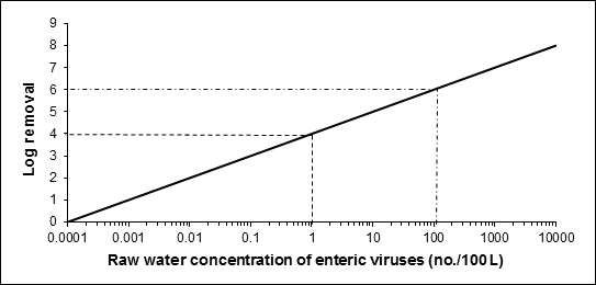
Figure 1 - Text Description
A graph showing the level of treatment required to meet an acceptable level of risk of 10-6 DALY per person per year based on 1 L consumption for concentrations of enteric viruses in a raw water source ranging from 0.0001 viruses per 100 litres to 10000 viruses per 100 litres.
The level of treatment required to meet an acceptable level of risk based on 1 L consumption for enteric virus concentrations ranging from 0.0001 viruses per 100 litres to 10000 viruses per 100 litres in raw water is presented graphically. The x-axis of the graph is the raw water concentrations of enteric viruses per 100 litres using a log scale. The y-axis of the graph is the log removal using a linear scale. The relationship between the values on the x-axis and the values on the y-axis for the risk level of 10-6 DALY per person per year creates a diagonal line. Two examples of treatment requirements are illustrated on the graph using dotted lines. The first example draws a horizontal dotted line from the y-axis at approximately 4 log removal. This dotted line intersects the diagonal line at approximately 1 enteric virus per 100 litres of raw water. The second example draws a horizontal dotted line from the y-axis at approximately 6 log removal. This dotted line intersects the diagonal line at approximately 100 enteric viruses per 100 litres of raw water.
8.4 International considerations
QMRA is increasingly being applied by international agencies and governments at all levels as the foundation for informed decision-making surrounding the health risks from pathogens in drinking water. WHO, the European Commission, the Netherlands, Australia and the United States have all made important advances in QMRA validation and methodology (Staatscourant, 2001; Medema et al., 2006; NRMMC-EPHC, 2006; U.S. EPA, 2006a,b; WHO, 2011). These agencies and governments have adopted approaches that use QMRA to inform the development of health targets (i.e., reference levels of risk or disease) and risk management (e.g., water safety plans, as described in WHO, 2011). Guidance documents on QMRA of drinking water have been published by both the European Commission’s MicroRisk project (Medema et al., 2006), and the U.S. EPA (2014).
The Netherlands and the U.S. EPA provide two examples of QMRA-based regulatory approaches. In the Netherlands, consistent with the WHO approach, water suppliers must conduct a site-specific QMRA on all surface water supplies to determine if the system can meet a specified level of risk. Dutch authorities can also require a QMRA of vulnerable groundwater supplies. In contrast, recent regulatory activity in the United States has seen the U.S. EPA assess the health risks from waterborne pathogens through QMRA and apply this information to set nationwide obligatory treatment performance requirements (U.S. EPA, 2006a, 2006c). In general, drinking water systems must achieve a 4 log removal and/or inactivation of enteric viruses to address risk from enteric viruses (U.S. EPA, 2006a, 2006c).
Health Canada and the Federal-Provincial-Territorial Committee on Drinking Water have chosen the same approach as WHO (2011), providing QMRA-based performance targets as minimum requirements. Site-specific QMRA is also recommended as a tool that can be used as part of a multi-barrier source-to-tap approach. A site-specific QMRA approach offers a number of advantages, including 1) the ability to compare the risk from representative groups of pathogens (e.g., viruses, protozoa, bacteria) in an overall assessment; 2) the transparency of assumptions; 3) the potential to account for variability and uncertainty in estimates; 4) the removal of hidden safety factors (these can be applied as a conscious choice by regulatory authorities at the end of the process, if desired); 5) the site-specific identification of critical control points and limits through sensitivity analysis; and 6) the clear implications of system management on a public health outcome. Further information on using QMRA for site-specific assessments is provided in Health Canada (in preparation).
9.0 Rationale
More than 140 types of enteric viruses are known to infect humans. These pathogens are excreted in the faeces, and sometimes the urine, of infected persons and animals and can potentially be found in source water. Their occurrence in source water varies over time and can be significantly affected by extreme weather or spill events (i.e., increases in virus levels associated with these events). The best way to safeguard against the presence of hazardous levels of enteric viruses in drinking water is based on the application of the multi-barrier approach, including source water protection and adequate treatment, as demonstrated using appropriate process monitoring, followed by the verification of the absence of faecal indicator organisms in the treated water.
The protection of public health is accomplished by setting health-based treatment goals. To set health-based treatment goals, a reference level of risk deemed tolerable or acceptable needs to be determined. The Federal-Provincial-Territorial Committee on Drinking Water has chosen a reference level of risk of 10−6 DALY/person per year, which is consistent with the reference level adopted by the World Health Organization. This is a risk management decision that balances the estimated disease burden from enteric viruses with the lack of information on the prevalence of these pathogens in source waters, limitations in disease surveillance and the variations in performance within different types of water treatment technologies.
The QMRA approach used in this guideline technical document demonstrates that if a source water has a virus concentration of 1/100 L, water treatment (i.e., removal and/or inactivation) would need to consistently achieve at least a 4 log reduction in virus concentration in order to meet the reference level of 10−6 DALY/person per year. Thus, a minimum 4 log removal and/or inactivation of enteric viruseshas been established as a health-based treatment goal for sources vulnerable to virus contamination. Many water sources in Canada, including groundwater, may require more than the minimum treatment goal to meet the reference level of risk. Where possible, watersheds or aquifers that are used as sources of drinking water should be protected from faecal waste.
10.0 References
- Abbaszadegan, M., Stewart, P.W., LeChevallier, M.W. and Gerba, C.P. (1998). Application of PCR technologies for virus detection in groundwater. American Water Works Association, 90740, Denver, Colorado.
- Abbaszadegan, M., Lechevallier, M. and Gerba, C. (2003). Occurrence of viruses in US groundwaters. J. Am. Water Works Assoc., 95(9): 107–120+12.
- Abbaszadegan, M., Mayer, B.K., Ryu, H. and Nwachuku, N. (2007). Efficacy of removal of CCL viruses under enhanced coagulation conditions. Environ. Sci. Technol., 41(3): 971–977.
- Abbaszadegan, M., Monteiro, P., Nwachuku, N., Alum, A. and Ryu, H. (2008). Removal of adenovirus, calicivirus, and bacteriophages by conventional drinking water treatment. J. Environ. Sci. Health Part A Toxic Hazard. Subst. Environ. Eng., 43(2): 171–177.
- Abe, K., Inami, T., Asano, K., Miyoshi, C., Masaki, N., Hayashi, S., Ishikawa, K.-., Takebe, Y., Win, K.M., El-Zayadi, A.R., Han, K.-. and Zhang, D.Y. (1999). TT virus infection is widespread in the general populations from different geographic regions. J. Clin. Microbiol., 37(8): 2703–2705.
- Adham, S.S. and Jacangelo, J.G. (1994). Assessing the reliability of low pressure membrane systems for microbial removal. In: Proceedings of the ASCE Critical Issues in Water and Wastewater Treatment Conference, Boulder, Colorado.
- Adham, S.S., Jacangelo, J.G. and Laine, J-M. (1995). Low pressure membranes: Assessing integrity. J. Am. Water Works Assoc., 87(3): 62–75.
- Ahmed, S.M., Lopman, B.A. and Levy, K. (2013). A systematic review and meta-analysis of the global seasonality of norovirus. Plos One, 8(10).
- Albinana-Gimenez, N., Miagostovich, M.P., Calgua, B., Huguet, J.M., Matia, L. and Girones, R. (2009). Analysis of adenoviruses and polyomaviruses quantified by qPCR as indicators of water quality in source and drinking-water treatment plants. Water Res., 43(7): 2011–2019.
- Albinana-Gimenez, N., Clemente-Casares, P., Calgua, B., Huguet, J.M., Courtois, S. and Girones, R. (2009). Comparison of methods for concentrating human adenoviruses, polyomavirus JC and noroviruses in source waters and drinking water using quantitative PCR. J. Virol. Methods, 158(1–2): 104–109.
- Allen, A. S. (2013). Vulnerability of a fractured bedrock aquifer to emerging sewage-derived contaminants and their use as indicators of virus contamination. Master’s Thesis, University of Guelph, Guelph, Ontario.
- Alspach, B., Delphos, P., Pressman, J., Beaty, J., Cooke, T., Voutchkov, N., Schaefer, J., Noack, R., Marascia, F. and Konstanski, D. (2014). Metrics and methods for MF/UF system optimization. In: Proceedings of the Membrane Technology Conference. American Water Works Association, Denver, Colorado.
- Alvarez, M.E. and O'Brien, R.T. (1982). Mechanisms of inactivation of poliovirus by chlorine dioxide and iodine. Appl. Environ. Microbiol., 44(5): 1064–1071.
- Amburgey, J.E., Amirtharajah, A., Brouckaert, B.M. and Spivey, N.C. (2003). An enhanced backwashing technique for improved filter ripening. J. Am. Water Works Assoc., 95(12): 81–94.
- Amundson, D., Lindholm, C., Goyal, S.M. and Robinson, R.A. (1988). Microbial pollution of well water in southeastern minnesota. J. Environ. Sci. Health Part A Environ. Sci. Eng., 23(5): 453–468.
- Amvrosieva, T.V., Titov, L.P., Mulders, M., Hovi, T., Dyakonova, O.V., Votyakov, V.I., Kvacheva, Z.B., Eremin, V.F., Sharko, R.M., Orlova, S.V., Kazinets, O.N. and Bogush, Z.F. (2001). Viral water contamination as the cause of aseptic meningitis outbreak in Belarus. Cent. Eur. J. Public Health, 9(3): 154–157.
- Anderson, A.D., Heryford, A.G., Sarisky, J.P., Higgins, C., Monroe, S.S., Beard, R.S., Newport, C.M., Cashdollar, J.L., Fout, G.S., Robbins, D.E., Seys, S.A., Musgrave, K.J., Medus, C., Vinjé, J., Bresee, J.S., Mainzer, H.M. and Glass, R.I. (2003). A waterborne outbreak of norwalk-like virus among snowmobilers - Wyoming, 2001. J. Infect. Dis., 187(2): 303–306.
- Anderson, W.B., Deloyde, J.L., Van Dyke, M.I. and Huck, P.M. (2009). Influence of design and operating conditions on the removal of MS2 bacteriophage by pilot-scale multistage slow sand filtration. J. Water Supply Res. Technol. Aqua, 58(7): 450–462.
- Antony, A., Blackbeard, J. and Leslie, G. (2012). Removal efficiency and integrity monitoring techniques for virus removal by membrane processes. Crit. Rev. Environ. Sci. Technol., 42(9): 891–933.
- Aoki, Y., Suto, A., Mizuta, K., Ahiko, T., Osaka, K. and Matsuzaki, Y. (2010). Duration of norovirus excretion and the longitudinal course of viral load in norovirus-infected elderly patients. J. Hosp. Infect., 75(1): 42–46.
- APHA, AWWA and WEF (1998). Standard methods for the examination of water and wastewater. 20th edition. American Public Health Association, American Water Works Association and Water Environment Federation, Washington, DC.
- Armon, R.H. (2015). Ch. 35: Indicators of waterborne viruses. In: Environmental indicators. Armon, R.H. and Hanninen, O. (eds.). Springer, Dordrecht, Netherlands.
- Arnold, W.R. and Rainbow, A.J. (1996). Host cell reactivation of irradiated adenovirus in UV-sensitive chinese hamster ovary cell mutants. Mutagenesis, 11(1): 89–94.
- Ashbolt, N.J., Grabow, W.O.K. and Snozzi, M. (2001). Indicators of microbial water quality. In: Water quality: Guidelines, standards and health—Assessment of risk and risk management for water-related infectious disease. Fewtrell, L. and Bartram, J. (eds.). IWA Publishing on behalf of the World Health Organization, London, United Kingdom.
- ASTM (2014). Standard practices for detecting leaks in reverse osmosis and nanofiltration devices. Designation: D3923-08 (Reapproved 2014). ASTM International, West Conshohocken, Pennsylvania.
- ASTM (2010). Standard practice for integrity testing of water filtration membrane systems. Designation: D6908-06 (Reapproved 2010). ASTM International, West Conshohocken, Pennsylvania.
- ASTM (2004). ASTM D244-92: Standard practice for recovery of enteroviruses from waters. American Society for Testing and Materials, Philadelphia, Pennsylvania.
- Atmar, R.L. and Estes, M.K. (2001). Diagnosis of noncultivatable gastroenteritis viruses, the human caliciviruses. Clin. Microbiol. Rev., 14(1): 15–37.
- Atmar, R.L., Opekun, A.R., Gilger, M.A., Estes, M.K., Crawford, S.E., Neill, F.H. and Graham, D.Y. (2008). Norwalk virus shedding after experimental human infection. Emerg. Infect. Dis., 14(10): 1553–1557.
- Aw, T.G. and Gin, K.Y. (2010). Environmental surveillance and molecular characterization of human enteric viruses in tropical urban wastewaters. J. Appl. Microbiol., 109(2): 716–730.
- AWWA (1999). Waterborne pathogens. AWWA manual of water practices M48. American Water Works Association, Denver, Colorado.
- AWWA (2005). Microfiltration and ultrafiltration membranes for drinking water. AWWA manual of water practices M53. American Water Works Association, Denver, Colorado.
- AWWA (2006). Waterborne pathogens. AWWA manual of water practices M48. 2nd edition. AWWA manual of water practices M48. American Water Works Association, Denver, Colorado.
- AWWA (2011a). Water quality and treatment: A handbook of community water supplies. 6th edition. Edzwald, J.K. (ed.). McGraw-Hill, New York, New York.
- AWWA (2011b). Operational control of coagulation and filtration processes: Manual of water supply practices – M37. American Water Works Association, Denver, Colorado.
- Azadpour-Keeley, A., Faulkner, B.R. and Chen, J. (2003). Movement and longevity of viruses in the subsurface. U.S. Environmental Protection Agency, EPA/540/S-03/500, Cincinnati, Ohio.
- Baer, G.M. and Walker, J.A. (1977). Studies of an outbreak of acute hepatitis A: I. complement level fluctuation. J. Med. Virol., 1(1): 1–7.
- Bales, R.C., Shimin, L., Maguire, K.M., Yahya, M.T., Gerba, C.P. and Harvey, R.W. (1995). Virus and bacteria transport in a sandy aquifer, Cape Cod, Massachusetts. Groundwater, 33(4): 653–661.
- Bales, R.C., Gerba, C.P., Grondin, G.H. and Jensen, S.L. (1989). Bacteriophage transport in sandy soil and fractured tuff. Appl. Environ. Microbiol., 55(8): 2061–2067.
- Bales, R.C., Hinkle, S.R., Kroeger, T.W., Stocking, K. and Gerba, C.P. (1991). Bacteriophage adsorption during transport through porous media: Chemical perturbations and reversibility. Environ. Sci. Technol., 25(12): 2088–2095.
- Bales, R.C., Li, S., Maguire, K.M., Yahya, M.T. and Gerba, C.P. (1993). MS-2 and poliovirus transport in porous media: Hydrophobic effects and chemical perturbations. Water Resour. Res., 29(4): 957–963.
- Bales, R.C., Li, S., Yeh, T.-.J., Lenczewski, M.E. and Gerba, C.P. (1997). Bacteriophage and microsphere transport in saturated porous media: Forced-gradient experiment at Borden, Ontario. Water Resour. Res., 33(4): 639–648.
- Balkin, H.B. and Margolin, A.B. (2010). Detection of poliovirus by ICC/qPCR in concentrated water samples has greater sensitivity and is less costly using BGM cells in suspension as compared to monolayers. Virol. J., 7: 282–422.
- Ball, J.M., Tian, P., Zeng, C.Q., Morris, A.P. and Estes, M.K. (1996). Age-dependent diarrhea induced by a rotaviral nonstructural glycoprotein. Science, 272(5258): 101–104.
- Ballester, N.A., Fontaine, J.H. and Margolin, A.B. (2005). Occurrence and correlations between coliphages and anthropogenic viruses in the Massachusetts Bay using enrichment and ICC-nPCR. J. Water. Health, 3(1): 59–68.
- Banks, W.S.L. and Battigelli, D.A. (2002). Occurrence and distribution of microbiological contamination and enteric viruses in shallow ground water in Baltimore and Harford Counties, Maryland. U.S.G.S., Water resources investigations report 01-4216.
- Banks, W.S.L., Klohe, C.A. and Battigelli, D.A. (2001). Occurrence and distribution of enteric viruses in shallow ground water and factors affecting well vulnerability to microbiological contamination in Worcester and Wicomico Counties, Maryland. U.S.G.S., Water resources investigations report 01-4147.
- Banyai, K., Bogdan, A., Domonkos, G., Kisfali, P., Molnar, P., Toth, A., Melegh, B., Martella, V., Gentsch, J.R. and Szucs, G. (2009). Genetic diversity and zoonotic potential of human rotavirus strains, 2003-2006, Hungary. J. Med. Virol., 81(2): 362–370.
- Batch, L.F., Schulz, C.R. and Linden, K.G. (2004). Evaluating water quality effects on UV disinfection of MS2 coliphage. J. Am. Water Works Assoc., 96(7): 75–87.
- Bauer, R., Dizer, H., Graeber, I., Rosenwinkel, K.H. and Lopez-Pila, J.M. (2011). Removal of bacterial faecal indicators, coliphages and enteric adenoviruses from waters with high faecal pollution by slow sand filtration. Water Res., 45(2): 439–452.
- Baxter, C.S., Hofmann, R., Templeton, M.R., Brown, M. and Andrews, R.C. (2007). Inactivation of adenovirus types 2, 5, and 41 in drinking water by UV light, free chlorine, and monochloramine. J. Environ. Eng., 133(1): 95–103.
- BC Provincial Health Officer (2001). Report on the health of British Columbians. Public Health Officer’s annual report 2000: Drinking water quality in British Columbia—The public health perspective. Ministry of Health Planning, Victoria, B.C.Beck, S.E., Rodriguez, R.A., Linden, K.G., Hargy, T.M., Larason, T.C. and Wright, H.B. (2014). Wavelength dependent UV inactivation and DNA damage of adenovirus as measured by cell culture infectivity and long range quantitative PCR. Environ. Sci. Technol., 48(1): 591–598.
- Beer, K.D., Gargano, J.W., Roberts, V.A., Hill, V.R., Garrison, L.E., Kutty, P.K., Hilborn, E.D., Wade, T.J., Fullerton, K.E. and Yoder, J.S. (2015). Surveillance for waterborne disease outbreaks associated with drinking water - United States, 2011-2012. MMWR Morb. Mortal. Wkly. Rep., 64(31): 842–848.
- Bell, K., LeChevallier, M., Abbaszadegan, M., Amy, G., Sinha, S., Benjamin, M. and Ibrahim, E. (1998). Enhanced and optimized coagulation for particulate and microbial removal. AWWA Research Foundation and American Water Works Association, Denver, Colorado.
- Bellamy, W.D., Hendricks, D.W. and Logsdon, G.S. (1985). Slow sand filtration: Influences of selected process variables. J. Am. Water Works Assoc., 77(12): 62–66.
- Beller, M., Ellis, A., Lee, S.H., Drebot, M.A., Jenkerson, S.A., Funk, E., Sobsey, M.D., Simmons III, O.D., Monroe, S.S., Ando, T., Noel, J., Petric, M., Middaugh, J.P. and Spika, J.S. (1997). Outbreak of viral gastroenteritis due to a contaminated well: International consequences. J. Am. Med. Assoc., 278(7): 563–568.
- Bellou, M.I., Syngouna, V.I., Tselepi, M.A., Kokkinos, P.A., Paparrodopoulos, S.C., Vantarakis, A. and Chrysikopoulos, C.V. (2015). Interaction of human adenoviruses and coliphages with kaolinite and bentonite. Sci. Total Environ., 517: 86–95.
- Bendinelli, M., Pistello, M., Maggi, F., Fornai, C., Freer, G. and Vatteroni, M.L. (2001). Molecular properties, biology, and clinical implications of TT virus, a recently identified widespread infectious agent of humans. Clin. Microbiol. Rev., 14(1): 98–113.
- Berger, P. (1994). Regulation related to groundwater contamination: The draft groundwater disinfection rule. In: Groundwater contamination and control. Zoller, U. (ed.). M. Dekker, New York, pp. 645–659.
- Betanzo, E.W., Hofmann, R., Hu, Z., Baribeau, H. and Alam, Z. (2008). Modeling the impact of microbial intrusion on secondary disinfection in a drinking water distribution system. J. Environ. Eng., 134(4): 231–237.
- Beuret, C. (2003). A simple method for isolation of enteric viruses (noroviruses and enteroviruses) in water. J. Virol. Methods, 107(1): 1–8.
- Biagini, P. (2004). Human circoviruses. Vet. Microbiol., 98(2): 95–101.
- Bitton, G. (1975). Adsorption of viruses onto surfaces in soil and water. Water Res., 9(5–6): 473–484.
- Bitton, G. (1999). Wastewater microbiology. 2nd edition. Wiley-Liss, New York, New York.
- Blackburn, B.G., Craun, G.F., Yoder, J.S., Hill, V., Calderon, R.L., Chen, N., Lee, S.H., Levy, D.A. and Beach, M.J. (2004). Surveillance for waterborne-disease outbreaks associated with drinking water–United States, 2001-2002. MMWR Surveill. Summ., 53(8): 23–45.
- Blanton, L.H., Adams, S.M., Beard, R.S., Wei, G., Bulens, S.K., Widdowson, M.A., Glass, R.I. and Monroe, S.S. (2006). Molecular and epidemiologic trends of caliciviruses associated with outbreaks of acute gastroenteritis in the United States, 2000-2004. J. Infect. Dis., 193(3): 413–421.
- Bloch, A.B., Stramer, S.L., Smith, J.D., Margolis, H.S., Fields, H.A., McKinley, T.W., Gerba, C.P., Maynard, J.E. and Sikes, R.K. (1990). Recovery of hepatitis A virus from a water supply responsible for a common source outbreak of hepatitis A. Am. J. Public Health, 80(4): 428–430.
- Blokker, M., Smeets, P. and Medema, G. (2014). QMRA in the drinking water distribution system. Procedia Eng , pp. 151–159.
- Boccia, D., Tozzi, A.E., Benvon, C., Rizzo, C., Russo, T., Buttinelli, G., Caprioli, A., Marziano, M.L. and Ruggeri, F.M. (2002). Waterborne outbreak of norwalk-like virus gastroenteritis at a tourist resort, Italy. Emerg. Infect. Dis., 8(6): 563–568.
- Boettger, B. (1995). Kaslo waterborne disease outbreak. B.C. Health Dis. Surveill, 4: 122–125.
- Bofill-Mas, S. and Girones, R. (2003). Role of the environment in the transmission of JC virus. J. Neurovirol., 9 Suppl 1: 54–58.
- Bolton, J.R. and Cotton, C.A. (2008). The ultraviolet disinfection handbook. American Water Works Association, Denver, Colorado.
- Bonilla, J.A., Bonilla, T.D., Abdelzaher, A.M., Scott, T.M., Lukasik, J., Solo-Gabriele, H.M. and Palmer, C.J. (2015). Quantification of protozoa and viruses from small water volumes. Int. J. Environ. Res. Public. Health., 12(7): 7118–7132.
- Borchardt, M.A., Bertz, P.D., Spencer, S.K. and Battigelli, D.A. (2003). Incidence of enteric viruses in groundwater from household wells in Wisconsin. Appl. Environ. Microbiol., 69(2): 1172–1180.
- Borchardt, M.A., Haas, N.L. and Hunt, R.J. (2004). Vulnerability of drinking-water wells in La Crosse, Wisconsin, to enteric-virus contamination from surface water contributions. Appl. Environ. Microbiol., 70(10): 5937–5946.
- Borchardt, M.A., Bradbury, K.R., Gotkowitz, M.B., Cherry, J.A. and Parker, B.L. (2007). Human enteric viruses in groundwater from a confined bedrock aquifer. Environ. Sci. Technol., 41(18): 6606–6612.
- Borchardt, M.A., Bradbury, K.R., Alexander, E.C., Kolberg, R.J., Alexander, S.C., Archer, J.R., Braatz, L.A., Forest, B.M., Green, J.A. and Spencer, S.K. (2011). Norovirus outbreak caused by a new septic system in a dolomite aquifer. Ground Water, 49(1): 85–97.
- Borchardt, M.A., Spencer, S.K., Kieke, B.A., Lambertini, E. and Loge, F.J. (2012). Viruses in nondisinfected drinking water from municipal wells and community incidence of acute gastrointestinal illness. Environ. Health Perspect., 120(9): 1272–1279.
- Bosch, A., Pinto, R.M., Comas, J. and Abad, F.X. (2004). Detection of infectious rotaviruses by flow cytometry. Methods Mol. Biol., 268: 61–68.
- Bosch, A., Guix, S., Sano, D. and Pinto, R.M. (2008). New tools for the study and direct surveillance of viral pathogens in water. Curr. Opin. Biotechnol., 19(3): 295–301.
- Boudaud, N., Machinal, C., David, F., Freval-Le Bourdonnec, A., Jossent, J., Bakanga, F., Arnal, C., Jaffrezic, M.P., Oberti, S. and Gantzer, C. (2012). Removal of MS2, qbeta and GA bacteriophages during drinking water treatment at pilot scale. Water Res., 46(8): 2651–2664.
- Bradbury, K.R., Borchardt, M.A., Gotkowitz, M., Spencer, S.K., Zhu, J. and Hunt, R.J. (2013). Source and transport of human enteric viruses in deep municipal water supply wells. Environ. Sci. Technol., 47(9): 4096–4103.
- Bradbury, K.R., Gotkowitz, M.B., Hart, D. J., Eaton, T.T., Cherry, J.A., Parker, B.L. and Borchardt, M.A. (2006). Contaminant transport through aquitards: Technical guidance for aquitard assessment. Awwa Research Foundation, Denver, CO.
- Brassard, J., Seyer, K., Houde, A., Simard, C. and Trottier, Y.L. (2005). Concentration and detection of hepatitis A virus and rotavirus in spring water samples by reverse transcription-PCR. J. Virol. Methods, 123(2): 163–169.
- Bremer, J.E. and Harter, T. (2012). Domestic wells have high probability of pumping septic tank leachate. Hydrol. Earth Syst. Sci., 16(8): 2453–2467.
- Brown, C.M., Cann, J.W., Simons, G., Fankhauser, R.L., Thomas, W., Parashar, U.D. and Lewis, M.J. (2001). Outbreak of norwalk virus in a Carribbean island resort: Application of molecular diagnostics to ascertain the vehicle of infection. Epidemiol. Infect., 126(3): 425–432.
- Brugha, R., Vipond, I.B., Evans, M.R., Sandifer, Q.D., Roberts, R.J., Salmon, R.L., Caul, E.O. and Mukerjee, A.K. (1999). A community outbreak of food-borne small round-structured virus gastroenteritis caused by a contaminated water supply. Epidemiol. Infect., 122(1): 145–154.
- Brunkard, J.M., Ailes, E., Roberts, V.A., Hill, V., Hilborn, E.D., Craun, G.F., Rajasingham, A., Kahler, A., Garrison, L., Hicks, L., Carpenter, J., Wade, T.J., Beach, M.J., Yoder Msw, J.S. and CDC (2011). Surveillance for waterborne disease outbreaks associated with drinking water-United States, 2007-2008. MMWR Surveill. Summ., 60(12): 38–68.
- Candy, D.C. (2007). Rotavirus infection: A systemic illness? PLoS Med., 4(4): e117.
- Cantera, J.L., Chen, W. and Yates, M.V. (2010). Detection of infective poliovirus by a simple, rapid, and sensitive flow cytometry method based on fluorescence resonance energy transfer technology. Appl. Environ. Microbiol., 76(2): 584–588.
- Carlson, G.F.,Jr, Woodard, F.E., Wentworth, D.F. and Sproul, O.J. (1968). Virus inactivation on clay particles in natural waters. J. Water Pollut. Control Fed., 40(2): R89–106.
- Carrique-Mas, J., Andersson, Y., Petersén, B., Hedlund, K.O., Sjögren, N. and Giesecke, J. (2003). A norwalk-like virus waterborne community outbreak in a Swedish village during peak holiday season. Epidemiol. Infect., 131(1): 737–744.
- Carter, M.J. (2005). Enterically infecting viruses: Pathogenicity, transmission and significance for food and waterborne infection. J. Appl. Microbiol., 98(6): 1354–1380.
- Cashdollar, J.L., Brinkman, N.E., Griffin, S.M., McMinn, B.R., Rhodes, E.R., Varughese, E.A., Grimm, A.C., Parshionikar, S.U., Wymer, L. and Fout, G.S. (2013). Development and evaluation of EPA method 1615 for detection of enterovirus and norovirus in water. Appl. Environ. Microbiol., 79(1): 215–223.
- Caul, E.O. (1994). Small round structured viruses: airborne transmission and hospital control. Lancet, 343(8908): 1240–1242.
- Caul, E.O. (1996). Viral gastroenteritis: Small round structured viruses, caliciviruses and astroviruses. part II. the epidemiological perspective. J. Clin. Pathol., 49(12): 959–964.
- Caul, E.O., Ashley, C.R., Darville, J.M. and Bridger, J.C. (1990). Group C rotavirus associated with fatal enteritis in a family outbreak. J. Med.Virol, 30: 201–205.
- CCME (2004). From source to tap: Guidance on the multi-barrier approach to safe drinking water. Canadian Council of Ministers of the Environment, Winnipeg, Manitoba.
- CDC, (2011). Updated norovirus outbreak management and disease prevention guidelines. MMWR Recomm Rep., 60(RR-3): 1–18.
- CDC (2013a). Norovirus clinical overview. Available at: www.cdc.gov/norovirus/hcp/clinical-overview.html.
- CDC (2013b). Surveillance for waterborne disease outbreaks associated with drinking water and other nonrecreational water – United States, 2009-2010. MMWR Morb. Mortal. Wkly. Rep., 62(35): 714–720.
- CDC (2015a). Viral hepatitis – hepatitis A information. Available at: www.cdc.gov/hepatitis/hav/havfaq.htm.
- CDC (2015b). Chapter 19: Rotavirus. In: Epidemiology and prevention of vaccine-preventable diseases. Hamborsky, J., Kroger, A. and Wolfe, S. (eds.). 13th. Public Health Foundation, Washington, DC.
- Chang, J.C., Ossoff, S.F., Lobe, D.C., Dorfman, M.H., Dumais, C.M., Qualls, R.G. and Johnson, J.D. (1985). UV inactivation of pathogenic and indicator microorganisms. Appl. Environ. Microbiol., 49(6): 1361–1365.
- Chao, D.Y., Wei, J.Y., Chang, W.F., Wang, J. and Wang, L.C. (2012). Detection of multiple genotypes of calicivirus infection in asymptomatic swine in Taiwan. Zoonoses Public. Health., 59(6): 434–444.
- Charles, K.J., Shore, J., Sellwood, J., Laverick, M., Hart, A. and Pedley, S. (2009). Assessment of the stability of human viruses and coliphage in groundwater by PCR and infectivity methods. J. Appl. Microbiol., 106(6): 1827-1837.
- Cheetham, S., Souza, M., McGregor, R., Meulia, T., Wang, Q. and Saif, L.J. (2007). Binding patterns of human norovirus-like particles to buccal and intestinal tissues of gnotobiotic pigs in relation to A/H histo-blood group antigen expression. J. Virol., 81(7): 3535–3544.
- Cherry, J.D. (1992). Enteroviruses: Poloviruses (poliomyelitis), coxsackieviruses, echoviruses, and enteroviruses. In: Textbook of pediatric infectious diseases. Feigin, R.D. (ed.). 3rd. W.B. Saunders Co., Philadelphia, Pennsylvania., pp. 3535–3544.
- Cherry, J.A., Parker, B.L., Bradbury, K.R., Eaton, T.T., Gotkowitz, M.B., Hart, D.J. and Borchardt, M.A. (2006). Contaminant transport through aquitards: A state-of-the-science review. Awwa Research Foundation, Denver, Colorado.
- Chevrefils, G., Caron, É., Wright, H., Sakamoto, G., Payment, P., Barbeau, B. and Cairns, B. (2006). UV dose required to achieve incremental log inactivation of bacteria, protozoa and viruses. J. Int. UV Assoc. (IUVA) News, 8: 38–45.
- Chia, J.K. and Chia, A.Y. (2008). Chronic fatigue syndrome is associated with chronic enterovirus infection of the stomach. J. Clin. Pathol., 61(1): 43–48.
- Chiba, S., Sakuma, Y., Kogasaka, R., Akihara, M., Horino, K., Nakao, T. and Fukui, S. (1979). An outbreak of gastroenteritis associated with calicivirus in an infant home. J. Med. Virol., 4(4): 249–254.
- Chiba, S., Nakata, S., Numata-Kinoshita, K. and Honma, S. (2000). Sapporo virus: history and recent findings. J. Infect. Dis., 181(Suppl. 2): S303–S308.
- Chin, J. (2000). Control of communicable diseases manual. 17th edition.. American Public Health Association, Washington, DC.
- Choi, S. and Jiang, S.C. (2005). Real-time PCR quantification of human adenoviruses in urban rivers indicates genome prevalence but low infectivity. Appl. Environ. Microbiol., 71(11): 7426–7433.
- Christensen, J. and Linden, K. (2002). New findings regarding the impacts of suspended particles on UV disinfection of drinking water. In: Proceedings of the Annual Conference of the American Water Works Association, New Orleans, LA. June 16-20.
- Clemente-Casares, P., Pina, S., Buti, M., Jardi, R., Martín, M., Bofill-Mas, S. and Girones, R. (2003). Hepatitis E virus epidemiology in industrialized countries. Emerg. Infect. Dis., 9(4): 448–454.
- Conio, O., Chioetto, M. and Hargesheimer, E. (2002). Organic monitors. In: Online monitoring for drinking water utilities. Hargesheimer, E., Conio, O. and Papovicova, J. (eds.). AWWA Research Foundation, Denver, Colorado, pp. 163–202.
- Cook, N., Bridger, J., Kendall, K., Gomara, M.I., El-Attar, L. and Gray, J. (2004). The zoonotic potential of rotavirus. J. Infect., 48(4): 289–302.
- Cornwell, D.A. and MacPhee, M.J. (2001). Effects of spent filter backwash recycle on cryptosporidium removal. J. Am. Water Works Assoc., 93(4): 153–162.
- Corsi, S.R., Borchardt, M.A., Spencer, S.K., Hughes, P.E. and Baldwin, A.K. (2014). Human and bovine viruses in the Milwaukee River watershed: Hydrologically relevant representation and relations with environmental variables. Sci. Total Environ., 490: 849–860.
- Cotton, C.A., Linden, K.G., Schmelling, D.C., Bell, C. and Landis, H. (2001). The development of the UV dose tables for LT2ESWTR implementation. First International Congress on Ultraviolet Technologies, Washington, DC.
- Craun, M.F., Craun, G.F., Calderon, R.L. and Beach, M.J. (2006). Waterborne outbreaks reported in the United States. J. Water. Health., 4 Suppl 2: 19–30.
- Cromeans, T.L., Kahler, A.M. and Hill, V.R. (2010). Inactivation of adenoviruses, enteroviruses, and murine norovirus in water by free chlorine and monochloramine. Appl. Environ. Microbiol., 76(4): 1028–1033.
- Crowe, A.S., Schaefer, K.A., Kohut, A., Shikaze, S.G. and Ptacek, C.J. (2003). Linking water science to policy: groundwater quality. Canadian Council of Ministers of the Environment, Winnipeg, Manitoba.
- Curriero, F.C., Patz, J.A., Rose, J.B. and Lele, S. (2001). The association between extreme precipitation and waterborne disease outbreaks in the United States, 1948-1994. Am. J. Public Health, 91(8): 1194–1199.
- De Serres, G., Cromeans, T.L., Levesque, B., Brassard, N., Barthe, C., Dionne, M., Prud’homme, H., Paradis, D., Shapiro, C.N., Nainan, O.V. and Margolis, H.S. (1999). Molecular confirmation of hepatitis A virus from well water: Epidemiology and public health implications. J. Infect. Dis., 179: 37–43.
- DeBorde, D.C., Woessner, W.W., Lauerman, B. and Ball, P.N. (1998). Virus occurrence and transport in a school septic system and unconfined aquifer. Ground Water, 36(5): 825–834.
- DeBorde, D.C., Woessner, W.W., Kiley, Q.T. and Ball, P. (1999). Rapid transport of viruses in a floodplain aquifer. Water Res., 33(10): 2229–2238.
- Dechesne, M. and Soyeux, E. (2007). Assessment of source water pathogen contamination. J. Water Health., 5 Suppl 1: 39–50.
- Deere, D., Stevens, M., Davison, A., Helm, G. and Dufour, A. (2001). Management strategies. Fewtrell, L. and Bartram, J. (eds.). IWA Publishing, London, United Kingdom.
- De Roda Husman, A.M., Lodder, W.J., Rutjes, S.A., Schijven, J.F. and Teunis, P.F.M. (2009). Long-term inactivation study of three enteroviruses in artificial surface and groundwaters, using PCR and cell culture. Appl. Environ. Microbiol., 75(4): 1050–1057.
- Di Giovanni, G.D., Hashemi, F.H., Shaw, N.J., Abrams, F.A., LeChevallier, M.W. and Abbaszadegan, M. (1999). Detection of infectious cryptosporidium parvum oocysts in surface and filter backwash water samples by immunomagnetic separation and integrated cell culture-PCR. Appl. Environ. Microbiol., 65(8): 3427–3432.
- Diniz-Mendes, L., Paula, V.S., Luz, S.L. and Niel, C. (2008). High prevalence of human torque teno virus in streams crossing the city of Manaus, Brazilian Amazon. J. Appl. Microbiol., 105(1): 51–58.
- Divizia, M., Gabrieli, R., Donia, D., Macaluso, A., Bosch, A., Guix, S., Sanchez, G., Villena, C., Pinto, R.M., Palombi, L., Buonuomo, E., Cenko, F., Leno, L., Bebeci, D. and Bino, S. (2004). Waterborne gastroenteritis outbreak in Albania. Water Sci. Technol., 50(1): 57–61.
- Dizer, H., Grutzmacher, G., Bartel, H., Wiese, H.B., Szewzyk, R. and Lopez-Pila, J.M. (2004). Contribution of the colmation layer to the elimination of coliphages by slow sand filtration. Water Sci. Technol., 50(2): 211–214.
- Dong, Y., Kim, J. and Lewis, G.D. (2010). Evaluation of methodology for detection of human adenoviruses in wastewater, drinking water, stream water and recreational waters. J. Appl. Microbiol., 108(3): 800–809.
- Dorner, S.M., Anderson, W.B., Gaulin, T., Candon, H.L., Slawson, R.M., Payment, P. and Huck, P.M. (2007). Pathogen and indicator variability in a heavily impacted watershed. J. Water Health, 5(2): 241–257.
- Doro, R., Farkas, S.L., Martella, V. and Banyai, K. (2015). Zoonotic transmission of rotavirus: Surveillance and control. Expert Rev. Anti Infect. Ther., 13(11): 1337–1350.
- Drayna, P., McLellan, S.L., Simpson, P., Li, S-H. and Gorelick, M.H. (2010). Association between rainfall and pediatric emergency department visits for acute gastrointestinal illness. Environ. Health Perspect., 118(10): 1439–1443.
- Duboise, S.M., Moore, B.E. and Sagik, B.P. (1976). Poliovirus survival and movement in a sandy forest soil. Appl. Environ. Microbiol., 31(4): 536–543.
- Edge, T.A., Khan, I.U., Bouchard, R., Guo, J., Hill, S., Locas, A., Moore, L., Neumann, N., Nowak, E., Payment, P., Yang, R., Yerubandi, R. and Watson, S. (2013). Occurrence of waterborne pathogens and escherichia coli at offshore drinking water intakes in Lake Ontario. Appl. Environ. Microbiol., 79(19): 5799–5813.
- Eischeid, A.C. (2009). Fundamental mechanisms in the extreme UV resistance of adenovirus. Doctoral dissertation. Duke University. Available at: http://dukespace.lib.duke.edu/dspace/bitstream/handle/10161/1256/D_Eischeid_Anne_a_200904.pdf?sequence=1
- ElHadidy, A.M., Peldszus, S. and Van Dyke, M.I. (2013). An evaluation of virus removal mechanisms by ultrafiltration membranes using MS2 and fx174 bacteriophage. Sep. Purif. Technol., 120: 215–223.
- ElHadidy, A.M., Peldszus, S. and Van Dyke, M.I. (2014). Effect of hydraulically reversible and hydraulically irreversible fouling on the removal of MS2 and fX174 bacteriophage by an ultrafiltration membrane. Water Res., 61: 297–307.
- Emelko, M.B., Schmidt, P.J. and Roberson, J.A. (2008). Quantification of uncertainty in microbial data - reporting and regulatory implications. J. Am. Water Works Assoc., 100(3): 94–104+14.
- Emelko, M.B., Schmidt, P.J. and Reilly, P.M. (2010). Particle and microorganism enumeration data: Enabling quantitative rigor and judicious interpretation. Environ. Sci. Technol., 44(5): 1720–1727.
- Engelbrecht, R.S., Weber, M.J., Salter, B.L. and Schmidt, C.A. (1980). Comparative inactivation of viruses by chlorine. Appl. Environ. Microbiol., 40(2): 249–256.
- EPCOR (2010). Annual quality assurrance report. Edmonton, Alberta.
- EPCOR (2011). Annual quality assurrance report. Edmonton, Alberta.
- Espinosa, A.C., Mazari-Hiriart, M., Espinosa, R., Maruri-Avidal, L., Méndez, E. and Arias, C.F. (2008). Infectivity and genome persistence of rotavirus and astrovirus in groundwater and surface water. Water Res., 42(10–11): 2618–2628.
- Estes, M.K. and Kapikian, A.Z. (2007). Rotaviruses. 5th. Knipe, D.M. and Howley, P.M. (eds.). Lippincott Williams and Wilkins, Philadelphia, Pennsylvania.
- Estes, M.K. and Greenberg, H.B. (2013). Rotaviruses. In: Fields virology. Knipe, D.M. and Howley, P.M. (eds.). 6th. Wolters Kluwer Health/Lippincott Williams & Wilkins, Philadelphia, Pennsylvania., pp. 1347–1401.
- Faleye, T.O.C., Adewumi, M.O. and Adeniji, J.A. (2016). Defining the enterovirus diversity landscape of a faecal sample: a methodological challenge? Viruses, 8(1).
- Farkas, T., Zhong, W.M., Jing, Y., Huang, P.W., Espinosa, S.M., Martinez, N., Morrow, A.L., Ruiz-Palacios, G.M., Pickering, L.K. and Jiang, X. (2004). Genetic diversity among sapoviruses. Arch. Virol., 149(7): 1309–1323.
- FDA (2012). Hepatitis A virus. In: Bad bug book, foodborne pathogenic microorganisms and natural toxins. Second edition..U.S. Food and Drug Administration. pp. 174.
- Feffer, A., Baker, D., Moore, R., Wagner, T. and Gresehover, B. (2016). Remote data monitoring improves distribution system efficiency and maintenance. Opflow, 42(2): 10–14.
- Fiksdal, L. and Leiknes, T. (2006). The effect of coagulation with MF/UF membrane filtration for the removal of virus in drinking water. J. Membr. Sci., 279(1–2): 364–371.
- Finkbeiner, S.R., Holtz, L.R., Jiang, Y., Rajendran, P., Franz, C.J., Zhao, G., Kang, G. and Wang, D. (2009a). Human stool contains a previously unrecognized diversity of novel astroviruses. Virol. J., 6: 161.
- Finkbeiner, S.R., Le, B.M., Holtz, L.R., Storch, G.A. and Wang, D. (2009b). Detection of newly described astrovirus MLB1 in stool samples from children. Emerg. Infect. Dis., 15(3): 441–444.
- Fiore, A.E. (2004). Hepatitis A transmitted by food. Clin. Infect. Dis., 38(5): 705–715.
- Fisher, I., Angles, M., Chandy, J., Cox, P., Warnecke, M., Kastl, G. and Jegatheesan, V. (2000). Biofilms - a sticky situation for drinking water? Water (Australia), 27(2): 33–37.
- Fong, T.T. and Lipp, E.K. (2005). Enteric viruses of humans and animals in aquatic environments: Health risks, detection, and potential water quality assessment tools. Microbiol. Mol. Biol. Rev., 69(2): 357–371.
- Fong, T.T., Griffin, D.W. and Lipp, E.K. (2005). Molecular assays for targeting human and bovine enteric viruses in coastal waters and their application for library-independent source tracking. Appl. Environ. Microbiol., 71(4): 2070–2078.
- Fong, T.T., Mansfield, L.S., Wilson, D.L., Schwab, D.J., Molloy, S.L. and Rose, J.B. (2007). Massive microbiological groundwater contamination associated with a waterborne outbreak in Lake Erie, South Bass Island, Ohio. Environ. Health Perspect., 115(6): 856–864.
- Fongaro, G., Nascimento, M.A., Rigotto, C., Ritterbusch, G., da Silva, A.D., Esteves, P.A. and Barardi, C.R. (2013). Evaluation and molecular characterization of human adenovirus in drinking water supplies: Viral integrity and viability assays. Virol. J., 10: 166.
- Fongaro, G., Padilha, J., Schissi, C.D., Nascimento, M.A., Bampi, G.B., Viancelli, A. and Barardi, C.R. (2015). Human and animal enteric virus in groundwater from deep wells, and recreational and network water. Environ. Sci. Pollut. Res. Int., 22(24): 20060–20066.
- Fout, G.S., Martinson, B.C., Moyer, M.W.N. and Dahling, D.R. (2003). A multiplex reverse transcription-PCR method for detection of human enteric viruses in groundwater. Appl. Environ. Microbiol., 69(6): 3158–3164.
- Fout, G.S., Cashdollar, J.L., Varughese, E.A., Parshionikar, S.U. and Grimm, A.C. (2015). EPA method 1615. measurement of enterovirus and norovirus occurrence in water by culture and RT-qPCR. I. collection of virus samples. J. Vis. Exp., (97). doi(97): 10.3791/52067.
- Francy, D.S., Stelzer, E.A., Brady, A.M., Huitger, C., Bushon, R.N., Ip, H.S., Ware, M.W., Villegas, E.N., Gallardo, V. and Lindquist, H.D. (2013). Comparison of filters for concentrating microbial indicators and pathogens in lake water samples. Appl. Environ. Microbiol., 79(4): 1342–1352.
- Francy, D.S., Bushon, R.N., Stopar, J., Luzano, E.J. and Fout, G.S. (2004). Environmental factors and chemical and microbiological water-quality constituents related to the presence of enteric viruses in ground water from small public water supplies in Southeastern Michigan. U.S.G.S., Scientific investigations report 2004–5219.
- FSA (2000). A report of the study of infectious intestinal disease in England. Food Standards Agency, HMSO, London, United Kingdom.
- Fuhrman, J.A., Liang, X. and Noble, R.T. (2005). Rapid detection of enteroviruses in small volumes of natural waters by real-time quantitative reverse transcriptase PCR. Appl. Environ. Microbiol., 71(8): 4523–4530.
- Gabbay, Y.B., Borges, A.A., Oliveira, D.S., Linhares, A.C., Mascarenhas, J.D.P., Barardi, C.R.M., Simões, C.M.O., Wang, Y., Glass, R.I. and Jiang, B. (2008). Evidence for zoonotic transmission of group C rotaviruses among children in Belém, Brazil. J. Med. Virol., 80(9): 1666–1674.
- Gale, P. (1996). Developments in microbiological risk assessment models for drinking water-a short review. J. Appl. Bacteriol., 81(4): 403–410.
- Gallimore, C.I., Iturriza-Gomara, M., Lewis, D., Cubitt, D., Cotterill, H. and Gray, J.J. (2006). Characterization of sapoviruses collected in the united kingdom from 1989 to 2004. J. Med. Virol., 78(5): 673–682.
- Gelting, R., Sarisky, J., Selman, C., Otto, C., Higgins, C., Bohan, P.O., Buchanan, S.B. and Meehan, P.J. (2005). Use of a systems-based approach to an environmental health assessment for a waterborne disease outbreak investigation at a snowmobile lodge in Wyoming. Int. J. Hyg. Environ. Health, 208(1–2): 67–73.
- Gerba, C.P. (1984). Applied and theoretical aspects of virus adsorption to surfaces. Adv. Appl. Microbiol., 30: 133–168.
- Gerba, C.P. and Bitton, G. (1984). Microbial pollutants: Their survival and transport pattern to groundwater. In: Groundwater pollution microbiology. Bitton, G. and Gerba, C.P. (eds.). John Wiley & Sons, New York, New York, pp. 65–88.
- Gerba, C.P., Goyal, S.M., LaBelle, R.L. and Bodgan, G.F. (1979). Failure of indicator bacteria to reflect the occurrence of enteroviruses in marine waters. Am. J. Public Health, 69(11): 1116–1119.
- Gerba, C.P., Goyal, S.M., Cech, I. and Bogdan, G.F. (1981). Quantitative assessment of the adsorptive behavior of viruses to soils. Environ. Sci. Technol., 15(8): 940–944.
- Gerba, C.P., Riley, K.R., Nwachuku, N., Ryu, H. and Abbaszadegan, M. (2003). Removal of encephalitozoon intestinalis, calicivirus, and coliphages by conventional drinking water treatment. J. Environ. Sci. Health. A. Tox. Hazard. Subst. Environ. Eng., 38(7): 1259–1268.
- Gerrity, D., Ryu, H., Crittenden, J. and Abbaszadegan, M. (2008). UV inactivation of adenovirus type 4 measured by integrated cell culture qPCR. J. Environ. Sci. Health. A. Tox. Hazard. Subst. Environ. Eng., 43(14): 1628–1638.
- Giammanco, G.M., Di Bartolo, I., Purpari, G., Costantino, C., Rotolo, V., Spoto, V., Geraci, G., Bosco, G., Petralia, A., Guercio, A., Macaluso, G., Calamusa, G., De Grazia, S., Ruggeri, F.M., Vitale, F., Maida, C.M. and Mammina, C. (2014). Investigation and control of a norovirus outbreak of probable waterborne transmission through a municipal groundwater system. J. Water Health, 12(3): 452–464.
- Gibson, K.E. and Schwab, K.J. (2011). Detection of bacterial indicators and human and bovine enteric viruses in surface water and groundwater sources potentially impacted by animal and human wastes in lower Yakima Valley, Washington. Appl. Environ. Microbiol., 77(1): 355–362.
- Giles, J.P., Liebhaber, H., Krugman, S. and Lattimer, C. (1964). Early viremia and viruria in infectious hepatitis. Virology, 24: 107–108.
- Glass, R.I., Kilgore, P.E., Holman, R.C., Jin, S., Smith, J.C., Woods, P.A., Clarke, M.J., Ho, M.S. and Gentsch, J.R. (1996). The epidemiology of rotavirus diarrhea in the United States: Surveillance and estimates of disease burden. J. Infect. Dis., 174 Suppl 1: S5-11.
- Gleeson, T., Novakowski, K. and Kurt Kyser, T. (2009). Extremely rapid and localized recharge to a fractured rock aquifer. J. Hydrol., 376(3–4): 496–509.
- Gofti-Laroche, L., Gratacap-Cavallier, B., Demanse, D., Genoulaz, O., Seigneurin, J.M. and Zmirou, D. (2003). Are waterborne astrovirus implicated in acute digestive morbidity (E.M.I.R.A. study)? J. Clin. Virol., 27(1): 74–82.
- Gordon, C. and Toze, S. (2003). Influence of groundwater characteristics on the survival of enteric viruses. J. Appl. Microbiol., 95(3): 536–544.
- Goyal, S.M. and Gerba, C.P. (1979). Comparative adsorption of human enteroviruses, simian rotavirus, and selected bacteriophages to soils. Appl. Environ. Microbiol., 38(2): 241–247.
- Grabow, W.O.K. (2001). Bacteriophages: update on application as models for viruses in water. Water SA, 27(2): 251–268.
- Gray, J.J., Wreghitt, T.G., Cubitt, W.D. and Elliot, P.R. (1987). An outbreak of gastroenteritis in a home for the elderly associated with astrovirus type 1 and human calicivirus. J. Med. Virol., 23(4): 377–381.
- Gray, J.J., Green, J., Cunliffe, C., Gallimore, C., Lee, J.V., Neal, K. and Brown, D.W.G. (1997). Mixed genogroup SRSV infections among a party of canoeists exposed to contaminated recreational water. J. Med. Virol., 52(4): 425–429.
- Greenberg, H.B., Wyatt, R.G. and Kapikian, A.Z. (1979). Norwalk virus in vomitus. Lancet, 1(8106): 55.
- Greening, G.E., Hewitt, J. and Lewis, G.D. (2002). Evaluation of integrated cell culture-PCR (C-PCR) for virological analysis of environmental samples. J. Appl. Microbiol., 93(5): 745–750.
- Griffin, D.W., Gibson, C.J., Lipp, E.K., Riley, K., Paul, J.H. and Rose, J.B. (1999). Detection of viral pathogens by reverse transcriptase PCR and of microbial indicators by standard methods in the canals of the Florida Keys. Appl. Environ. Microbiol., 65(9): 4118–4125.
- Griffin, D.W., Donaldson, K.A., Paul, J.H. and Rose, J.B. (2003). Pathogenic human viruses in coastal waters. Clin. Microbiol. Rev., 16(1): 129–143.
- Griffin, J.S., Plummer, J.D. and Long, S.C. (2008). Torque teno virus: An improved indicator for viral pathogens in drinking waters. Virol. J., 5: 112.
- Gunnarsdottir, M.J., Gardarsson, S.M. and Andradottir, H.O. (2013). Microbial contamination in groundwater supply in a cold climate and coarse soil: Case study of norovirus outbreak at lake Mývatn, Iceland. Hydrol. Res., 44(6): 1114–1128.
- Guo, H., Wyart, Y., Perot, J., Nauleau, F. and Moulin, P. (2010a). Low-pressure membrane integrity tests for drinking water treatment: A review. Water Res., 44(1): 41–57.
- Guo, H., Chu, X. and Hu, J. (2010b). Effect of host cells on low- and medium-pressure UV inactivation of adenoviruses. Appl. Environ. Microbiol., 76(21): 7068–7075.
- Guthmann, J.P., Klovstad, H., Boccia, D., Hamid, N., Pinoges, L., Nizou, J.Y., Tatay, M., Diaz, F., Moren, A., Grais, R.F., Ciglenecki, I., Nicand, E. and Guerin, P.J. (2006). A large outbreak of hepatitis E among a displaced population in Darfur, Sudan, 2004: The role of water treatment methods. Clin. Infect. Dis., 42(12): 1685–1691.
- Haas, C.N., Rose, J.B. and Gerba, C.P. (1999). Quantitative microbial risk assessment. John Wiley, New York, New York.
- Haas, C.N., Rose, J.B. and Gerba, C.P. (2014). Quantitative microbial risk assessment. Second edition. John Wiley, New York, New York.
- Häfliger, D., Hubner, P. and Luthy, J. (2000). Outbreak of viral gastroenteritis due to sewage-contaminated drinking water. Int. J. Food Microbiol., 54(1–2): 123–126.
- Haines, K.E. and O’Brien, R.T. (1979). The survival of enteric viruses in septic tanks and septic tank drain fields. New Mexico Water Resources Research Institute, New Mexico State University, New Mexico.
- Halbur, P.G., Kasorndorkbua, C., Gilbert, C., Guenette, D., Potters, M.B., Purcell, R.H., Emerson, S.U., Toth, T.E. and Meng, X.J. (2001). Comparative pathogenesis of infection of pigs with hepatitis E viruses recovered from a pig and a human. J. Clin. Microbiol., 39(3): 918–923.
- Hamano, M., Kuzuya, M., Fujii, R., Ogura, H., Mori, T., Nakayama, T., Yuen, E., Katayama, K., Mitsunobu, Y. and Inoue, K. (1999). Outbreak of acute gastroenteritis caused by human group C rotavirus in a primary school. Jpn. J. Infect. Dis., 52(4): 170–171.
- Hansman, G.S., Sano, D., Ueki, Y., Imai, T., Oka, T., Katayama, K., Takeda, N. and Omura, T. (2007). Sapovirus in water, Japan. Emerg. Infect. Dis., 13(1): 133–135.
- Haramoto, E., Katayama, H. and Ohgaki, S. (2004). Detection of noroviruses in tap water in Japan by means of a new method for concentrating enteric viruses in large volumes of freshwater. Appl. Environ. Microbiol., 70(4): 2154–2160.
- Haramoto, E., Katayama, H., Oguma, K. and Ohgaki, S. (2005a). Application of cation-coated filter method to detection of noroviruses, enteroviruses, adenoviruses, and torque teno viruses in the Tamagawa River in Japan. Appl. Environ. Microbiol., 71(5): 2403–2411.
- Haramoto, E., Katayama, H., Oguma, K., Yamashita, H., Nakajima, E. and Ohgaki, S. (2005b). One-year monthly monitoring of torque teno virus (TTV) in wastewater treatment plants in Japan. Water Res., 39(10): 2008–2013.
- Haramoto, E., Kitajima, M., Katayama, H. and Ohgaki, S. (2010). Real-time PCR detection of adenoviruses, polyomaviruses, and torque teno viruses in river water in Japan. Water Res., 44(6): 1747–1752.
- Harman, J., Robertson, W.D., Cherry, J.A. and Zanini, L. (1996). Impacts on a sand aquifer from an old septic system: Nitrate and phosphate. Ground Water, 34(6): 1105–1114.
- Harrington, G.W., Chen, H., Harris, A.J., Xagoraraki, I., Battigelli, D.A. and Standridge, J.H. (2001). Removal of emerging waterborne pathogens. AWWA Research Foundation and American Water Works Association, Denver, Colorado.
- Harrington, G.W., Xagoraraki, I., Assavasilavasukul, P. and Standridge, J.H. (2003). Effect of filtration conditions on removal of emerging waterborne pathogens. J. Am. Water Works Assoc., 95(12): 95–104.
- Hartmann, N.M., Dartscht, M., Szewzyk, R. and Selinka, H-C. (2013). Monitoring of adenovirus serotypes in environmental samples by combined PCR and melting point analyses. Virol. J., 10: 190.
- Harvey, R.W., Metge, D.W., LeBlanc, D.R., Underwood, J., Aiken, G.R., Butler, K., McCobb, T.D. and Jasperse, J. (2015). Importance of the colmation layer in the transport and removal of cyanobacteria, viruses, and dissolved organic carbon during natural lake-bank filtration. J. Environ. Qual., 44(5): 1413–1423.
- Hata, A., Kitajima, M. and Katayama, H. (2013). Occurrence and reduction of human viruses, F-specific RNA coliphage genogroups and microbial indicators at a full-scale wastewater treatment plant in Japan. J. Appl. Microbiol., 114(2): 545–554.
- Hata, A., Katayama, H., Kojima, K., Sano, S., Kasuga, I., Kitajima, M. and Furumai, H. (2014). Effects of rainfall events on the occurrence and detection efficiency of viruses in river water impacted by combined sewer overflows. Sci. Total Environ., 468–469: 757–763.
- Hauri, A.M., Schimmelpfennig, M., Walter-Domes, M., Letz, A., Diedrich, S., Lopez-Pila, J. and Schreier, E. (2005). An outbreak of viral meningitis associated with a public swimming pond. Epidemiol. Infect., 133(2): 291–298.
- Havelaar, A.H. (1987). Bacteriophages as model organisms in water treatment. Microbiol. Sci., 4(12): 362–364.
- Havelaar, A. and Melse, J.M. (2003). Quantifying public health risk in the WHO guidelines for drinking-water quality: A burden of disease approach. Rijkinstituut voor Volskgezondheid en Milieu, RIVM Report 734301022, Bilthoven, Netherlands.
- Havelaar, A.H., Van Olphen, M. and Drost, Y.C. (1993). F-specific RNA bacteriophages are adequate model organisms for enteric viruses in fresh water. Appl. Environ. Microbiol., 59(9): 2956–2962.
- Havelaar, A.H., Van Olphen, M. and Schijven, J.F. (1995). Removal and inactivation of viruses by drinking water treatment processes under full scale conditions. Water Sci. Technol., 31(5–6): 55–62.
- He, X.Q., Cheng, L., Zhang, D.Y., Xie, X.M., Wang, D.H. and Wang, Z. (2011). One-year monthly survey of rotavirus, astrovirus and norovirus in three sewage treatment plants (STPs) in Beijing, China and associated health risk assessment. Water Sci. Technol., 64(6): 1202–1210.
- Health and Welfare Canada (1990). Foodborne disease in Canada, 10-year summary 1975-1984. Health Protection Branch, Ottawa, Ontario.
- Health Canada (1994). Foodborne and waterborne disease in Canada, annual summary 1987. Health Protection Branch, Ottawa, Ontario.
- Health Canada (1996). Foodborne and waterborne disease in Canada, annual summaries: 1988–1989. Health Protection Branch, Ottawa, Ontario.
- Health Canada (2006). Guidelines for Canadian drinking water quality: Guideline technical document—Trihalomethanes. Water Quality and Health Bureau, Healthy Environments and Consumer Safety Branch, Health Canada, Ottawa, Ontario.
- Health Canada (2008a). Guidelines for Canadian drinking water quality: Guideline technical document—Chlorite and chlorate. Water, Air and Climate Change Bureau, Healthy Environments and Consumer Safety Branch, Health Canada, Ottawa, Ontario.
- Health Canada (2008b). Guidelines for Canadian drinking water quality: Guideline technical document—Haloacetic acids. Water, Air and Climate Change Bureau, Healthy Environments and Consumer Safety Branch, Ottawa, Ontario.
- Health Canada (2011). Guidelines for Canadian drinking water quality: Guideline technical document — N-nitrosodimethylamine (NDMA). Water, Air and Climate Change Bureau, Healthy Environments and Consumer Safety Branch, Health Canada, Ottawa, Ontario.
- Health Canada (2012a). Guidelines for Canadian drinking water quality: Guideline technical document—Escherichia coli. Water, Air and Climate Change Bureau, Healthy Environments and Consumer Safety Branch, Health Canada, Ottawa, Ontario.
- Health Canada (2012b). Guidelines for canadian drinking water quality: Guideline technical document—Total coliforms. Water, Air and Climate Change Bureau, Healthy Environments and Consumer Safety Branch, Health Canada, Ottawa, Ontario.
- Health Canada (2012c). Guidelines for Canadian drinking water quality: Guideline technical document – Enteric protozoa: Giardia and cryptosporidium. Water, Air and Climate Change Bureau, Healthy Environments and Consumer Safety Branch, Health Canada, Ottawa, Ontario.
- Health Canada (2012d). Guidelines for Canadian drinking water quality: Guideline technical document — Turbidity. Water and Air Quality Bureau, Healthy Environments and Consumer Safety Branch, Health Canada, Ottawa, Ontario.
- Health Canada (2016). Guidelines for Canadian drinking water quality: Guideline technical document — Bromate. Water and Air Quality Bureau, Healthy Environments and Consumer Safety Branch, Health Canada, Ottawa, Ontario.
- Hellmer, M., Paxeus, N., Magnius, L., Enache, L., Arnholm, B., Johansson, A., Bergstrom, T. and Norder, H. (2014). Detection of pathogenic viruses in sewage provided early warnings of hepatitis A virus and norovirus outbreaks. Appl. Environ. Microbiol., 80(21): 6771–6781.
- Hendricks, D.W., Clunie, W.F., Sturbaum, G.D., Klein, D.A., Champlin, T.L., Kugrens, P., Hirsch, J., McCourt, B., Nordby, G.R., Sobsey, M.D., Hunt, D.J. and Allen, M.J. (2005). Filtration removals of microorganisms and particles. J. Environ. Eng., 131(12): 1621–1632.
- Herrmann, J.E., Kostenbader, K.D.,Jr and CLIVER, D.O. (1974). Persistence of enteroviruses in lake water. Appl. Microbiol., 28(5): 895–896.
- Hewitt, J., Bell, D., Simmons, G.C., Rivera-Aban, M., Wolf, S. and Greening, G.E. (2007). Gastroenteritis outbreak caused by waterborne norovirus at a New Zealand ski resort. Appl. Environ. Microbiol., 73(24): 7853–7857.
- Hijnen, W.A.M. (2011). Chapter 12: Quantitative methods to assess capacity of water treatment processes to eliminate micro-organisms. In: Quantitative methods to assess capacity of water treatment to eliminate micro-organisms. IWA Publishing, London, United Kingdom, pp. 162–166.
- Hijnen, W.A. and Medema, G.J. (2010). Elimination of micro-organisms by drinking water treatment processes—A review. KWR Watercycle Research Institute. IWA Publishing, London, United Kingdom.
- Hijnen, W.A., Schijven, J.F., Bonne, P., Visser, A. and Medema, G.J. (2004a). Elimination of viruses, bacteria and protozoan oocysts by slow sand filtration. Water Sci. Technol., 50(1): 147–154.
- Hijnen, W.A.M., Van Der Veer, A.J., Beerendonk, E.F. and Medema, G.J. (2004b). Increased resistance of environmental anaerobic spores to inactivation by uv. Water Science and Technology: Water Supply, 4(2): 55–61.
- Hijnen, W.A., Beerendonk, E.F. and Medema, G.J. (2006). Inactivation credit of UV radiation for viruses, bacteria and protozoan (oo)cysts in water: A review. Water Res., 40(1): 3–22.
- Hijnen, W.A., Suylen, G.M., Bahlman, J.A., Brouwer-Hanzens, A. and Medema, G.J. (2010). GAC adsorption filters as barriers for viruses, bacteria and protozoan (oo)cysts in water treatment. Water Res., 44(4): 1224–1234.
- Hill, V.R., Polaczyk, A.L., Hahn, D., Narayanan, J., Cromeans, T.L., Roberts, J.M. and Amburgey, J.E. (2005). Development of a rapid method for simultaneous recovery of diverse microbes in drinking water by ultrafiltration with sodium polyphosphate and surfactants. Appl. Environ. Microbiol., 71(11): 6878–6884.
- Hill, V.R., Kahler, A.M., Jothikumar, N., Johnson, T.B., Hahn, D. and Cromeans, T.L. (2007). Multistate evaluation of an ultrafiltration-based procedure for simultaneous recovery of enteric microbes in 100-liter tap water samples. Appl. Environ. Microbiol., 73(13): 4218–4225.
- Hoa Tran, T.N., Trainor, E., Nakagomi, T., Cunliffe, N.A. and Nakagomi, O. (2013). Molecular epidemiology of noroviruses associated with acute sporadic gastroenteritis in children: global distribution of genogroups, genotypes and GII.4 variants. J. Clin. Virol., 56(3): 185–193.
- Hoebe, C.J., Vennema, H., de Roda Husman, A.M. and van Duynhoven, Y.T. (2004). Norovirus outbreak among primary schoolchildren who had played in a recreational water fountain. J. Infect. Dis., 189(4): 699–705.
- Hoff, J.C. (1986). Inactivation of microbial agents by chemical disinfectants. U.S. Environmental Protection Agency, EPA/600/S2-86/067, Cincinnati, Ohio.
- Hofmann, R. (2015). UV dose requirements for enteric viruses. Report for Water, Air and Climate Change Bureau, Healthy Environments and Consumer Safety Branch, Health Canada, Ottawa, Ontario.
- Hollinger, F.B. and Emerson, S.U. (2007). Hepatitis A virus. Knipe, D.M. and Howley, P.M. (eds.). 5th edition. Lippincott Williams and Wilkins, Philadelphia, Pennsylvania.
- Hörman, A., Rimhanen-Finne, R., Maunula, L., Von Bonsdorff, C., Torvela, N., Heikinheimo, A. and Hänninen, M. (2004). Campylobacter spp., giardia spp., noroviruses, and indicator organisms in surface waters in southwestern Findland, 2000–2001. Appl. Environ. Microbiol., 71: 87–95.
- Hot, D., Legeay, O., Jacques, J., Gantzer, C., Caudrelier, Y., Guyard, K., Lange, M. and Andreoletti, L. (2003). Detection of somatic phages, infectious enteroviruses and enterovirus genomes as indicators of human enteric viral pollution in surface water. Water Res., 37(19): 4703–4710.
- Hsu, B.M., Chen, C.H., Kung, C.M., Wan, M.T. and Shen, S.M. (2007). Evaluation of enterovirus recovery in surface water by different adsorption and elution procedures. Chemosphere, 66(5): 964–969.
- Huck, P. and Sozański, M. (2011). 3.16 – chemical basis for water technology. In: Treatise on water science. Wilderer, P. (ed.). Oxford: Elsevier, pp. 429–469.
- Huck, P.M. and Coffey, B.M. (2004). The importance of robustness in drinking-water systems. J. Toxicol. Environ. Health A, 67(20–22): 1581–1590.
- Hunt, R.J., Borchardt, M.A., Richards, K.D. and Spencer, S.K. (2010). Assessment of sewer source contamination of drinking water wells using tracers and human enteric viruses. Environ. Sci. Technol., 44(20): 7956–7963.
- Hunt, R.J., Borchardt, M.A. and Bradbury, K.R. (2014). Viruses as groundwater tracers: Using ecohydrology to characterize short travel times in aquifers. Ground Water, 52(2): 187–193.
- Hunter, P.R., Chalmers, R.M., Hughes, S. and Syed, Q. (2005). Self-reported diarrhea in a control group: A strong association with reporting of low-pressure events in tap water. Clin. Infect. Dis., 40(4): e32–34.
- Hurst, C.J., Knudsen, G.R., McInerney, M.J., Stetzenbach, L.D. and Walter, M.V. (2001). Manual of environmental microbiology. American Society for Microbiology Press, Washington, DC.
- Hutson, A.M., Atmar, R.L., Marcus, D.M. and Estes, M.K. (2003). Norwalk virus-like particle hemagglutination by binding to H histoblood group antigens. J. Virol, 77: 405–415.
- Hynds, P., Misstear, B.D., Gill, L.W. and Murphy, H.M. (2014a). Groundwater source contamination mechanisms: physicochemical profile clustering, risk factor analysis and multivariate modelling. J. Contam. Hydrol., 159: 47–56.
- Hynds, P.D., Thomas, M.K. and Pintar, K.D. (2014b). Contamination of groundwater systems in the US and Canada by enteric pathogens, 1990-2013: a review and pooled-analysis. PLoS One, 9(5): e93301.
- Hynds, P.D., Misstear, B.D. and Gill, L.W. (2012). Development of a microbial contamination susceptibility model for private domestic groundwater sources. Water Resour. Res., 48(12).
- INSPQ (1994). Bilan des maladies d’origine hydrique signalées dans les directions régionales de la santé publique du Québec en 1991 et 1992. Institut national de santé publique du Québec, Quebec City, Quebec.
- INSPQ (1998). Bilan des éclosions de maladies d’origine hydrique signalées dans les directions régionales de la santé publique du Québec en 1993, 1994 et 1995. Institut national de santé publique du Québec, Quebec City, Quebec.
- INSPQ (2001). Bilan des éclosions de maladies d’origine hydrique signalées dans les directions régionales de la santé publique du Québec en 1998 et en 1999. Institut national de santé publique du Québec, Quebec City, Quebec.
- Irving, L.G. and Smith, F.A. (1981). One-year survey of enteroviruses, adenoviruses, and reoviruses isolated from effluent at an activated-sludge purification plant. Appl. Environ. Microbiol., 41(1): 51–59.
- Jacobsen, K.H. and Wiersma, S.T. (2010). Hepatitis A virus seroprevalence by age and world region, 1990 and 2005. Vaccine, 28(41): 6653–6657.
- Jacangelo, J.G. (1991). The development of membrane technology. international report (IR3). Water Supply: Rev. J. Int. Water Supply Assoc., 9(3/4).
- Jacangelo, J.G., Adham, S.S. and Laine, J-M. (1995). Mechanism of Cryptosporidium, Giardia and MS2 virus removal by MF and UF. J. Am. Water Works Assoc, 87(9): 107–121.
- Jacangelo, J.G., Adham, S. and Laine, J-M. (1997). Membrane filtration for microbial removal. American Water Works Association Research Foundation and American Water Works Association, Denver, Colorado.
- Jacangelo, J.G., Patania Brown, N.L., Madec, A., Schwab, K., Huffman, D., Amy, G. and Prescott, A. (2006). Micro- and ultrafiltration performance specifications based on microbial removal. AWWA Research Foundation and American Water Works Association, Denver, Colorado.
- Jacangelo, J.G., Laine, J., Carns, K.E., Cummings, E.W. and Mallevialle, J. (1991). Low-pressure membrane filtration for removing giardia and microbial indicators. J. Am. Water Works Assoc., 83(9): 97–106.
- Jiang, B., Dennehy, P.H., Spangenberger, S., Gentsch, J.R. and Glass, R.I. (1995). First detection of group C rotavirus in faecal specimens of children with diarrhea in the united states. J. Infect. Dis., 172(1): 45–50.
- Jiang, H., Holtz, L.R., Bauer, I., Franz, C.J., Zhao, G., Bodhidatta, L., Shrestha, S.K., Kang, G. and Wang, D. (2013). Comparison of novel MLB-clade, VA-clade and classic human astroviruses highlights constrained evolution of the classic human astrovirus nonstructural genes. Virology, 436(1): 8–14.
- Jiang, S., Noble, R. and Chu, W. (2001). Human adenoviruses and coliphages in urban runoff-impacted coastal waters of southern California. Appl. Environ. Microbiol., 67(1): 179–184.
- Jiang, S.C. (2006). Human adenoviruses in water: Occurrence and health implications: A critical review. Environ. Sci. Technol., 40(23): 7132–7140.
- Johansson, P.J.H., Bergentoft, K., Larsson, P.A., Magnusson, G., Widell, A., Thorhagen, M. and Hedlund, K.-. (2005). A nosocomial sapovirus-associated outbreak of gastroenteritis in adults. Scand. J. Infect. Dis., 37(3): 200–204.
- John, D.E. and Rose, J.B. (2005). Review of factors affecting microbial survival in groundwater. Environ. Sci. Technol., 39(19): 7345–7356.
- Johnson, T.B., McKay, L.D., Layton, A.C., Jones, S.W., Johnson, G.C., Cashdollar, J.L., Dahling, D.R., Villegas, L.F., Fout, G.S., Williams, D.E. and Sayler, G. (2011). Viruses and bacteria in karst and fractured rock aquifers in East Tennessee, USA. Ground Water, 49(1): 98–110.
- Johnson, W.P., Ma, H. and Pazmino, E. (2011). Straining credibility: A general comment regarding common arguments used to infer straining as the mechanism of colloid retention in porous media. Environ. Sci. Technol., 45(9): 3831–3832.
- Joshi, M.S., Bhalla, S., Kalrao, V.R., Dhongade, R.K. and Chitambar, S.D. (2014). Exploring the concurrent presence of hepatitis A virus genome in serum, stool, saliva, and urine samples of hepatitis A patients. Diagn. Microbiol. Infect. Dis., 78(4): 379–382.
- Jothikumar, N., Paulmurugan, R., Padmanabhan, P., Sundari, R.B., Kamatchiammal, S. and Rao, K.S. (2000). Duplex RT-PCR for simultaneous detection of hepatitis A and hepatitis E virus isolated from drinking water samples. J. Environ. Monit., 2(6): 587–590.
- Kahler, A.M., Johnson, T.B., Hahn, D., Narayanan, J., Derado, G. and Hill, V.R. (2015). Evaluation of an ultrafiltration-based procedure for simultaneous recovery of diverse microbes in source waters. Water. (Basel), 7(3): 1202–1216.
- Kang, G., Kelkar, S.D., Chitambar, S.D., Ray, P. and Naik, T. (2005). Epidemiological profile of rotaviral infection in India: Challenges for the 21st century. J. Infect. Dis., 192 Suppl 1: S120-6.
- Kapikian, A.Z. and Chanock, R.M. (1996). Rotaviruses. Fields, B.N., Knipe, D.M. and Howley, P.M. (eds.). 3rd. Lippincott-Raven Publishers, Philadelphia, Pennsylvania.
- Kapoor, A., Li, L., Victoria, J., Oderinde, B., Mason, C., Pandey, P., Zaidi, S.Z. and Delwart, E. (2009). Multiple novel astrovirus species in human stool. J. Gen. Virol., 90(Pt 12): 2965–2972.
- Karim, M.R., Abbaszadegan, M. and Lechevallier, M. (2003). Potential for pathogen intrusion during pressure transients. J. Am. Water Works Assoc., 95(5): 134–146.
- Karim, M.R., Rhodes, E.R., Brinkman, N., Wymer, L. and Fout, G.S. (2009). New electropositive filter for concentrating enteroviruses and noroviruses from large volumes of water. Appl. Environ. Microbiol., 75(8): 2393–2399.
- Karst, S.M., Wobus, C.E., Lay, M., Davidson, J. and Virgin IV, H.W. (2003). STAT1-dependent innate immunity to a norwalk-like virus. Science, 299(5612): 1575–1578.
- Kasorndorkbua, C., Opriessnig, T., Huang, F.F., Guenette, D.K., Thomas, P.J., Meng, X.J. and Halbur, P.G. (2005). Infectious swine hepatitis E virus is present in pig manure storage facilities on United States farms, but evidence of water contamination is lacking. Appl. Environ. Microbiol., 71(12): 7831–7837.
- Katayama, H., Shimasaki, A. and Ohgaki, S. (2002). Development of a virus concentration method and its application to detection of enterovirus and norwalk virus from coastal seawater. Appl. Environ. Microbiol., 68(3): 1033–1039.
- Kauppinen, A., Ikonen, J., Pursiainen, A., Pitkanen, T. and Miettinen, I.T. (2012). Decontamination of a drinking water pipeline system contaminated with adenovirus and escherichia coli utilizing peracetic acid and chlorine. J. Water. Health., 10(3): 406–418.
- Kawamura, S. (2000). Integrated design and operation of water treatment facilities. 2nd edition. John Wiley & Sons, New York, New York.
- Keswick, B.H. and Gerba, C.P. (1980). Viruses in groundwater. Environ. Sci. Technol., 14(11): 1290–1297.
- Keswick, B.H., Secor, S.L., Gerba, C.P. and Cech, I. (1982). Survival of enteric viruses and indicator bacteria in groundwater. J. Environ. Sci. Health Part A Environ. Sci. Eng., 17(6): 903–912.
- Kim, S.H., Cheon, D.S., Kim, J.H., Lee, D.H., Jheong, W.H., Heo, Y.J., Chung, H.M., Jee, Y. and Lee, J.S. (2005). Outbreaks of gastroenteritis that occurred during school excursions in Korea were associated with several waterborne strains of norovirus. J. Clin. Microbiol., 43(9): 4836–4839.
- Kirmeyer, G.J., Friedman, M., Martel, K., Howie, D., LeChevallier, M., Abbaszadegan, M., Karim, M., Funk, J. and Harbour, J. (2001). Pathogen intrusion into the distribution system. AWWA Research Foundation and American Water Works Association, Denver, Colorado.
- Kirmeyer, G.J., Thomure, T.M., Rahman, R., Marie, J.L., LeChevallier, M.W., Yang, J., Hughes, D.M. and Schneider, O. (2014). Effective microbial control strategies for main breaks and depressurization. Water Research Foundation, Denver, Colorado.
- Kitajima, M., Oka, T., Haramoto, E., Katayama, H., Takeda, N., Katayama, K. and Ohgaki, S. (2010a). Detection and genetic analysis of human sapoviruses in river water in Japan. Appl. Environ. Microbiol., 76(8): 2461–2467.
- Kitajima, M., Tohya, Y., Matsubara, K., Haramoto, E., Utagawa, E. and Katayama, H. (2010b). Chlorine inactivation of human norovirus, murine norovirus and poliovirus in drinking water. Lett. Appl. Microbiol., 51(1): 119–121.
- Kitajima, M., Haramoto, E., Phanuwan, C., Katayama, H. and Furumai, H. (2012). Molecular detection and genotyping of human noroviruses in influent and effluent water at a wastewater treatment plant in Japan. J. Appl. Microbiol., 112(3): 605–613.
- Kitajima, M., Iker, B.C., Pepper, I.L. and Gerba, C.P. (2014). Relative abundance and treatment reduction of viruses during wastewater treatment processes–identification of potential viral indicators. Sci. Total Environ., 488–489: 290–296.
- Kitis, M., Lozier, J.C., Kim, J-H., Mi, B. and Mariñas, B.J. (2003). Microbial removal and integrity monitoring of RO and NF membranes. J. Am. Water Works Assoc., 95(12): 105–119.
- Kiulia, N.M., Hofstra, N., Vermeulen, L.C., Obara, M.A., Medema, G. and Rose, J.B. (2015). Global occurrence and emission of rotaviruses to surface waters. Pathogens, 4(2): 229–255.
- Ko, G., Cromeans, T.L. and Sobsey, M.D. (2003). Detection of infectious adenovirus in cell culture by mRNA reverse transcription-PCR. Appl. Environ. Microbiol., 69(12): 7377–7384.
- Kozuskanich, J.C., Novakowski, K.S., Anderson, B.C., Crowe, A.S. and Balakrishnan, V.K. (2014). Anthropogenic impacts on a bedrock aquifer at the village scale. Groundwater, 52(3): 474–486.
- Kramer, M.H., Herwaldt, B.L., Craun, G.F., Calderon, R.L. and Juranek, D.D. (1996). Surveillance for waterborne-disease outbreaks – United States, 1993–1994. MMWR CDC Surveill Summ, 45(1): 1–33.
- Krasner, S.W., Weinberg, H.S., Richardson, S.D., Pastor, S.J., Chinn, R., Sclimenti, M.J., Onstad, G.D. and Thruston Jr., A.D. (2006). Occurrence of a new generation of disinfection byproducts. Environ. Sci. Technol., 40(23): 7175–7185.
- Kruithof, J.C., Hiemstra, P., Kamp, P., van der Hoek, J. and Schippers, J.C. (1997). Integrated multi-objective membrane systems for control of microbials and DBP-precursors. In: Proceedings of the Membrane Technology Conference, American Water Works Association, New Orleans, Louisiana.
- Kruithof, J.C., Kamp, P.C., Folmer, H.C., Nederlof, M.M. and van Hoof, S.C.J.M. (2001). Development of a membrane integrity monitoring strategy for the UF/RO Heemskerk drinking water treatment plant. Water Sci. Technol.: Water Supply, 1(5–6): 261–271.
- Kuehn, W. and Mueller, U. (2000). Riverbank filtration: an overview. J. Am. Water Works Assoc., 92(12): 60–69.
- Kukkula, M., Arstila, P., Klossner, M.L., Maunula, L., Bonsdorff, C-H.V. and Jaatinen, P. (1997). Waterborne outbreak of viral gastroenteritis. Scand. J. Infect. Dis., 29(4): 415–418.
- Kukkula, M., Maunula, L., Silvennoinen, E. and Von Bonsdorff, C-H. (1999). Outbreak of viral gastroenteritis due to drinking water contaminated by norwalk-like viruses. J. Infect. Dis., 180(6): 1771–1776.
- Kumar, M., Adham. S., and DeCarolis, J. (2007). Reverse osmosis integrity monitoring. Desalination, 214: 138–149.
- Kundert, K. (2014). Alberta flood 2013 – city of Calgary water treatment system resiliency. Canadian National Conference on Drinking Water, Ottawa, Ontario.
- Laine, J., Huovinen, E., Virtanen, M.J., Snellman, M., Lumio, J., Ruutu, P., Kujansuu, E., Vuento, R., Pitkänen, T., Miettinen, I., Herrala, J., Lepistö, O., Antonen, J., Helenius, J., Hänninen, M.-., Maunula, L., Mustonen, J., Kuusi, M., Collin, P., Korpela, M., Kuusela, A.-., Mustajoki, S., Oksa, H., Räsänen, S., Uotila, T. and Katto, T. (2011). An extensive gastroenteritis outbreak after drinking-water contamination by sewage effluent, Finland. Epidemiol. Infect., 139(7): 1105–1113.
- Laitinen, O.H., Honkanen, H., Pakkanen, O., Oikarinen, S., Hankaniemi, M.M., Huhtala, H., Ruokoranta, T., Lecouturier, V., André, P., Harju, R., Virtanen, S.M., Lehtonen, J., Almond, J.W., Simell, T., Simell, O., Ilonen, J., Veijola, R., Knip, M. and Hyöty, H. (2014). Coxsackievirus B1 is associated with induction of b-cell autoimmunity that portends type 1 diabetes. Diabetes, 63: 446–455.
- Lambertini, E., Spencer, S.K., Bertz, P.D., Loge, F.J., Kieke, B.A. and Borchardt, M.A. (2008). Concentration of enteroviruses, adenoviruses, and noroviruses from drinking water by use of glass wool filters. Appl. Environ. Microbiol., 74(10): 2990–2996.
- Lambertini, E., Spencer, S.K., Kieke Jr., B.A., Loge, F.J. and Borchardt, M.A. (2011). Virus contamination from operation and maintenance events in small drinking water distribution systems. J. Water Health, 9(4): 799–812.
- Lambertini, E., Borchardt, M.A., Kieke, B.A., Spencer, S.K. and Loge, F.J. (2012). Risk of viral acute gastrointestinal illness from nondisinfected drinking water distribution systems. Environ. Sci. Technol., 46(17): 9299–9307.
- Larsson, C., Andersson, Y., Allestam, G., Lindqvist, A., Nenonen, N. and Bergstedt, O. (2014). Epidemiology and estimated costs of a large waterborne outbreak of norovirus infection in Sweden. Epidemiol. Infect., 142(3): 592–600.
- LeChevallier, M.W. and Au, K.K. (2004). Water treatment and pathogen control: Process efficiency in achieving safe drinking water. IWA Publishing, London, United Kingdom.
- LeChevallier, M.W., Gullick, R.W., Karim, M.R., Friedman, M. and Funk, J.E. (2003). The potential for health risks from intrusion of contaminants into the distribution system from pressure transients. J. Water Health, 1(1): 3–14.
- Leclerc, H., Edberg, S., Pierzo, V. and Delattre, J.M. (2000). Bacteriophages as indicators of enteric viruses and public health risk in groundwaters. J. Appl. Microbiol., 88(1): 5–21.
- Lee, S.H., Levy, D.A., Craun, G.F., Beach, M.J. and Calderon, R.L. (2002). Surveillance for waterborne-disease outbreaks – United States, 1999–2000. MMWR Surveill Summ, 51(8): 1–47.
- Lee, G., Lee, C., Park, C. and Jeong, S. (2008). Detection and molecular characterization of enteroviruses in Korean surface water by using integrated cell culture multiplex RT-PCR. Biomed. Environ. Sci., 21(5): 425–431.
- Lee, R.M., Lessler, J., Lee, R.A., Rudolph, K.E., Reich, N.G., Perl, T.M. and Cummings, D.A.T. (2013). Incubation periods of viral gastroenteritis: A systematic review. BMC Infect. Dis., 13(1).
- Lennon, G., Cashman, O., Lane, K., Cryan, B. and O'Shea, H. (2007). Prevalence and characterization of enteric adenoviruses in the south of Ireland. J. Med. Virol., 79(10): 1518–1526.
- Levine, W.C., Stephenson, W.T. and Craun, G.F. (1990). Waterborne disease outbreaks, 1986–1988. MMWR CDC Surveill Summ, 39(1): 1–13.
- Levison, J.K. and Novakowski, K.S. (2012). Rapid transport from the surface to wells in fractured rock: a unique infiltration tracer experiment. J. Contam. Hydrol., 131(1–4): 29–38.
- Li, D., Gu, A.Z., He, M., Shi, H. and Yang, W. (2009). UV inactivation and resistance of rotavirus evaluated by integrated cell culture and real-time RT-PCR assay. Water Res., 43(13): 3261–3269.
- Li, D., He, M. and Jiang, S.C. (2010). Detection of infectious adenoviruses in environmental waters by fluorescence-activated cell sorting assay. Appl. Environ. Microbiol., 76(5): 1442–1448.
- Li, D., Gu, A.Z., Zeng, S., Yang, W., He, M. and Shi, H. (2011). Monitoring and evaluation of infectious rotaviruses in various wastewater effluents and receiving waters revealed correlation and seasonal pattern of occurrences. J. Appl. Microbiol., 110(5): 1129–1137.
- Liang, J.L., Dziuban, E.J., Craun, G.F., Hill, V., Moore, M.R., Gelting, R.J., Calderon, R.L., Beach, M.J. and Roy, S.L. (2006). Surveillance for waterborne disease and outbreaks associated with drinking water and water not intended for drinking–United States, 2003–2004. MMWR Surveill Summ, 55(12): 31–65.
- Lim, M.Y., Kim, J.-. and Ko, G. (2010). Disinfection kinetics of murine norovirus using chlorine and chlorine dioxide. Water Res., 44(10): 3243–3251.
- Lin, J. and Ganesh, A. (2013). Water quality indicators: Bacteria, coliphages, enteric viruses. Int. J. Environ. Health Res., 23(6): 484–506.
- Linden, K.G., Thurston, J., Schaefer, R. and Malley Jr., J.P. (2007). Enhanced UV inactivation of adenoviruses under polychromatic UV lamps. Appl. Environ. Microbiol., 73(23): 7571–7574.
- Linden, K.G., Shin, G.A., Lee, J.K., Scheible, K., Shen, C. and Posy, P. (2009). Demonstration 4-log adenovirus inactivation in a medium-pressure UV disinfection reactor. Journal of the American Water Works Association, 104(4): 90–99.
- Linden, K.G., Wrights, H.B., Collins, J., Cotton, C. and Beck, S.E. (2015). Guidance for implementing action spectra correction with medium pressure UV disinfection. Water Research Foundation, Denver, Colorado.
- Lindesmith, L., Moe, C., Marionneau, S., Ruvoen, N., Jiang, X., Lindblad, L., Stewart, P., Lependu, J. and Baric, R. (2003). Human susceptibility and resistance to norwalk virus infection. Nat. Med., 9(5): 548–553.
- Lindsey, B.D., Rasberry, J.S. and Zimmerman, T.M. (2002). Microbiological quality of water from noncommunity supply wells in carbonate and crystalline aquifers of pennsylvania. U.S.G.S, 01-4268, .
- Liu, P., Hill, V.R., Hahn, D., Johnson, T.B., Pan, Y., Jothikumar, N. and Moe, C.L. (2012). Hollow-fiber ultrafiltration for simultaneous recovery of viruses, bacteria and parasites from reclaimed water. J. Microbiol. Methods, 88(1): 155–161.
- Locas, A., Barthe, C., Barbeau, B., Carrière, A. and Payment, P. (2007). Virus occurrence in municipal groundwater sources in Quebec, Canada. Can. J. Microbiol., 53(6): 688–694.
- Locas, A., Barthe, C., Margolin, A.B. and Payment, P. (2008). Groundwater microbiological quality in Canadian drinking water municipal wells. Can. J. Microbiol., 54(6): 472–478.
- Lodder, W.J., Schijven, J.F., Rutjes, S.A., de Roda Husman, A.M. and Teunis, P.F.M. (2015). Entero- and parechovirus distributions in surface water and probabilities of exposure to these viruses during water recreation. Water Res., 75: 25–32.
- Logsdon, G.S., Kohne, R., Abel, S. and LaBonde, S. (2002). Slow sand filtration for small water systems. J. Environ. Eng. Sci., 1(5): 339–348.
- Lönnrot, M., Korpela, K., Knip, M., Ilonen, J., Simell, O., Korhonen, S., Savola, K., Muona, P., Simell, T., Koskela, P. and Hyoty, H. (2000). Enterovirus infections as a risk factor for ß-cell autoimmunity in a prospectively observed birth cohort: The Finnish diabetes prediction and prevention study. Diabetes, 49(8): 1314–1318.
- Lopman, B., Gastañaduy, P., Park, G.W., Hall, A.J., Parashar, U.D. and Vinjé, J. (2012). Environmental transmission of norovirus gastroenteritis. Curr. Opin. Virol., 2(1): 96–102.
- Loveland, J.P., Ryan, J.N., Amy, G.L. and Harvey, R.W. (1996). The reversibility of virus attachment to mineral surfaces. Colloids Surf. a Physicochem. Eng. Asp., 107: 205–221.
- Lovins, W.A., Taylor, J.S., and Hong, S.K. (2002). Micro-organism rejection by membrane systems. Environ. Eng. Sci., 19(6): 453–465.
- Lozier, J., Kitis, M., Colvin, C., Kim, J., Mi, B. and Marinas, B. (2003). Microbial removal and integrity monitoring of high-pressure membranes. AWWA Research Foundation, Denver, Colorado.
- Macler, B.A. and Regli, S. (1993). Use of microbial risk assessment in setting US drinking water standards. Int. J. Food Microbiol., 18(4): 245–256.
- Malley, J.P., Ballester, N.A., Margolin, A.B., Linden, K.G., Mofidi, A., Bolton, J.R., Crozes, G., Cushing, B., Mackey, E., Laine, J.M. and Janex, M. (2004). Inactivation of pathogens with innovative UV technologies. AWWA Research Foundation and American Water Works Association, Denver, Colorado.
- Mamane-Gravetz, H. and Linden, K.G. (2004). Impact of particle aggregated microbes on UV disinfection. Proceedings of the American Water Works Association Water Quality Technology Conference. San Antonio, Texas, November 14–18.
- Marion, J.W., Lee, C., Lee, C.S., Wang, Q., Lemeshow, S., Buckley, T.J., Saif, L.J. and Lee, J. (2014). Integrating bacterial and viral water quality assessment to predict swimming-associated illness at a freshwater beach: A cohort study. Plos One, 9(11).
- Marks, P.J., Vipond, I.B., Carlisle, D., Deakin, D., Fey, R.E. and Caul, E.O. (2000). Evidence for airborne transmission of norwalk-like virus (nlv) in a hotel restaurant. Epidemiol. Infect., 124(3): 481–487.
- Marks, P.J., Vipond, I.B., Regan, F.M., Wedgwood, K., Fey, R.E. and Caul, E.O. (2003). A school outbreak of norwalk-like virus: Evidence for airborne transmission. Epidemiol. Infect., 131(1): 727–736.
- Marthaler, D., Rossow, K., Gramer, M., Collins, J., Goyal, S., Tsunemitsu, H., Kuga, K., Suzuki, T., Ciarlet, M. and Matthijnssens, J. (2012). Detection of substantial porcine group B rotavirus genetic diversity in the United States, resulting in a modified classification proposal for G genotypes. Virology, 433(1): 85–96.
- Matson, D.O. (2004). Caliciviruses and hepatitis E virus. In: Textbook of pediatric infectious diseases. Feigin, R.D., Cherry, J.D., Demmler, G.J. and Kaplan, S.L. (eds.). 5th. Saunders Co., Philadelphia, Pennsylvania.
- Matsushita, T., Matsui, Y., Shirasaki, N. and Kato, Y. (2005). Effect of membrane pore size, coagulation time, and coagulant dose on virus removal by a coagulation-ceramic microfiltration hybrid system. Desalination, 178(1–3 SPEC. ISS.): 21–26.
- Matsushita, T., Shirasaki, N., Matsui, Y. and Ohno, K. (2011). Virus inactivation during coagulation with aluminum coagulants. Chemosphere, 85(4): 571–576.
- Matsushita, T., Shirasaki, N., Tatsuki, Y. and Matsui, Y. (2013). Investigating norovirus removal by microfiltration, ultrafiltration, and precoagulation-microfiltration processes using recombinant norovirus virus-like particles and real-time immuno-PCR. Water Res., 47(15): 5819–5827.
- Mattison, K., Shukla, A., Cook, A., Pollari, F., Friendship, R., Kelton, D., Bidawid, S. and Farber, J.M. (2007). Human noroviruses in swine and cattle. Emerg. Infect. Dis., 13(8): 1184–1188.
- Maunula, L.P., Klemola, A., Kauppinen, K., Söderberg, T., Nguyen, T., Pitkänen, T., Kaijalainen, S., Simonen, M.L., Miettinen, I.T., Lappalainen, M., Laine, J., Vuento, R., Kuusi, M. and Roivainen, M. (2009). Enteric viruses in a large waterborne outbreak of acute gastroenteritis in Finland. Food Environ Virol, 1: 31–36.
- Maunula, L., Miettinen, I.T. and Von Bonsdorff, C.-. (2005). Norovirus outbreaks from drinking water. Emerg. Infect. Dis., 11(11): 1716–1721.
- Maurer, A.M. and Stürchler, D. (2000). A waterborne outbreak of small round structured virus, campylobacter and shigella co-infections in La Neuveville, Switzerland, 1998. Epidemiol. Infect., 125(2): 325–332.
- Mayer, B.K., Ryu, H. and Abbaszadegan, M. (2008). Treatability of U.S. Environmental Protection Agency contaminant candidate list viruses: removal of coxsackievirus and echovirus using enhanced coagulation. Environ. Sci. Technol., 42(18): 6890–6896.
- Mayer, B.K., Ryu, H., Gerrity, D. and Abbaszadegan, M. (2010). Development and validation of an integrated cell culture-qRTPCR assay for simultaneous quantification of coxsackieviruses, echoviruses, and polioviruses in disinfection studies. Water Sci. Technol., 61(2): 375–387.
- Mayer, B.K., Yang, Y., Gerrity, D.W. and Abbaszadegan, M. (2015). The impact of capsid proteins on virus removal and inactivation during water treatment processes. Microbiol. Insights, 8(Suppl 2): 15–28.
- McConnell, L.K., Sims, R.C. and Barnett, B.B. (1984). Reovirus removal and inactivation by slow-rate sand filtration. Appl. Environ. Microbiol., 48(4): 818–825.
- McVicar, M., Bickerton, B., Chaulk, M. and Walsh, M. (2015). UV254 and streaming current monitors can improve coagulation control in challenging conditions. Opflow, 41(7): 26–28.
- Medema, G., Loret, J., Stenström, T. and Ashbolt, N. (2006). Quantitative microbial risk assessment in the water safety plan. European Union MicroRisk Project, Report for the European Commission under the Fifth Framework Programme, Theme 4: Energy, environment and sustainable development.
- Mena, K.D., Gerba, C.P., Haas, C.N. and Rose, J.B. (2003). Risk assessment of waterborne coxsackievirus. J. Am. Water Works Assoc., 95(7): 122–131.
- Mena, K.D. and Gerba, C.P. (2009). Waterborne adenovirus. Rev. Environ. Contam. Toxicol., 198: 133–167.
- Méndez, E. and Arias, C.F. (2007). Astroviruses. In: Fields virology. Knipe, D.M. and Howley, P.M. (eds.). 5th edition. Lippincott Williams and Wilkins, Philadelphia, Pennsylvania.
- Meng, Q.S. and Gerba, C.P. (1996). Comparative inactivation of enteric adenoviruses, poliovirus and coliphages by ultraviolet irradiation. Water Res., 30(11): 2665–2668.
- Meng, X., Dea, S., Engle, R.E., Friendship, R., Lyoo, Y.S., Sirinarumitr, T., Urairong, K., Wang, D., Wong, D., Yoo, D., Zhang, Y., Purcell, R.H. and Emerson, S.U. (1999). Prevalence of antibodies to the hepatitis E virus in pigs from countries where hepatitis E is common or is rare in the human population. J. Med. Virol., 59(3): 297–302.
- Mesquita, M.F. and Emelko, M.B. (2012). Bacteriophages as surrogates for the fate and transport of pathogens in source water and in drinking water treatment processes. In: Bacteriophages. Kurtboke, I. (ed.). InTech, Rijeka, Croatia.
- Mesquita, M.M.F. and Emelko, M.B. (2015). New guidance for groundwater under the direct influence of surface water: the how and why of F-specific coliphage. OWWA Annual Conference and Trade Show, Toronto, Ontario.
- Mesquita, J.R., Barclay, L., Nascimento, M.S.J. and Vinjé, J. (2010). Novel norovirus in dogs with diarrhea. Emerg. Infect. Dis., 16(6): 980–982.
- Michen, B. and Graule, T. (2010). Isoelectric points of viruses. J. Appl. Microbiol., 109(2): 388–397.
- Mijatovic-Rustempasic, S., Roy, S., Sturgeon, M., Rungsrisuriyachai, K., Reisdorf, E., Cortese, M.M. and Bowen, M.D. (2015). Full-genome sequence of the first G8P [14] rotavirus strain detected in the United States. Genome Announc, 3(3): e00677–15.
- Mijatovic-Rustempasic, S., Roy, S., Teel, E.N., Weinberg, G.A., Payne, D.C., Parashar, U.D. and Bowen, M.D. (2016). Full genome characterization of the first G3P [24] rotavirus strain detected in humans provides evidence of interspecies reassortment and mutational saturation in the VP7 gene. J. Gen. Virol., 97(2): 389–402.
- Ming, H., Zhu, L. and Zhang, Y. (2011). Rapid quantification of infectious enterovirus from surface water in Bohai Bay, China using an integrated cell culture-qPCR assay. Mar. Pollut. Bull., 62(10): 2047–2054.
- Moe, K. and Shirley, J.A. (1982). The effects of relative humidity and temperature on the survival of human rotavirus in faeces. Arch. Virol., 72(3): 179–186.
- Mons, M.N., van der Wielen, J.M.L., Blokker, E.J.M., Sinclair, M.I., Hulshof, K.F.A.M., Dangendorf, F., Hunter, P.R. and Medema, G.J. (2007). Estimation of the consumption of cold tap water for microbiological risk assessment: An overview of studies and statistical analysis of data. J. Water Health, 5(SUPPL. 1): 151–170.
- Mooijman, K.A., Bahar, M., Contreras, N. and Havelaar, A.H. (2001). Optimisation of the ISO-method on enumeration of somatic coliphages (draft ISO 10705-2). Water Sci. Technol., 43(12): 205–208.
- Mooijman, K.A., Ghameshlou, Z., Bahar, M., Jofre, J. and Havelaar, A.H. (2005). Enumeration of bacteriophages in water by different laboratories of the European Union in two interlaboratory comparison studies. J. Virol. Methods, 127(1): 60–68.
- Morales-Morales, H.A., Vidal, G., Olszewski, J., Rock, C.M., Dasgupta, D., Oshima, K.H. and Smith, G.B. (2003). Optimization of a reusable hollow-fiber ultrafilter for simultaneous concentration of enteric bacteria, protozoa, and viruses from water. Appl. Environ. Microbiol., 69(7): 4098–4102.
- Morrissey, P.J., Johnston, P.M. and Gill, L.W. (2015). The impact of on-site wastewater from high density cluster developments on groundwater quality. J. Contam. Hydrol., 182: 36–50.
- Murphy, H.M., Thomas, M.K., Medeiros, D.T., McFadyen, S. and Pintar, K.D. (2016a). Estimating the number of cases of acute gastrointestinal illness (AGI) associated with Canadian municipal drinking water systems. Epidemiol. Infect., 144(7): 1371–1385.
- Murphy, H.M., Thomas, M.K., Schmidt, P.J., Medeiros, D.T., McFadyen, S. and Pintar, K.D. (2016b). Estimating the burden of acute gastrointestinal illness due to Giardia, Cryptosporidium, Campylobacter, E. coli O157 and norovirus associated with private wells and small water systems in Canada. Epidemiol. Infect., 144(7): 1355–1370.
- Murray, C. and Lopez, A. (1996a). Global health statistics. Harvard School of Public Health, Cambridge, Massachusetts.
- Murray, C.J. and Lopez, A.D. (1996b). The global burden of disease: A comprehensive assessment of mortality and disability from disease, injury and risk factors in 1990 and projected to 2020. Harvard School of Public Health, Cambridge, Massachusetts.
- MWH (2012). Water treatment principles and design. 3rd edition. John Wiley & Sons, New York, New York.
- Nairn, C., Galbraith, D.N., Taylor, K.W. and Clements, G.B. (1999). Enterovirus variants in the serum of children at the onset of type 1 diabetes mellitus. Diabetic Med., 16(6): 509–513.
- Nakajima, H., Nakagomi, T., Kamisawa, T., Sakaki, N., Muramoto, K., Mikami, T., Nara, H. and Nakagomi, O. (2001). Winter seasonality and rotavirus diarrhoea in adults. Lancet, 357(9272): 1950.
- Nasser, A., Weinberg, D., Dinoor, N., Fattal, B. and Adin, A. (1995). Removal of hepatitis A virus (HAV), poliovirus and MS2 coliphage by coagulation and high rate filtration. Water Sci. Technol., 31(5–6): 63–68.
- Newcombe, G. and Dixon, D. (2006). Introduction. In: Interface science in drinking water treatment – theory and applications. Newcombe, G. and Dixon, D. (eds.). Academic Press, London, United Kingdom, pp. 1–4.
- Nichols, G., Lane, C., Asgari, N., Verlander, N.Q. and Charlett, A. (2009). Rainfall and outbreaks of drinking water related disease and in England and Wales. J. Water Health, 7(1): 1–8.
- Nishizawa, T., Okamoto, H., Konishi, K., Yoshizawa, H., Miyakawa, Y. and Mayumi, M. (1997). A novel DNA virus (TTV) associated with elevated transaminase levels in post transfusion hepatitis of unknown etiology. Biochem. Biophys. Res. Commun., 241(1): 92–97.
- Noss, C.I. and Olivieri, V.P. (1985). Disinfecting capabilities of oxychlorine compounds. Appl. Environ. Microbiol., 50(5): 1162–1164.
- NRMMC-EPHC (2006). Australian guidelines for water recycling: Managing health and environmental risks (Phase 1). Adelaide, Australia. Natural Resource Management Ministerial Council, Environment Protection and Heritage Council.
- NSF/ANSI (2015a). Standard 60— Drinking water treatment chemicals health effects. NSF International, Ann Arbor, Michigan.
- NSF/ANSI (2015b). Standard 55—Ultraviolet microbiological water treatment systems. NSF International, Ann Arbor, Michigan.
- NSF/ANSI (2015c). Standard 58—Reverse osmosis drinking water treatment systems. NSF International, Ann Arbor, Michigan.
- Nwachuku, N., Gerba, C.P., Oswald, A. and Mashadi, F.D. (2005). Comparative inactivation of adenovirus serotypes by UV light disinfection. Appl. Environ. Microbiol., 71(9): 5633–5636.
- Nwachuku, N. and Gerba, C.P. (2006). Health risks of enteric viral infections in children. Rev. Environ. Contam. Toxicol., 186: 1–56.
- Nygård, K., Vold, L., Halvorsen, E., Bringeland, E., Røttingen, J.A. and Aavitsland, P. (2004). Waterborne outbreak of gastroenteritis in a religious summer camp in Norway, 2002. Epidemiol. Infect., 132(2): 223–229.
- Nygård, K., Wahl, E., Krogh, T., Tveit, O.A., Bøhleng, E., Tverdal, A. and Aavitsland, P. (2007). Breaks and maintenance work in the water distribution systems and gastrointestinal illness: A cohort study. Int. J. Epidemiol., 36(4): 873–880.
- O’Connor, D.R. (2002). Part two report of the Walkerton Inquiry: A strategy for safe drinking water. Ontario Ministry of the Attorney General.
- Ogorzaly, L., Bertrand, I., Paris, M., Maul, A. and Gantzer, C. (2010). Occurrence, survival, and persistence of human adenoviruses and F-specific RNA phages in raw groundwater. Appl. Environ. Microbiol., 76(24): 8019–8025.
- Ogorzaly, L., Bonot, S., Moualij, B.E., Zorzi, W. and Cauchie, H. (2013a). Development of a quantitative immunocapture real-time PCR assay for detecting structurally intact adenoviral particles in water. J. Virol. Methods, 194(1–2): 235–241.
- Ogorzaly, L., Cauchie, H., Penny, C., Perrin, A., Gantzer, C. and Bertrand, I. (2013b). Two-day detection of infectious enteric and non-enteric adenoviruses by improved ICC-qPCR. Appl. Microbiol. Biotechnol., 97(9): 4159–4166.
- Oikarinen, S., Tauriainen, S., Hober, D., Lucas, B., Vazeou, A., Sioofy-Khojine, A., Bozas, E., Muir, P., Honkanen, H., Ilonen, J., Knip, M., Keskinen, P., Saha, M., Huhtala, H., Stanway, G., Bartsocas, C., Ludvigsson, J., Taylor, K. and Hyöty, H. (2014). Virus antibody survey in different European populations indicates risk association between coxsackievirus B1 and type 1 diabetes. Diabetes, 63(2): 655–662.
- Oishi, I., Yamazaki, K., Kimoto, T., Minekawa, Y., Utagawa, E., Yamazaki, S., Inouye, S., Grohmann, G.S., Monroe, S.S., Stine, S.E., Carcamo, C., Ando, T. and Glass, R.I. (1994). A large outbreak of acute gastroenteritis associated with astrovirus among students and teachers in Osaka, Japan. J. Infect. Dis., 170(2): 439–443.
- Olszewski, J., Winona, L. and Oshima, K.H. (2005). Comparison of 2 ultrafiltration systems for the concentration of seeded viruses from environmental waters. Can. J. Microbiol., 51(4): 295–303.
- O'Neil, A.E., Richen, D. and Lundrie, P. (1985). A waterborne epidemic of acute infectious non-bacterial gastroenteritis in Alberta, Canada. Can. J. Public Health, 76(3): 199–203.
- ÖNORM (2001). Austrian national standard: ÖNORM M 5873-1E, plants for disinfection of water using ultraviolet radiation: requirements and testing, part 1: low pressure mercury lamp plants . Austrian Standards Institute, Vienna, Austria.
- ÖNORM (2003). Austrian national standard: ÖNORM 5873-2 E, plants for disinfection of water using ultraviolet radiation: requirements and testing, part 2: medium pressure mercury lamp plants. Austrian Standards Institute, Vienna, Austria.
- Ontario Ministry of Finance (2003a). Census highlights fact sheet 1. Office of Economic Policy, Labour and Demographic Analysis Branch, Toronto, Ontario.
- Ontario Ministry of Finance (2003b). Census highlights fact sheet 2. Office of Economic Policy, Labour and Demographic Analysis Branch, Toronto, Ontario.
- Ontario Ministry of Environment (2006). Procedure for disinfection of drinking water in Ontario (as adopted by reference by Ontario Regulation 170/03 under the Safe Drinking Water Act)., PIBS 4448e01, Toronto, Ontario.
- O'Reilly, C.E., Bowen, A.B., Perez, N.E., Sarisky, J.P., Shepherd, C.A., Miller, M.D., Hubbard, B.C., Herring, M., Buchanan, S.D., Fitzgerald, C.C., Hill, V., Arrowood, M.J., Xiao, L.X., Hoekstra, R.M., Mintz, E.D., Lynch, M.F., Bannerman, T., Bradley, B., Bratka, L., Carmean, J., Fugitt, R., Golden, S., Koch, E., Murphy, M., Salehi, E., Smith, F., Osborn, N.C., Wertenbach, J.M., Young, S.M., Baker, M., Bowman, C., Kolaz, H., Messer, B., Nabors, S., White, D., Achen, M., Agin, J., Brisker, T., Byrum, B., Flynn, T., Gerhardt, T., Gosnell, C., Kallis, T., Kirchner, C., McDonnell, D., Ott, M., Panico, P., Utter, C., Bopp, C.A. and Browne, L.H. (2007). A waterborne outbreak of gastroenteritis with multiple etiologies among resort island visitors and residents: Ohio, 2004. Clin. Infect. Dis., 44(4): 506–512.
- Owen, C. (1999). Microbial challenge of integrated membrane system large-scale pilot plants treating a highly organic surface water. In: Proceedings of the 1999 AWWA Water Quality Technology Conference, Tampa, FL. American Water Works Association, Denver, Colorado.
- Page, D., Dillon, P., Toze, S., Bixio, D., Genthe, B., Jiménez Cisneros, B.E. and Wintgens, T. (2010). Valuing the subsurface pathogen treatment barrier in water recycling via aquifers for drinking supplies. Water Res., 44(6): 1841–1852.
- Pallansch, M. and Roos, R. (2007). Enteroviruses: Polioviruses, coxsackieviruses, echoviruses, and newer enteroviruses. In: Fields virology. Knipe, D.M. and Howley, P.M. (eds.). 5th edition. Lippincott Williams and Wilkins, Philadelphia, Pennsylvania.
- Palombo, E.A. and Bishop, R.F. (1996). Annual incidence, serotype distribution, and genetic diversity of human astrovirus isolates from hospitalized children in Melbourne, Australia. J. Clin. Microbiol., 34(7): 1750–1753.
- Pang, L. (2009). Microbial removal rates in subsurface media estimated from published studies of field experiments and large intact soil cores. J. Environ. Qual., 38(4): 1531–1559.
- Pang, X.L., Lee, B.E., Pabbaraju, K., Gabos, S., Craik, S., Payment, P. and Neumann, N. (2012). Pre-analytical and analytical procedures for the detection of enteric viruses and enterovirus in water samples. J. Virol. Methods, 184(1–2): 77–83.
- Pang, X.L., Bonita, E.L., Mooney, D., Gabos, S., Craik, S., Zurawell, R. and Neumann, N. (2014). Detection of enteric viruses in surface (source) and groundwater in Alberta, Canada. Paper presented at the 16th Canadian National Drinking Water Conference, Gatineau, Quebec.
- Pang, L., Close, M., Goltz, M., Noonan, M. and Sinton, L. (2005). Filtration and transport of bacillus subtilis spores and the F-RNA phage MS2 in a coarse alluvial gravel aquifer: Implications in the estimation of setback distances. J. Contam. Hydrol., 77(3): 165–194.
- Parshionikar, S.U., Willian-True, S., Fout, G.S., Robbins, D.E., Seys, S.A., Cassady, J.D. and Harris, R. (2003). Waterborne outbreak of gastroenteritis associated with a norovirus. Appl. Environ. Microbiol., 69(9): 5263–5268.
- Passantino, L., Malley Jr., J., Knudson, M., Ward, R. and Kim, J. (2004). Effect of low turbidity and algae on UV disinfection performance. J. Am. Water Works Assoc., 96(6): 128–137.
- Payment, P. (1989). Elimination of viruses and bacteria during drinking water treatment: Review of 10 years of data from the Montréal metropolitan area. In: Biohazards of drinking water treatment. Larson, R.A. (ed.). Lewis Publishers, Chelsea, Michigan, pp. 59–65.
- Payment, P. (1991). Fate of human enteric viruses, coliphages, and clostridium perfringens during drinking-water treatment. Can. J. Microbiol., 37(2): 154–157.
- Payment, P. (1993). Viruses in water: An underestimated health risk for a variety of diseases. In: Disinfection dilemma: Microbiological control versus by-products. Robertson, W., Tobin, R. and Kjartanson, K. (eds.). American Water Works Association, Denver, Colorado, pp. 157–164.
- Payment, P. (1999). Poor efficacy of residual chlorine disinfectant in drinking water to inactivate waterborne pathogens in distribution systems. Can. J. Microbiol., 45(8): 709–715.
- Payment, P. (2001). Cultivation of viruses from environmental samples. In: Manual of environmental microbiology. Hurst, C.J., Crawford, R.L., Knudsen, G.R., McInerney, M.J. and Stenzenbach, L.D. (eds.). 2nd Edition. American Society for Microbiology, Washington, DC.
- Payment, P. (2007). Cultivation and assay of animal viruses. In: Manual of environmental microbiology. Hurst, C., Crawford, R., Garland, J., Lipson, D., Mills, A. and Stetzenbach, L. (eds.). 3rd edition. American Society for Microbiology, Washington, DC.
- Payment, P. and Armon, R. (1989). Virus removal by drinking water treatment processes. Crit. Rev. Environ. Control, 19(1): 15–31.
- Payment, P. and Franco, E. (1993). Clostridium perfringens and somatic coliphages as indicators of the efficiency of drinking water treatment for viruses and protozoan cysts. Appl. Environ. Microbiol., 59(8): 2418–2424.
- Payment, P. and Locas, A. (2011). Pathogens in water: Value and limits of correlation with microbial indicators. Ground Water, 49(1): 4–11.
- Payment, P. and Morin, E. (1990). Minimal infective dose of the OSU strain of porcine rotavirus. Arch. Virol., 112(3–4): 277–282.
- Payment, P. and Pintar, K. (2006). Waterborne pathogens: A critical assessment of methods, results and data analysis. Rev. Sci. Eau, 19(3): 233–245.
- Payment, P. and Trudel, M. (1993). Methods and techniques in virology. Marcel Dekker, New York, New York.
- Payment, P., Trudel, M., Sattar, S.A., Springthorpe, V.S., Subrahmanyan, T.P., Gregory, B.E., Vajdic, A.H., Blaskovic, P., Guglielmi, I.J. and Kudrewko, O. (1984). Virological examination of drinking water: a Canadian collaborative study. Can. J. Microbiol., 30(1): 105–112.
- Payment, P., Trudel, M. and Plante, R. (1985). Elimination of viruses and indicator bacteria at each step of treatment during preparation of drinking water at seven water treatment plants. Appl. Environ. Microbiol., 49(6): 1418–1428.
- Payment, P., Richardson, L., Siemiatycki, J., Dewar, R., Edwardes, M. and Franco, E. (1991). A randomized trial to evaluate the risk of gastrointestinal disease due to consumption of drinking water meeting current microbiological standards. Am. J. Public Health, 81(6): 703–708.
- Payment, P., Siemiatycki, J., Richardson, L., Renaud, G., Franco, E. and Prévost, M. (1997). A prospective epidemiological study of gastrointestinal health effects due to the consumption of drinking water. Int. J. Environ. Health Res., 7(1): 5–31.
- Payment, P., Berte, A., Prévost, M., Ménard, B. and Barbeau, B. (2000). Occurrence of pathogenic microorganisms in the Saint Lawrence River (Canada) and comparison of health risks for populations using it as their source of drinking water. Can. J. Microbiol., 46(6): 565–576.
- Peldszus, S., Souza, R., Bolton, J.R., Dussert, B.W., Smith, E.F. and Andrews, S.A. (2000). Impact of medium pressure uv disinfection on the formation of low molecular weight organic by-products and nitrite, and the reduction of bromate. Proceedings, AWWA Water Quality Technology Conference, Salt Lake City, Utah.
- Peldszus, S., Hallé, C., Peiris, R.H., Hamouda, M., Jin, X., Legge, R.L., Budman, H., Moresoli, C. and Huck, P.M. (2011). Reversible and irreversible low-pressure membrane foulants in drinking water treatment: Identification by principal component analysis of fluorescence EEM and mitigation by biofiltration pretreatment. Water Res., 45(16): 5161–5170.
- Percival, S., Chalmers, R., Embrey, M., Hunter, P., Sellwood, J. and Wyn-Jones, P. (2004). Hepatitis E virus (HEV). In: Microbiology of waterborne diseases. Elsevier Academic Press, Amsterdam, Netherlands, pp. 427–431.
- Petterson, S., Roser, D. and Deere, D. (2015). Characterizing the concentration of cryptosporidium in Australian surface waters for setting health-based targets for drinking water treatment. J. Water Health, 13(3): 879–896.
- PHAC (2010). Pathogen safety data sheet – infectious substances: Adenovirus (serotypes 40 and 41). Available at: www.phac-aspc.gc.ca/lab-bio/res/psds-ftss/adenovirus-eng.php
- PHAC (2015a). List of nationally notifiable diseases. Available at: http://dsol-smed.phac-aspc.gc.ca/dsol-smed/ndis/list-eng.php
- PHAC (2015b). Canadian immunization guide, part 4: active vaccines, hepatitis A vaccine. Available at: www.phac-aspc.gc.ca/publicat/cig-gci/p04-hepa-eng.php.
- Pham, B., Duval, B., De Serres, G., Gilca, V., Tricco, A.C., Ochnio, J. and Scheifele, D.W. (2005). Seroprevalence of hepatitis A infection in a low endemicity country: a systematic review. BMC Infect. Dis., 5: 56.
- Phan, T.G., Trinh, Q.D., Yagyu, F., Sugita, K., Okitsu, S., Müller, W.E.G. and Ushijima, H. (2006). Outbreak of sapovirus infection among infants and children with acute gastroenteritis in Osaka City, Japan during 2004–2005. J. Med. Virol., 78(6): 839–846.
- Pieper, A.P., Ryan, J.N., Harvey, R.W., Amy, G.L., Illangasekare, T.H. and Metge, D.W. (1997). Transport and recovery of bacteriophage PRD1 in a sand and gravel aquifer: Effect of sewage-derived organic matter. Environ. Sci. Technol., 31(4): 1163–1170.
- Pina, S., Puig, M., Lucena, F., Jofre, J. and Girones, R. (1998). Viral pollution in the environment and in shellfish: Human adenovirus detection by PCR as an index of human viruses. Appl. Environ. Microbiol., 64(9): 3376–3382.
- Pina, S., Buti, M., Jardí, R., Clemente-Casares, P., Jofre, J. and Girones, R. (2001). Genetic analysis of hepatitis A virus strains recovered from the environment and from patients with acute hepatitis. J. Gen. Virol., 82(12): 2955–2963.
- Plummer, J.D. and Long, S.C. (2013). Assessment of torque teno virus as a viral pathogen indicator in waters. Water Research Foundation, 4288.
- Plummer, J.D., Long, S.C., Liu, Z. and Charest, A.A. (2014). Torque teno virus occurrence and relationship to bacterial and viral indicators in feces, wastewaters, and waters in the United States. Environ. Eng. Sci., 31(12): 671–680.
- Powell, K.L., Taylor, R.G., Cronin, A.A., Barrett, M.H., Pedley, S., Sellwood, J., Trowsdale, S.A. and Lerner, D.N. (2003). Microbial contamination of two urban sandstone aquifers in the UK. Water Res., 37(2): 339–352.
- Powelson, D.K., Simpson, J.R. and Gerba, C.P. (1991). Effects of organic matter on virus transport in unsaturated flow. Appl. Environ. Microbiol., 57(8): 2192–2196.
- Poytner, S.F.B. and Slade, J.S. (1977). The removal of viruses by slow sand filtration. Prog. Wat. Tech., 9: 75–88.
- Purcell, R.H. (1996). Hepatitis E virus. In: Fields virology. Fields, B.N., Knipe, D.M. and Howley, P.M. (eds.). 3rd edition. Lippincott-Raven Publishers, Philadelphia, Pennsylvania.
- Pype, M-L, Lawrence, M.G., Keller, J. and Gernjak, W. (2016). Reverse osmosis integrity monitoring in water reuse: The challenge to verify virus removal – A review. Water Res., 98: 384–395
- Qiu, Y., Lee, B.E., Neumann, N., Ashbolt, N., Craik, S., Maal-Bared, R. and Pang, X.L. (2015). Assessment of human virus removal during municipal wastewater treatment in Edmonton, Canada. J. Appl. Microbiol., 119(6): 1729–1739.
- Quignon, F., Sardin, M., Kiene, L. and Schwartzbrod, L. (1997). Poliovirus-1 inactivation and interaction with biofilm: a pilot-scale study. Appl. Environ. Microbiol., 63(3): 978–982.
- Ramachandran, M., Gentsch, J.R., Parashar, U.D., Jin, S., Woods, P.A., Holmes, J.L., Kirkwood, C.D., Bishop, R.F., Greenberg, H.B., Urasawa, S., Gerna, G., Coulson, B.S., Taniguchi, K., Bresee, J.S., Glass, R.I., Nelson, R., Hartin, M., Robinson, C.C., Arcilla, Y., Mason, T.J., Hamilton, M., Yam, P.A., Aiazzi, D., Clark, H.F. and Johnson, T. (1998). Detection and characterization of novel rotavirus strains in the United States. J. Clin. Microbiol., 36(11): 3223–3229.
- Raphael, R.A., Sattar, S.A. and Springthorpe, V.S. (1985a). Long-term survival of human rotavirus in raw and treated river water. Can. J. Microbiol., 31(2): 124–128.
- Raphael, R.A., Sattar, S.A. and Springthorpe, V.S. (1985b). Rota virus concentration from raw water using positively charged filters. J. Virol. Methods, 11(2): 131–140.
- Rao, V. C., Symons, J. M., Ling, A., Wang, P., Metcalf, T.G., Hoff, J. C., and Melnick J.L. (1988). Removal of hepatitis A virus and rotavirus by drinking water treatment. J. Am. Water Works Assoc.,80(2): 59–67.
- Rattanakul, S., Oguma, K. and Takizawa, S. (2015). Sequential and simultaneous applications of UV and chlorine for adenovirus inactivation. Food Environ. Virol., 7(3): 295–304.
- Ray, C., Schubert, J., Linsky, R.B. and Melin, G. (2002a). Introduction. In: Riverbank filtration: Improving source-water quality. Ray, C., Melin, G. and Linsky, R.B. (eds.). Kluwer Academic Publishers, Dordrecht, The Netherlands, pp. 1–15.
- Ray, C., Grischek, T., Schubert, J., Wang, J.Z. and Speth, T.F. (2002b). A perspective of riverbank filtration. J. Am. Water Works Assoc., 94(4): 149–160.
- Regli, S., Rose, J.B., Haas, C.N. and Gerba, C.P. (1991). Modeling the risk from giardia and viruses in drinking water. J. Am. Water Works Assoc., 83(11): 76–84.
- Repp, K.K. and Keene, W.E. (2012). A point-source norovirus outbreak caused by exposure to fomites. J. Infect. Dis., 205(11): 1639–1641.
- Reuter, G., Boros, A. and Pankovics, P. (2011). Kobuviruses - a comprehensive review. Rev. Med. Virol., 21(1): 32–41.
- Reynolds, K.A. (2004). Integrated cell culture/PCR for detection of enteric viruses in environmental samples. Methods Mol. Biol., 268: 69–78.
- Reynolds, K.A., Gerba, C.P., Abbaszadegan, M. and Pepper, I.L. (2001). ICC/PCR detection of enteroviruses and hepatitis A virus in environmental samples. Can. J. Microbiol., 47(2): 153–157.
- Rigotto, C., Victoria, M., Moresco, V., Kolesnikovas, C.K., Corrêa, A., Souza, D.S.M., Miagostovich, M.P., Simões, C.M.O. and Barardi, C.R.M. (2010). Assessment of adenovirus, hepatitis A virus and rotavirus presence in environmental samples in Florianopolis, South Brazil. J. Appl. Microbiol., 109(6): 1979–1987.
- Rijal, G., Petropoulou, C., Tolson, J.K., DeFlaun, M., Gerba, C., Gore, R., Glymph, T., Granato, T., O'Connor, C., Kollias, L. and Lanyon, R. (2009). Dry and wet weather microbial characterization of the Chicago area waterway system. Water Sci. Technol., 60(7): 1847–1855.
- Rimhanen-Finne, R., Hänninen, M., Vuento, R., Laine, J., Jokiranta, T.S., Snellman, M., Pitkänen, T., Miettinen, I. and Kuusi, M. (2010). Contaminated water caused the first outbreak of giardiasis in Finland, 2007: a descriptive study. Scand. J. Infect. Dis., 42(8): 613–619.
- Robertson, J.B. (1997). Natural protection of spring and well drinking water against surface microbial contamination. I. hydrogeological parameters. Crit. Rev. Microbiol., 23(2): 143–178.
- Robertson, W.D., Sudicky, E.A., Cherry, J.A., Rapaport, R.A. and Shimp, R.J. (1989). Impact of a domestic septic system on an unconfined sand aquifer. Contaminant Transport in Groundwater. Proc. Symposium, Stuttgart, 1989: 105–112.
- Robinson, C. and Echavarria, M. (2007). Adenoviruses. In: Manual of clinical microbiology. Murray, P.R., Baron, E.J., Jorgensen, J., Pfaller, M. and Landry, M.L. (eds.). 9th. ASM Press, pp. 1589.
- Robinson, C.M., Singh, G., Lee, J.Y., Dehghan, S., Rajaiya, J., Liu, E.B., Yousuf, M.A., Betensky, R.A., Jones, M.S., Dyer, D.W., Seto, D. and Chodosh, J. (2013). Molecular evolution of human adenoviruses. Sci. Rep., 3.
- Rochelle, P.A., Blatchley III, E.R., Chan, P.S., Scheible,O.K., and Chengyue, S.(2011) Challenge organisms for inactivation of viruses by ultraviolet treatment. Water Research Founation and U.S. Environmental Protection Agency, Denver, Colorado.
- Roivainen, M., Alfthan, G., Jousilahti, P., Kimpimäki, M., Hovi, T. and Tuomilehto, J. (1998). Enterovirus infections as a possible risk factor for myocardial infarction. Circulation, 98(23): 2534–2537.
- Rook, J.J. (1976). Haloforms in drinking water. J. Amer. Water Wks Ass., 68(3): 168–172.
- Rosario, K., Nilsson, C., Lim, Y.W., Ruan, Y. and Breitbart, M. (2009). Metagenomic analysis of viruses in reclaimed water. Environ. Microbiol., 11(11): 2806–2820.
- Rossi, P., De Carvalho-Dill, A., Müller, I. and Aragno, M. (1994). Comparative tracing experiments in a porous aquifer using bacteriophages and fluorescent dye on a test field located at Wilerwald (Switzerland) and simultaneously surveyed in detail on a local scale by radio-magneto-tellury (12-240 kHz). Environmental Geology, 23(3): 192–200.
- Rotbart, H.A. (1995). Human enterovirus infections. Human enterovirus infections. ASM Press, Washington, DC.
- Ryan, J.N., Elimelech, M., Ard, R.A., Harvey, R.W. and Johnson, P.R. (1999). Bacteriophage PRD1 and silica colloid transport and recovery in an iron oxide-coated sand aquifer. Environ. Sci. Technol., 33(1): 63–73.
- Ryu, H., Cashdollar, J.L., Fout, G.S., Schrantz, K.A. and Hayes, S. (2015). Applicability of integrated cell culture quantitative PCR (ICC-qPCR) for the detection of infectious adenovirus type 2 in UV disinfection studies. J. Environ. Sci. Health Part A Toxic Hazard. Subst. Environ. Eng., 50(8): 777–787.
- Sangsanont, J., Katayama, H., Kurisu, F. and Furumai, H. (2014). Capsid-damaging effects of UV irradiation as measured by quantitative PCR coupled with ethidium monoazide treatment. Food Environ. Virol., 6(4): 269–275.
- Sano, D., Pérez-Sautu, U., Guix, S., Pintó, R.M., Miura, T., Okabe, S. and Bosch, A. (2011). Quantification and genotyping of human sapoviruses in the llobregat River catchment, Spain. Appl. Environ. Microbiol., 77(3): 1111–1114.
- Sattar, S.A. (1978). Viruses. In: Water and health. Viruses. University of Ottawa Press, Ottawa, Ontario.
- Scandura, J.E. and Sobsey, M.D. (1997). Viral and bacterial contamination of groundwater from on-site sewage treatment systems. Water Sci. Technol., 35(11–12): 141–146.
- SCC (2016). Directory of accredited product, process and service certification bodies. Standards Council of Canada, Ottawa, Ontario. Available at: www.scc.ca/en/accreditation/product-process-and-service-certification/directory-of-accredited-clients
- Schaider, L.A., Ackerman, J.M. and Rudel, R.A. (2016). Septic systems as sources of organic wastewater compounds in domestic drinking water wells in a shallow sand and gravel aquifer. Sci. Total Environ., 547: 470–481.
- Schijven, J.F. and Hassanizadeh, S.M. (2000). Removal of viruses by soil passage: Overview of modeling, processes, and parameters. Crit. Rev. Environ. Sci. Technol., 30(1): 49–127.
- Schijven, J.F. and Hassanizadeh, S.M. (2002). Virus removal by soil passage at field scale and groundwater protection of sandy aquifers. Water Sci. Technol., 46(3): 123–129.
- Schijven, J.F., Hoogenboezem, W., Nobel, P.J., Medema, G.J. and Stakelbeek, A. (1998). Reduction of FRNA-bacteriophages and faecal indicator bacteria by dune infiltration and estimation of sticking efficiencies. Water Sci. Technol., 38(12): 127–131.
- Schijven, J.F., Hoogenboezem, W., Hassanizadeh, S.M. and Peters, J.H. (1999). Modeling removal of bacteriophages MS2 and PRD1 by dune recharge at Castricum, Netherlands. Water Resour. Res., 35(4): 1101–1111.
- Schijven, J., Berger, P. and Miettinen, I. (2002). Removal of pathogens, surrogates, indicators, and toxins using riverbank filtration. In: Riverbank filtration: improving source-water quality. Ray, C., Melin, G. and Linsky, R.B. (eds.). Kluwer Academic Publishers, Dordrecht, The Netherlands, pp. 73–116.
- Schijven, J.F., Mülschlegel, J.H.C., Hassanizadeh, S.M., Teunis, P.F.M. and de Roda Husman, A.M. (2006). Determination of protection zones for dutch groundwater wells against virus contamination - uncertainty and sensitivity analysis. J. Water Health, 4(3): 297–312.
- Schijven, J.F., Hassanizadeh, S.M. and de Roda Husman, A.M. (2010). Vulnerability of unconfined aquifers to virus contamination. Water Res., 44(4): 1170-1181.
- Schijven, J.F., Van den Berg, H.H.J.L., Colin, M., Dullemont, Y., Hijnen, W.A.M., Magic-Knezev, A., Oorthuizen, W.A. and Wubbels, G. (2013). A mathematical model for removal of human pathogenic viruses and bacteria by slow sand filtration under variable operational conditions. Water Res., 47(7): 2592–2602.
- Schmidt, P.J. (2015). Norovirus dose-response: Are currently available data informative enough to determine how susceptible humans are to infection from a single virus? Risk Anal., 35(7): 1364–1383.
- Schmidt, P.J. and Emelko, M.B. (2010). QMRA and decision-making: Are we handling measurement errors associated with pathogen concentration data correctly? Water Research,45(2): 461–472.
- Schmidt, P.J., Emelko, M.B. and Reilly, P.M. (2010). Quantification of analytical recovery in particle and microorganism enumeration methods. Environ. Sci. Technol., 44(5): 1705–1712.
- Schmidt, P.J., Pintar, K.D.M., Fazil, A.M. and Topp, E. (2013). Harnessing the theoretical foundations of the exponential and beta-poisson dose-response models to quantify parameter uncertainty using markov chain monte carlo. Risk Anal., 33(9): 1677–1693.
- Schuster, C.J., Ellis, A.G., Robertson, W.J., Charron, D.F., Aramini, J.J., Marshall, B.J. and Medeiros, D.T. (2005). Infectious disease outbreaks related to drinking water in Canada, 1974–2001. Can. J. Public Health, 96(4): 254–255.
- Sdiri-Loulizi, K., Hassine, M., Aouni, Z., Gharbi-Khelifi, H., Chouchane, S., Sakly, N., Neji-Guédiche, M., Pothier, P., Aouni, M. and Ambert-Balay, K. (2010). Detection and molecular characterization of enteric viruses in environmental samples in Monastir, Tunisia between January 2003 and April 2007. J. Appl. Microbiol., 109(3): 1093–1104.
- Sedmak, G., Bina, D., MacDonald, J. and Couillard, L. (2005). Nine-year study of the occurrence of culturable viruses in source water for two drinking water treatment plants and the influent and effluent of a wastewater treatment plant in Milwaukee, Wisconsin (August 1994 through July 2003). Appl. Environ. Microbiol., 71(2): 1042–1050.
- Seitz, S.R., Leon, J.S., Schwab, K.J., Lyon, G.M., Dowd, M., McDaniels, M., Abdulhafid, G., Fernandez, M.L., Lindesmith, L.C., Baric, R.S. and Moe, C.L. (2011). Norovirus infectivity in humans and persistence in water. Appl. Environ. Microbiol., 77(19): 6884–6888.
- Sekla, L., Stackiw, W., Kay, C. and VanBuckenhout, L. (1980). Enteric viruses in renovated water in Manitoba. Can. J. Microbiol., 26(4): 518–523.
- Sharma, S.K. and Amy, G. (2011). Chapter 15: Natural treatment systems. In: Water quality and treatment: A handbook on drinking water. Edzwald, J.K. (ed.). McGraw Hill, New York, New York, pp. 15.1–15.33.
- Sharp, E. (2015). Using online zeta potential measurements for coagulation control: A first for the UK water industry. In: Proceedings of the 6th IWA Specialist Conference on Natural Organic Matter in Drinking Water, 7–10 September, Malmö, Sweden.
- Sharpless, C.M. and Linden, K.G. (2001). UV photolysis of nitrate: Effects of natural organic matter and dissolved inorganic carbon and implications for UV water disinfection. Environ. Sci. Technol., 35(14): 2949–2955.
- Shin, G-A., Sobsey, M.D. (2008). Inactivation of norovirus by chlorine disinfection of water. Water Res., 42(17): 4562–4568.
- Shin, G., Linden, K.G. and Faubert, G. (2009). Inactivation of giardia lamblia cysts by polychromatic UV. Lett. Appl. Microbiol., 48(6): 790–792.
- Shin, G. and Sobsey, M.D. (2015). Removal of norovirus from water by coagulation, flocculation and sedimentation processes. Water Sci. Technol. Water Supply, 15(1): 158–163.
- Sidhu, J.P.S., Hodgers, L., Ahmed, W., Chong, M.N. and Toze, S. (2012). Prevalence of human pathogens and indicators in stormwater runoff in Brisbane, Australia. Water Res., 46(20): 6652–6660.
- Siembida-Lösch, B., Anderson, W.B., Bonsteel, J. and Huck, P.M. (2014). Pretreatment impacts on biopolymers in adjacent ultrafiltration plants. J. Am. Water Works Assoc., 106(9): E372–E382.
- Simmons, F.J., Kuo, D.H. and Xagoraraki, I. (2011). Removal of human enteric viruses by a full-scale membrane bioreactor during municipal wastewater processing. Water Res., 45(9): 2739–2750.
- Simmons, K., Gambhir, M., Leon, J. and Lopman, B. (2013). Duration of immunity to norovirus gastroenteritis. Emerg. Infect. Dis., 19(8): 1260–1267.
- Sinclair, R.G., Jones, E.L. and Gerba, C.P. (2009). Viruses in recreational water-borne disease outbreaks: A review. J. Appl. Microbiol., 107(6): 1769–1780.
- Sinclair, R.G., Rose, J.B., Hashsham, S.A., Gerba, C.P. and Haase, C.N. (2012). Criteria for selection of surrogates used to study the fate and control of pathogens in the environment. Appl. Environ. Microbiol., 78(6): 1969–1977.
- Sinton, L.W., Finlay, R.K., Pang, L. and Scott, D.M. (1997). Transport of bacteria and bacteriophages in irrigated effluent into and through an alluvial gravel aquifer. Water Air Soil Pollut., 98(1–2): 17–42.
- Sinton, L.W., Noonan, M.J., Finlay, R.K., Pang, L. and Close, M.E. (2000). Transport and attenuation of bacteria and bacteriophages in an alluvial gravel aquifer. New Zealand J. Mar. Freshw. Res., 34(1): 175–186.
- Skraber, S., Gassilloud, B. and Gantzer, C. (2004). Comparison of coliforms and coliphages as tools for assessment of viral contamination in river water. Appl. Environ. Microbiol., 70(6): 3644–3649.
- Skraber, S., Schijven, J., Gantzer, C. and De Roda Husman, A.M. (2005). Pathogenic viruses in drinking-water biofilms: A public health risk? Biofilms, 2(2): 105–117.
- Slade, J.S. (1978). Enteroviruses in slow sand filtered water. J. Inst.Water Eng. Sci., 32:530–536.
- Smeets, P.W.M.H. (2010). Chapter 2: A stochastic pathogen reduction model for full-scale treatment. In: Stochastic modelling of drinking water treatment in quantitative microbial risk assessment. IWA Publishing. London, United Kingdom.
- Smeets, P.W.M.H., Medema, G.J. and Van Dijk, J.C. (2009). The Dutch secret: How to provide safe drinking water without chlorine in the Netherlands. Drink. Water Eng. Sci., 2(1): 1–14.
- Smeets, P.W.M.H., van der Helm, A.W.C., Dullemont, Y.J., Rietveld, L.C., van Dijk, J.C. and Medema, G.J. (2006). Inactivation of Escherichia coli by ozone under bench-scale plug flow and full-scale hydraulic conditions. Water Res., 40(17): 3239–3248.
- Smith, C.J. and Osborn, A.M. (2009). Advantages and limitations of quantitative PCR (Q-PCR)-based approaches in microbial ecology. FEMS Microbiol. Ecol., 67(1): 6–20.
- Smith, D.B., Purdy, M.A. and Simmonds, P. (2013). Genetic variability and the classification of hepatitis E virus. J. Virol., 87(8): 4161–4169.
- Smith, D.B., Simmonds, P., Jameel, S., Emerson, S.U., Harrison, T.J., Meng, X., Okamoto, H., Van der Poel, W.H.M. and Purdy, M.A. (2014). Consensus proposals for classification of the family hepeviridae. J. Gen. Virol., 95: 2223–2232.
- Smith, H.M., Reporter, R., Rood, M.P., Linscott, A.J., Mascola, L.M., Hogrefe, W. and Purcell, R.H. (2002). Prevalence study of antibody to ratborne pathogens and other agents among patients using a free clinic in downtown Los Angeles. J. Infect. Dis., 186(11): 1673–1676.
- Sobsey, M.D. (1989). Inactivation of health-related microorganisms in water by disinfection processes. Water Sci. Technol., 21(3): 179–195.
- Sobsey, M.D., Shields, P.A., Hauchman, F.H., Hazard, R.L. and Caton III, L.W. (1986). Survival and transport of hepatitis A virus in soils, groundwater and wastewater. Water Sci. Technol., 18(10): 97–106.
- Sobsey, M.D., Fuji, T. and Shields, P.A. (1988). Inactivation of hepatitis A virus and model viruses in water by free choline and monochloramine. Water Sci. Technol., 20(11–12): 385–391.
- Song, L. and Elimelech, M. (1994). Transient deposition of colloidal particles in heterogeneous porous media. J. Colloid Interface Sci., 167(2): 301–313.
- Song, K., Mohseni, M. and Taghipour, F. (2016). Application of ultraviolet light-emitting diodes (UV-LEDs) for water disinfection: A review. Water Res., 94: 341–349.
- Soucie, W.J. and Sheen, B.J. (2007). Filter-to-waste optimization. J. Am. Water Works Assoc., 99(5): 148–157.
- Staatscourant (2001). Dutch Drinking Water Decree.
- Statistics Canada (2004). Canadian community health survey, cycle 2.2 – nutrition (wave 3): General health and 24-hour dietary recall. Ottawa, Ontario.
- Statistics Canada (2008). User guide: Canadian community health survey (CCHS), cycle 2.2 (2004), nutrition - general health (including vitamin & mineral supplements) & 24-hour dietary recall components. Ottawa, Ontario.
- Statistics Canada (2012). Life tables, Canada, provinces and territories 2007–2009. Ministry of Industry.
- Statistics Canada (2013a). Households and the environment survey (HES) 2011.
- Statistics Canada (2013b). Survey of drinking water plants 2011.
- Stetler, R.E. (1984). Coliphages as indicators of enteroviruses. Appl. Environ. Microbiol., 48(3): 668-670.
- Stetler, R.E., Ward, R.L. and Waltrip, S.C. (1984). Enteric virus and indicator bacteria levels in a water treatment system modified to reduce trihalomethane production. Appl. Environ. Microbiol., 47(2): 319–324.
- Steyer, A., Poljšak-Prijatelj, M., Barlic-Maganja, D. and Marin, J. (2008). Human, porcine and bovine rotaviruses in Slovenia: Evidence of interspecies transmission and genome reassortment. J. Gen. Virol., 89(7): 1690–1698.
- Storey, M.V. and Ashbolt, N.J. (2003). Enteric virions and microbial biofilms - a secondary source of public health concern? Water Sci. Technol., 48(3): 97–104.
- Summa, M., von Bonsdorff, C.. and Maunula, L. (2012). Pet dogs - a transmission route for human noroviruses? J. Clin. Virol., 53(3): 244–247.
- Symonds, E.M. and Breitbart, M. (2015). Affordable enteric virus detection techniques are needed to support changing paradigms in water quality management. Clean Soil Air Water, 43(1): 8–12.
- Tapparel, C., Siegrist, F., Petty, T.J. and Kaiser, L. (2013). Picornavirus and enterovirus diversity with associated human diseases. Infec. Genet. Evol., 14(1): 282–293.
- Taylor, L.H., Latham, S.M. and Woolhouse, M.E.J. (2001). Risk factors for human disease emergence. Philos. Trans. R. Soc. B Biol. Sci., 356(1411): 983–989.
- Teixeira, D.M., Hernandez, J.M., Silva, L.D., Oliveira, D.S., Spada, P.K.P., Gurjão, T.C.M., Mascarenhas, J.D.’.P., Linhares, A.C., Morais, L.L.C.S. and Gabbay, Y.B. (2016). Occurrence of norovirus GIV in environmental water samples from Belém City, Amazon Region, Brazil. Food Environ. Virol., 8(1): 101–104.
- Templeton, M.R., Andrews, R.C. and Hofmann, R. (2005). Inactivation of particle-associated viral surrogates by ultraviolet light. Water Res., 39(15): 3487–3500.
- Templeton, M.R., Andrews, R.C. and Hofmann, R. (2006). Impact of iron particles in groundwater on the UV inactivation of bacteriophages MS2 and T4. J. Appl. Microbiol., 101(3): 732–741.
- Templeton, M.R., Andrews, R.C. and Hofmann, R. (2007). Removal of particle-associated bacteriophages by dual-media filtration at different filter cycle stages and impacts on subsequent UV disinfection. Water Res., 41(11): 2393–2406.
- Templeton, M.R., Andrews, R.C. and Hofmann, R. (2008). Particle-associated viruses in water: Impacts on disinfection processes. Crit. Rev. Environ. Sci. Technol., 38(3): 137–164.
- Teunis, P.F.M., Lodder, W.J., Heisterkamp, S.H. and De Roda Husman, A.M. (2005). Mixed plaques: Statistical evidence how plaque assays may underestimate virus concentrations. Water Res., 39(17): 4240–4250.
- Teunis, P.F.M., Moe, C.L., Liu, P., Miller, S.E., Lindesmith, L., Baric, R.S., Le Pendu, J. and Calderon, R.L. (2008). Norwalk virus: How infectious is it? J. Med. Virol., 80(8): 1468–1476.
- Teunis, P.F.M., Xu, M., Fleming, K.K., Yang, J., Moe, C.L. and Lechevallier, M.W. (2010). Enteric virus infection risk from intrusion of sewage into a drinking water distribution network. Environ. Sci. Technol., 44(22): 8561–8566.
- Tfaily, R., Papineau, I., Andrews, R.C. and Barbeau, B. (2015). Application of quantitative microbial risk assessment at 17 Canadian water treatment facilities. J. Am. Water Works Assoc., 107(10): E497–E508.
- The Pirbright Institute (2016). The picornavirus pages. http://www.picornaviridae.com.
- Thomas, M.K., Charron, D.F., Waltner-Toews, D., Schuster, C., Maarouf, A.R. and Holt, J.D. (2006). A role of high impact weather events in waterborne disease outbreaks in Canada, 1975-2001. Int. J. Environ. Health Res., 16(3): 167–180.
- Thomas, M.K., Murray, R., Flockhart, L., Pintar, K., Pollari, F., Fazil, A., Nesbitt, A. and Marshall, B. (2013). Estimates of the burden of foodborne illness in canada for 30 specified pathogens and unspecified agents, circa 2006. Foodborne Pathog. Dis., 10(7): 639–648.
- Thurston-Enriquez, J.A., Haas, C.N., Jacangelo, J. and Gerba, C.P. (2003a). Chlorine inactivation of adenovirus type 40 and feline calicivirus. Appl. Environ. Microbiol., 69(7): 3979–3985.
- Thurston-Enriquez, J.A., Haas, C.N., Jacangelo, J., Riley, K. and Gerba, C.P. (2003b). Inactivation of feline calicivirus and adenovirus type 40 by UV radiation. Appl. Environ. Microbiol., 69(1): 577–582.
- Thurston-Enriquez, J.A., Haas, C.N., Jacangelo, J. and Gerba, C.P. (2005a). Inactivation of enteric adenovirus and feline calicivirus by chlorine dioxide. Appl. Environ. Microbiol., 71(6): 3100–3105.
- Thurston-Enriquez, J.A., Haas, C.N., Jacangelo, J. and Gerba, C.P. (2005b). Inactivation of enteric adenovirus and feline calicivirus by ozone. Water Res., 39(15): 3650–3656.
- Todd, E.C.D. (1974-2001). Annual summaries of foodborne and waterborne disease in Canada. Health Products and Food Branch, Health Canada, Polyscience Publications Inc., Laval, Quebec.
- Tu, E.T., Bull, R.A., Kim, M., McIver, C.J., Heron, L., Rawlinson, W.D. and White, P.A. (2008). Norovirus excretion in an aged-care setting. J. Clin. Microbiol., 46(6): 2119–2121.
- Tufenkji, N. and Emelko, M.B. (2011). Fate and transport of microbial contaminants. In: Encyclopedia of Environmental Health. J.O. Nriagu (ed.). Elsevier B.V. pp. 715–726.
- Tung-Thompson, G., Libera, D.A., Koch, K.L., De Los Reyes, F.L. and Jaykus, L-A. (2015). Aerosolization of a human norovirus surrogate, bacteriophage MS2, during simulated vomiting. Plos One, 10(8).
- Uejio, C.K., Yale, S.H., Malecki, K., Borchardt, M.A., Anderson, H.A. and Patz, J.A. (2014). Drinking water systems, hydrology, and childhood gastrointestinal illness in Central and Northern Wisconsin. Am. J. Public Health, 104(4): 639–646.
- U.S. EPA (1989). Part V, environmental protection agency, 40 CFR parts 141 and 142. national primary drinking water regulations: Filtration; disinfection; turbidity; Giardia lamblia; viruses; legionella, and heterotrophic bacteria. final rule. Fed. Regist., 54: 27485–27541.
- U.S. EPA (1991). Guidance manual for compliance with the filtration and disinfection requirements for public water systems using surface water sources. U.S. Environmental Protection Agency, Washington, DC.
- U.S. EPA (1996). ICR microbial laboratory manual. Office of Research and Development, U.S. Environmental Protection Agency, EPA/600/R-95/178, Washington, DC.
- U.S. EPA (1999). Disinfection profiling and benchmarking guidance manual. U.S. Environmental Protection Agency, EPA/815/R-99/013, Washington, DC.
- U.S. EPA (2000). Part II, environmental protection agency, 40 CFR parts 141 and 142. national primary drinking water regulations: Ground water rule: Proposed rule. Fed. Regist., 65(91): 30193–30274.
- U.S. EPA (2001a). Method 1601: Male-specific (F+) and somatic coliphage in water by two-step enrichment procedure. Office of Water, U.S. Environmental Protection Agency, EPA/821-R-01-030, Washington, DC.
- U.S. EPA (2001b). Method 1602: Male-specific (F+) and somatic coliphage in water by single agar layer (SAL) procedure. Office of Water, U.S. Environmental Protection Agency, EPA/821-R-01-029, Washington, DC.
- U.S. EPA (2001c). Manual of methods for virology. Office of Research and Development, U.S. Environmental Protection Agency, EPA-600/4-84/013, Washington, DC.
- U.S. EPA (2001d). Low-pressure membrane filtration for pathogen removal: application, implementation and regulatory issues. U.S. Environmental Protection Agency, EPA 815-C-01-001, Cincinnati, Ohio.
- U.S. EPA (2004). Long term 1 enhanced surface water treatment rule - turbidity provisions technical guidance manual. Office of Water, U.S. Environmental Protection Agency, EPA 816-R-04-007, Washington, DC.
- U.S. EPA (2005). Membrane filtration guidance manual. U.S. Environmental Protection Agency, Cincinnati, Ohio.
- U.S. EPA (2006a). National primary drinking water regulations: Long term 2 enhanced surface water treatment rule. final rule. Fed. Regist., 71(3): 653–702.
- U.S. EPA (2006b). Ultraviolet disinfection guidance manual. Office of Water, U.S. Environmental Protection Agency, EPA 815-R-06-007, Washington, DC.
- U.S. EPA (2006c). 40 CFR parts 9, 141 and 142. National primary drinking water regulations: Ground water rule. final rule. Fed. Regist., 71(216): 65573–65660. Correction: Fed. Regist., 71(224): 67427
- U.S. EPA (2006d). Occurrence and monitoring document for the final ground water rule. Office of Water (4606-M), U.S. Environmental Protection Agency, EPA 815-R-06-012, Washington, DC.
- U.S. EPA (2012). Method 1615.1: Measurement of enterovirus and norovirus occurrence in water by culture and RT-qPCR. Office of Research and Development, National Exposure Research Laboratory, U.S. Environmental Protection Agency, EPA 600/R-10/181, Cincinnati, Ohio.
- U.S. EPA (2014). Microbiological risk assessment (MRA) tools, methods, and approaches for water media. Office of Water, Office of Science and Technology. U.S. Environmental Protection Agency, EPA-820-R-14-009, Washington, D.C.
- Vaidya, S.R., Chitambar, S.D. and Arankalle, V.A. (2002). Polymerase chain reaction-based prevalence of hepatitis A, hepatitis E and TT viruses in sewage from an endemic area. J. Hepatol., 37(1): 131–136.
- Valade, M.T., Becker, W.C. and Edzwald, J.K. (2009). Treatment selection guidelines for particle and NOM removal. J. Water Supply Res. Technol. Aqua, 58(6): 424–432.
- Van Heerden, J., Ehlers, M.M., Heim, A. and Grabow, W.O.K. (2005). Prevalence, quantification and typing of adenoviruses detected in river and treated drinking water in South Africa. J. Appl. Microbiol., 99(2): 234–242.
- Vaughn, J.M., Landry, E.F. and Thomas, M.Z. (1983). Entrainment of viruses from septic tank leach fields through a shallow, sandy soil aquifer. Appl. Environ. Microbiol., 45(5): 1474–1480.
- Verhoef, L., Hewitt, J., Barclay, L., Ahmed, S.M., Lake, R., Hall, A.J., Lopman, B., Kroneman, A., Vennema, H., Vinje, J. and Koopmans, M. (2015). Norovirus genotype profiles associated with foodborne transmission, 1999-2012. Emerg. Infect. Dis., 21(4): 592–599.
- Villar, L.M., de Paula, V.S., Diniz-Mendes, L., Lampe, E. and Gaspar, A.M.C. (2006). Evaluation of methods used to concentrate and detect hepatitis A virus in water samples. J. Virol. Methods, 137(2): 169–176.
- Vinje, J. (2015). Advances in laboratory methods for detection and typing of norovirus. J. Clin. Microbiol., 53(2): 373–381.
- VROM (2005). Inspectorate guideline: Assessment of the microbial safety of drinking water. VROM Inspectorate, The Netherlands.
- Wallender, E.K., Ailes, E.C., Yoder, J.S., Roberts, V.A. and Brunkard, J.M. (2014). Contributing factors to disease outbreaks associated with untreated groundwater. Groundwater, 52(6): 886–897.
- Wang, D., Bolton, J.R., Andrews, S.A. and Hofmann, R. (2015). Formation of disinfection by-products in the ultraviolet/chlorine advanced oxidation process. Sci. Total Environ., 518–519: 49–57.
- Ward, R.L., Bernstein, D.I., Young, E.C., Sherwood, J.R., Knowlton, D.R. and Schiff, G.M. (1986). Human rotavirus studies in volunteers: Determination of infectious dose and serological response to infection. J. Infect. Dis., 154(5): 871–880.
- Werber, D., Lauševic, D., Mugoša, B., Vratnica, Z., Ivanovic-Nikolic, L., Žižic, L., Alexandre-Bird, A., Fiore, L., Ruggeri, F.M., Di Bartolo, I., Battistone, A., Gassilloud, B., Perelle, S., Nitzan Kaluski, D., Kivi, M., Andraghetti, R. and Pollock, K.G.J. (2009). Massive outbreak of viral gastroenteritis associated with consumption of municipal drinking water in a european capital city. Epidemiol. Infect., 137(12): 1713–1720.
- Westrell, T., Teunis, P., van den Berg, H., Lodder, W., Ketelaars, H., Stenström, T.A. and de Roda Husman, A.M. (2006a). Short- and long-term variations of norovirus concentrations in the Meuse River during a 2-year study period. Water Res., 40(14): 2613–2620.
- Westrell, T., Anderson, Y. and Stenström, T.A. (2006b). Drinking water consumption patterns in sweden. J. Water Health, 4(4): 511–522.
- WHO (2004). Guidelines for drinking-water quality. 3rd edition. World Health Organization, Geneva, Switzerland.
- WHO (2011). Guidelines for drinking-water quality. 4th edition. World Health Organization, Geneva, Switzerland.
- WHO (2012). Water safety planning for small community water supplies. World Health Organization, Geneva, Switzerland.
- Wilkes, G., Edge, T., Gannon, V., Jokinen, C., Lyautey, E., Medeiros, D., Neumann, N., Ruecker, N., Topp, E. and Lapen, D.R. (2009). Seasonal relationships among indicator bacteria, pathogenic bacteria, cryptosporidium oocysts, giardia cysts, and hydrological indices for surface waters within an agricultural landscape. Water Res., 43(8): 2209–2223.
- Wilson, R., Anderson, L.J., Holman, R.C., Gary, G.W. and Greenberg, H.B. (1982). Waterborne gastroenteritis due to the norwalk agent: Clinical and epidemiologic investigation. Am. J. Public Health, 72(1): 72–74.
- Wingender, J. and Flemming, H. (2011). Biofilms in drinking water and their role as reservoir for pathogens. Int. J. Hyg. Environ. Health, 214(6): 417–423.
- Woessner, W.W., Ball, P.N., DeBorde, D.C. and Troy, T.L. (2001). Viral transport in a sand and gravel aquifer under field pumping conditions. Ground Water, 39(6): 886–894.
- Wolf, S., Williamson, W., Hewitt, J., Lin, S., Rivera-Aban, M., Ball, A., Scholes, P., Savill, M. and Greening, G.E. (2009). Molecular detection of norovirus in sheep and pigs in New Zealand farms. Vet. Microbiol., 133(1–2): 184–189.
- Wright, H., Gaithuma, D., Heath, M., Schulz, C. Bogan, T., Cabaj, A. and Schmalweiser, A. (2012). UV Disinfection Knowledge Base. Water Research Foundation, Denver, CO.
- Wu, J., Long, S.C., Das, D. and Dorner, S.M. (2011). Are microbial indicators and pathogens correlated? A statistical analysis of 40 years of research. J. Water Health, 9(2): 265–278.
- Wu, J., Chen, C., Chiang, T., Sheen, I., Chen, J., Tsai, W., Huang, Y. and Lee, S. (2000). Clinical and epidemiological implications of swine hepatitis E virus infection. J. Med. Virol., 60(2): 166–171.
- Xagoraraki, I., Harrington, G.W., Assavasilavasukul, P. and Standridge, J.H. (2004). Removal of emerging waterborne pathogens and pathogen indicators pilot-scale conventional treatment. J. Am. Water Works Assoc., 96(5): 102–113+12.
- Xagoraraki, I., Kuo, D.H., Wong, K., Wong, M. and Rose, J.B. (2007). Occurrence of human adenoviruses at two recreational beaches of the Great Lakes. Appl. Environ. Microbiol., 73(24): 7874–7881.
- Yamashita, T., Kobayashi, S., Sakae, K., Nakata, S., Chiba, S., Ishihara, Y. and Isomura, S. (1991). Isolation of cytopathic small roundviruses with BS-C-1 cells from patients with gastroenteritis. J. Infect. Dis., 164: 954–957.
- Yates, M.V., Gerba, C.P. and Kelley, L.M. (1985). Virus persistence in groundwater. Appl. Environ. Microbiol., 49(4): 778–781.
- Yates, M.V., Yates, S.R., Wagner, J. and Gerba, C.P. (1987). Modeling virus survival and transport in the subsurface. J. Contam. Hydrol., 1(3): 329–345.
- Yates, M.V. and Yates, S.R. (1988). Modeling microbial fate in the subsurface environment. Crit. Rev. Environ. Control, 17(4): 307–344.
- Yates, M.V. and Yates, S.R. (1989). Septic tank setback distances: A way to minimize virus contamination of drinking water. Ground Water, 27(2): 202–208.
- Yates, M.V., Stetzenbach, L.D., Gerba, C.P. and Sinclair, N.A. (1990). The effect of indigenous bacteria on virus survival in ground water. J. Environ. Sci. Health Part A Environ. Sci. Eng. Toxic Hazard. Subst. Control, 25(1): 81–100.
- Yayli, G., Kiliç, S. and Örmeci, A.R. (2002). Hepatitis agents with enteric transmission - an epidemiological analysis. Infection, 30(6): 334–337.
- Yoder, J., Roberts, V., Craun, G.F., Hill, V., Hicks, L.A., Alexander, N.T., Radke, V., Calderon, R.L., Hlavsa, M.C., Beach, M.J. and Roy, S.L. (2008). Surveillance for waterborne disease and outbreaks associated with drinking water and water not intended for drinking-United States, 2005-2006. MMWR Surveill Summ, 57(9): 39–62.
- Zhang, M., Zeng, C.Q., Morris, A.P. and Estes, M.K. (2000). A functional NSP4 enterotoxin peptide secreted from rotavirus-infected cells. J. Virol., 74(24): 11663–11670.
- Zhu, B., Clifford, D.A. and Chellam, S. (2005a). Virus removal by iron coagulation-microfiltration. Water Res., 39(20): 5153–5161.
- Zhu, B., Clifford, D.A. and Chellam, S. (2005b). Comparison of electrocoagulation and chemical coagulation pretreatment for enhanced virus removal using microfiltration membranes. Water Res., 39(13): 3098–3108.
Appendix A: List of Acronyms
- AGI
- acute gastrointestinal illness
- ANSI
- American National Standards Institute
- C
- residual concentration of disinfectant
- CC
- cell culture
- CDC
- Centers for Disease Control and Prevention
- CT
- concentration of disinfectant (C) × disinfectant contact time (T)
- DALY
- disability adjusted life year
- DBP
- disinfection by-product
- DNA
- deoxyribonucleic acid
- EPA
- Environmental Protection Agency (U.S.)
- GC
- genomic copies
- GUDI
- groundwater under the direct influence of surface water
- HAV
- hepatitis A virus
- HEV
- hepatitis E virus
- ICC-PCR
- intergrated cell culture polymerase chain reaction
- ISO
- International Organization for Standardization
- LYL
- life years lost
- NF
- nanofiltration
- NSF
- NSF International
- PCR
- polymerase chain reaction
- POE
- point-of-entry
- POU
- point-of-use
- QMRA
- quantitative microbial risk assessment
- q-PCR
- quantitative polymerase chain reaction
- RBF
- riverbank filtration
- RNA
- ribonucleic acid
- RO
- reverse osmosis
- RT-PCR
- reverse transcriptase polymerase chain reaction
- T
- disinfectant contact time
- UV
- ultraviolet
- WHO
- World Health Organization
- YLD
- years lived with disability
Appendix B: Tables
Virus or virus group |
Group (i.e., nature of nucleic acid) |
Envelope, shape and diameter |
Taxonomy |
Serotypes/ |
Transmission |
Infectious dose |
Incubation period |
Associated health effects, complications & immunity |
|---|---|---|---|---|---|---|---|---|
Commonly associated |
||||||||
Adenovirus |
Group I: linear double-stranded DNA |
non-enveloped 70–100 nm |
Family: Adenoviridae |
7 species: A, B, C, D, E, F and G over 60 recognized types of human adenovirus |
fecal-oral route via person-to-person contact; contaminated water (less common) or ophthalmic solutions; contact with fomites; respiratory or eye mucosa |
varies with type: |
2 – 14 days |
gastroenteritis; respiratory diseases; eye infections vaccine for human adenovirus E serotype 4 and human adenovirus B serotype 7 |
Astrovirus |
Group IV: linear single-stranded RNA positive strand [ssRNA(+)] |
non-enveloped |
Family: Astroviridae |
8 serotypes |
fecal-oral route |
1 – 5 days |
gastroenteritis no vaccine |
|
Enterovirus |
Group IV: linear ssRNA(+) |
non-enveloped 20–30 nm |
Family: Picornaviridae |
12 species; seven associated with human illness: EV-A to EV-D and rhinovirus (RV)-A, B and C |
fecal-oral route via person-to-person contact; ingestion of contaminated food or water (little information); contact with fomites; respiratory or eye mucosa |
unknown |
2 – 35 days; median: 7–14 days |
meningitis, encephalitis, poliomyelitis, myocarditis; gastroenteritis; respiratory diseases; eye infections possible complications: Type 1 diabetes, myalgia, chronic fatigue syndrome |
Hepatovirus (Hepatitis A, HAV) |
Group IV: linear ssRNA(+) |
non-enveloped, icosahedral 27–32 nm |
Family: Picornaviridae |
N/A |
fecal-oral route via person-to-person contact or ingestion of contaminated food or water shedding can occur 3-10 days before appearance of symptoms |
unknown, but assumed to be low (10-100 viral particles) |
15–50 days; average: 28 days |
mild hepatitis, usually < 2 months; in small % of cases, prolonged or relapsing illness for up to 6 months |
Hepevirus (Hepatitis E, HEV) |
Group IV: linear ssRNA(+) |
non-enveloped 27–34 nm |
Family: Hepeviridae |
4 genotypes: 1 to 4, and over 24 subtypes |
fecal-oral route via ingestion of contaminated water and food (less common); zoonotic; |
unknown |
15–60 days; average 40 days |
hepatitis; high mortality rate during pregnancy no vaccine |
Norovirus |
Group IV: linear ssRNA(+) |
non-enveloped, icosahedral 35–40 nm |
Family: Caliciviridae |
6 geno-groups: GI, GII, GIII, GIV, GV, GVI; 25 distinct genotypes |
fecal-oral route via person-to-person contact, or ingestion of contaminated food, water or aerosolized vomit shedding can occur in asymptomatic individuals (before appearance of symptoms, and 2 or more weeks after recovery |
much uncertainty re: infectious dose, but considered highly contagious |
12–48 hours |
Gastroenteritis (inc. acute-onset vomiting, watery, non-bloody diarrhea with abdominal cramps, nausea), usually lasting 24–48 hours |
Rotavirus |
Group III: linear double-stranded RNA |
non-enveloped 80 nm |
Family: Reoviridae |
8 serological groups: A, B, C, D, E, F, G and H Group A subdivided into 28 G types and 39 P types |
fecal-oral route via person-to-person contact, contact with fomites; ingestion of contaminated food or water (uncommon) |
median infectious dose of 5.597 |
< 48 hrs |
Gastroenteritis; severe watery diarrhea, resulting in dehydration, especially in young children |
Potentially associated (“emerging”) |
||||||||
Aichi viruses |
ssRNA(+) |
non-enveloped, icosahedral |
Family: Picornaviridae |
faecal–oral route; seafood shed in feces; detected in raw and treated wastewater |
diarrhoea, nausea, vomiting, abdominal pain and fever |
|||
Polyomaviruses |
Group II: |
non-enveloped 40–45 nm |
Family: Polyomaviridae |
uncertain; possibly, respiratory, mucosa; contaminated food or water; |
most infected individuals are asymptomatic; progressive multifocal leukoencephalopathy |
|||
Sapoviruses |
Group IV: linear ssRNA(+) |
non-enveloped, icosahedral |
Family: Caliciviridae |
5 genogroups (GI to GV) |
fecal-oral route via person-to-person contact, or ingestion of contaminated food or water |
low |
1–2 days |
Gastroenteritis, but many asymptomatic |
Location and date |
Sampling and detection methods |
Virus(es) |
Frequency of positive samples |
Concentration |
Other findings |
Reference |
|---|---|---|---|---|---|---|
Milwaukee, WI (U.S) |
Collected during low-flow periods and periods of increased run-off (rainfall and snowmelt) |
Adenovirus |
Viruses (all): 31/63 (49%) |
Average (all viruses) = 56 gc/L |
Highest concentrations during spring run-off events, Infective adenovirus and enterovirus detected; only observed during run-off events |
Corsi et al., 2014 |
Madison, WI (U.S) |
Sampled every 2-4 weeks, including 26 events |
Adenovirus |
Viruses (all): 82 % |
Range = non-detect. – 530 gc/L |
N/A |
Bradbury et al., 2013 |
Credit River, Lake Ontario (CAN) |
Sampled every 2 weeks, along with rain events |
Cultivable enteric viruses |
WTP1= 28% (n=25) |
Maximum conc. = 0.33 MPN-IU2/L (at WTP1 on March 15, 2010) |
No viruses detected (n = 15) from Apr.– Sep.; viruses only detected (44%, n = 41) in influents at WTPs in colder months (Oct.–Mar.) |
Edge et al., 2013 |
Lower Yakima Valley, WA (U.S.) |
21 samples |
Norovirus |
Norovirus: 2/11 (18%) |
N/A |
Inhibition detected in all samples, therefore, may be an underestimate of risk exposure |
Gibson and Schwab, 2011 |
Edmonton, AB (CAN) |
Monthly sampling for 5 months (n = 5) at each plant |
Human enteric viruses |
N/A |
Rossdale: |
N/A |
EPCOR, 2011 |
Edmonton, AB (CAN) |
Monthly sampling (n=12) at each plant |
Human enteric viruses |
Rossdale: |
EPCOR, 2010 |
||
Milwaukee, WI (U.S.) |
Modified U.S. EPA ICR organic flocculation cell culture procedure |
Culturable viruses |
WTP1: |
WTP1: calculated max. = 59.0 MPN4/100 L (Feb. 2001) |
Majority of detections occurred during colder months |
Sedmak et al., 2005 |
Location and date |
Sampling and detection methods |
Virus(es) |
Frequency of positive samples |
Concentra-tion |
Other findings |
Reference |
|---|---|---|---|---|---|---|
Northern AB (CAN), 5 wells Jun.– Oct. 2013 |
54 samples real-time multiple (rtMP)-qPCR integrated with cell culture |
Norovirus |
6/54 (11%) from two wells |
N/A |
Rotavirus most commonly detected; |
Pang et al., 2014 |
Southern Wellington County, ON (CAN) |
118 samples from 22 wells RT-qPCR |
Human enteric viruses |
10/118 (8.5%) samples : |
Private wells = 1.16 –15.16 GC/L |
Each positive well exhibited presence of viruses only once throughout sampling period |
Allen et al., 2013 |
Madison, WI (U.S.), 6 deep (220 – 300 m) municipal wells: 3 from a sandstone/dolomite aquifer beneath regional aquitard (confined); |
Sampled every 2-4 weeks, including 26 events n = 147 RT-qPCRTable B3 - Footnote 1 Cell culture (infectivity) |
Adenovirus |
67/147 (46%) |
Range = nondetectable to 6.3 gc/L Mean = 0.7 gc/L Median = 0.2 gc/L |
Adenovirus 41 most frequently identified serotype |
Bradbury et al., 2013 |
Lower Yakima Valley, WA (U.S.), well of varying depths (10–250 feet deep) |
n = 10 RT-PCR |
Enterovirus |
4/10 (40%) No enterovirus detected |
N/A |
Inhibition detected in 4/10 GW samples: may be an underestimate of risk exposure |
Gibson and Schwab, 2011 |
WI (U.S.), multiple communities 2005–2007 |
n = 33 from 14 communities Two-step RT-qPCR Infectivity testing using ICC-PCRTable B3 - Footnote 2 Serotyping (sequencing) |
Enterovirus |
5/33 (15%), including 2/33 (6%) for adenovirus, 2/33 (6%) for |
Adenovirus: 0.8 and 5.4 gc/L Enterovirus: 1.7 and 4.8 gc/L Norovirus: 77 gc/L |
Multiple virus samples over several seasons are necessary to adequately characterize well vulnerability to virus contamination |
Hunt et al., 2010 |
Canadian provinces: AB, ON and QC Municipal wells in 25 sites QC = Oct. 2005 – Nov. 2006 ON = Mar. – Dec. 2006 AB = Nov. – Dec. 2006 |
167 samples (129 from clean sites; 38 from contaminated sites); 130 analysed for viruses |
Total culturable viruses, and: |
1/130 (0.8%) using cell culture; came from known contaminated site; microscopy id’d picornaviruses 0/130 All (-) using molecular methods No noroviruses, or other viruses detected |
10 MPN-IU /1000 L |
N/A |
Locas et al., 2008 |
Quebec (CAN), 12 municipal wells from different aquifers (confined and unconfined), varying soil types, depths and contamination |
Sampled monthly, plus 2X/month in the spring and fall 113 analyzed for human enteric viruses Cell culture RT-PCR to detect norovirus |
Total culturable viruses and norovirus |
9/113 (8%) for culturable viruses |
Range = 3 – 589 MPN-IU /1000 L |
N/A |
Locas et al., 2007 |
Southeastern Michigan (U.S.) |
169 samples and 32 replicate pairs were collected from 38 wells. 31 wells were sampled 5-6 times. Remaining wells sampled 1-2 times. |
Culturable viruses |
|
N/A |
Enterovirus found in 4 wells (10.5 %) using RT-PCR |
Francy et al., 2004 |
U.S., Virgin Islands and Puerto Rico 29 sites 1 yr study |
Sampled monthly n = 321 Cell culture Multiplex RT-PCR |
Enteroviruses |
|
N/A |
N/A |
Fout et al., 2003 |
Wisconsin, U.S. 50 private, household wells in 7 hydrogeological January 1999 to June 2000 |
Sampled four times over a year, once each season RT-PCR (all viruses) and cell culture (enteroviruses) |
Enteroviruses, rotavirus, HAV, Norwalk-like viruses |
4/50 (8%) wells, using RT-PCR 3 samples contained HAV, and the other contained rotavirus, Norwalk-like virus and enterovirus No culturable viruses detected |
N/A |
N/A |
Borchardt et al., 2003 |
448 sites across 35 U.S. Wells ranging in depth from 15 to 152 m, from different hydrogeological areas |
RT-PCR (all viruses) and cell culture (enteroviruses) |
Enteroviruses Rotavirus |
22/539 (4%) (+) for infective viruses |
Range (cell culture) = 0.09 -1.86 MPN-IU /100L |
N/A |
Abbaszadegan et al., 2003 |
Baltimore and Hartford Counties, MD (U.S.) |
45 sites sampled in each county, along with a random site RT-PCR (all viruses) and cell culture (enteroviruses) |
Enteroviruses |
No culturable viruses detected 1 sample (+) for rotavirus using RT-PCR |
N/A |
N/A |
Banks et al., 2002 |
PA (U.S.) Sept. 2000–Jun. 2001 |
Cell culture |
Culturable viruses |
5/59 (8.5%), across all four aquifers |
N/A |
N/A |
Lindsey et al., 2002 |
Worcester and Wicomico Counties, MD (U.S.) Small public water supply wells in semi-confined sand aquifer |
n = 27 Cell culture RT-PCR |
Culturable viruses |
3/27 (11%) (+) for viruses: one using cell culture and two using RT-PCR |
N/A |
N/A |
Banks et al., 2001 |
Groundwater from different geographical locations (U.S.) |
n = 150 RT-PCR and cell culture |
Enteroviruses, |
Culturable viruses detected in 13/150 (8.7%).Using RT-PCR, 40/150 (26.7%) for enterovirus, 8/150 (5.3% for rotavirus, and 12/150 (8 %) for HAV |
N/A |
Abbaszadegan et al., 1999 |
|
Location and date |
Sampling and detection methods |
Virus(es) |
Frequency of positive samples |
Concentration |
Other findings |
Reference |
|---|---|---|---|---|---|---|
Wisconsin (U.S.), drinking water from multiple wells, drilled at different depths (23-169 m), and in different hydrogeological settings, with UV disinfection in place Apr. 2006– Nov. 2007 (3 sampling periods) |
Sampled monthly Well water sampled immediately after UV disinfection (before distribution system) qPCR Serotyping (using sequencing) and cell culture of adenovirus and enterovirus (+) |
Adenoviruses |
287/1,204 (24%) were (+) for at least one virus type, and 3% (41/1,204) were (+) for 2 or more virus types Adenovirus was most frequently detected virus [157 (13%)], then enterovirus [109 (9%)], then norovirus GI [51 (4%)] HAV = 10 (1%) Rotavirus = 1 (0.1%) Norovirus GII = 0 (0%) |
Maximum: Mean: Cell cultures of adenovirus and enterovirus qPCR (+) samples never exhibited cytopathic effect BUT integrated cell culture (ICC)-qPCR culturable adenoviruses and enteroviruses detected in 25% and 28% of these samples, respectively 5 adenovirus serotypes id’d in qPCR (+) samples |
1,843 AGI episodes over 48 surveillance weeks AGI incidence (episodes/person-yr) QMRA qPCR measurements were associated with incidence of AGI in study population |
Borchardt et al., 2012 |
Wisconsin (U.S.) 8 communities had UV installed 1st yr of study; other 6 had no treatment (flipped in yr 2) ***One community excluded because of recurring coliforms (had to chlorinate) Surveillance periods:
|
Sampled from 6–8 households (homes selected based on their location along distribution system) once a month in wells before and after UV disinfection, and at household taps in the distribution systems Mean sample volume = 877 L (n = 902); filtered on site Water utility managers completed questionnaire every 4 months (captured details re: 12 types of events) RT-qPCR |
Human enteric viruses |
Adenovirus most frequently detected, followed by enterovirus and norovirus GI Of 18 post-UV samples that were (+), 17 contained adenovirus |
Mean virus conc. highest in the wells, reduced 1-6 logs by UV disinfection, and then increased by a log in distribution system (i.e., viruses directly entering distribution system) |
Study provides evidence that human pathogenic viruses can directly enter into distribution systems and that level of virus contamination was related to common distribution system events Adding (not replacing) a pipe was most highly significantly associated with increased virus concs. Chlorination events not associated with either virus prevalence or mean virus conc. |
Lambertini et al., 2011, 2012 |
Montreal, QC (CAN) Finished water from 3 water treatment plants (WTPs) using conventional or better treatments |
Cell culture |
Culturable viruses |
0/8 |
N/A |
N/A |
Payment and Franco, 1993 |
Montreal, Ottawa and Toronto (CAN) Three water treatment plants from each city |
Cell culture |
Culturable viruses |
0/16 |
N/A |
N/A |
Payment et al., 1984 |
| Date | Location | Causative agent | Est. cases | Water system | Attributable causes | References |
|---|---|---|---|---|---|---|
| i) North America | ||||||
| 1971 | U.S. (AR) | HAVTable B5 - Footnote 2 | 98 | small non-community | septic contamination of the well water supply | AWWA, 1975 |
| Oct. 1972 | U.S. (AL) | HAV | 50 | small non-community | septic contamination of the spring coupled with inadequate treatment | Baer and Walker, 1977 |
| Jul. 1978 | U.S. (PA) | norovirus | 120 | small non-community | inadequate treatment of well water | Wilson et al., 1982 |
| Jul. 1982 | U.S.(GA) | HAV | 35 | small non-community | unknown | Bloch et al., 1990 |
| Aug. 1986 | U.S. (SD) | norovirus | 135 | small non-community | inadequately treated well water | Levine et al., 1990 |
| Sep. 1987 | U.S. (PA, DE, NJ) | norovirus | 5000 | small non-community | inadequately treated well water | Levine et al., 1990 |
| Jun. 1988 | U.S. (ID) | norovirus | 339 | small non-community | untreated well water | Levine et al., 1990 |
| Feb. 1989 | CA (QC) | norovirus | 26 | small non-community | unknown | Todd, 1971-2001 |
| Mar. 1989 | CA (ON) | norovirus | 68 | small non-community | inadequate treatment of well water | Todd, 1971-2001 |
| Apr. 1989 | U.S. (AZ) | norovirus | 900 | small non-community | septic tank contaminated well water | Herwaldt et al., 1991 Lawson et al., 1991 |
| Jul. 1989 | CA (QC) | norovirus | 159 | small non-community | unknown | Todd, 1971-2001 |
| Aug. 1989 | CA (QC) | norovirus | 57 | small non-community | unknown | Todd, 1971-2001 |
| Sep. 1989 | CA (QC) | HAV | 8 | small non-community | unknown | Todd, 1971-2001 |
| Apr. 1990 | CA (QC) | rotavirus | 67 | small non-community | animal contamination of the well water | Todd, 1971-2001 |
| May. 1990 | U.S. (PA) | HAV | 22 | small non-community | untreated well water | Herwaldt et al., 1991 |
| Apr. 1992 | U.S. (MO) | HAV | 46 | small non-community | untreated well water | Kramer et al., 1996 |
| Mar. 1993 | CA (ON) | rotavirus | 11 | small non-community | unknown | Todd, 1971-2001 |
| May, 1994 | CA (SK) | HAV | 6 | small non-community | contamination entered through the distribution system | Todd, 1971-2001 |
| Jun.–Jul. 1995 | CA (YT) /U.S.(AK) | multiple, incl. small round structured virus | 126 | restaurant (water source: well) | contamination of well by septic pit | Beller et al., 1997 |
| Aug. 1995 | CA (QC) | HAV | 8 | small non-community | unknown | Todd, 1971-2001 |
| Sep. 1995 | U.S. (TN) | HAV | 8 | private residence (water source: well, spring) | untreated groundwater | Yoder et al., 2008 |
| Dec. 1997 | U.S. (NY) | norovirus | 1450 | small non-community | inadequately treated well water | Lee et al., 2002 |
| Jul. 1999 | U.S. (NM) | small round structured virus | 70 | small non-community | inadequately treated spring water | Lee et al., 2002 |
| Jun. 2000 | U.S. (KS) | norovirus | 86 | small non-community | untreated well water | Lee et al., 2002; Blackburn et al., 2004 |
| Jun. 2000 | U.S. (WV) | norovirus | 123 | small non-community | inadequately treated well water | Lee et al., 2002 |
| Jul. 2000 | U.S. (CA) | norovirus | 147 | small non-community | untreated well water | Lee et al., 2002 |
| Jan. 2001 | U.S. (WY) | norovirus | 230 | small non-community | heavy rains and septic contamination of untreated well water | Blackburn et al., 2004; Gelting et al., 2005 |
| Feb. 2001 | U.S. (WY) | norovirus | 35 | small non-community (snowmobile lodge) | septic tank contamination of well water due to overloaded sewage disposal system | Anderson et al., 2003 |
| Sep. 2001 | U.S.A. (WY) | norovirus | 83 | small non-community | inadequately treated well water | Parshionikar et al., 2003 Blackburn et al., 2004 |
| Jun. 2002 | U.S. (CT) | norovirus | 142 | small non-community | untreated well water | Blackburn et al., 2004 |
| Jul. 2002 | U.S. (NH) | norovirus | 201 | small non-community | untreated well water | Blackburn et al., 2004 |
| Jan, 2004 | U.S. (PA) | norovirus | 70 | small non-community | contamination entered through the distribution system | Liang et al., 2006 |
| May–Sep. 2004 | U.S. (OH) | multiple, incl. norovirus | 1450 | well on island | fecal (sewage) contamination of groundwater | Fong et al., 2007 O'Reilly et al., 2007 |
| Jun, 2006 | U.S. (WY) | norovirus; Campylobacter | 139 | small non-community | untreated well water | Yoder et al., 2008 |
| Jul, 2006 | U.S. (MD) | norovirus | 148 | small non-community | contamination entered at the point of use, inadequately treated well water | Yoder et al., 2008 |
| Dec, 2006 | U.S. (OR) | norovirus | 48 | small non-community | untreated well water | Yoder et al., 2008 |
| Jan, 2007 | U.S. (WA) | norovirus | 32 | small non-community | untreated well water | Brunkard et al., 2011 |
| May, 2007 | U.S. (WI) | norovirus | 229 | small non-community | untreated well water | Borchardt et al., 2011 Brunkard et al., 2011 |
| Jun, 2007 | U.S. (CO) | norovirus | 77 | small non-community | inadequate treatment of well water | Brunkard et al., 2011 |
| Jun, 2007 | U.S. (MD) | norovirus | 94 | small non-community | inadequate treatment of well water | Brunkard et al., 2011 |
| Jun, 2008 | U.S. (OK ) | norovirus | 62 | community (water source: well) | treatment deficiency, and distribution system deficiency | Brunkard et al., 2011 |
| Mar, 2008 | U.S. (TN) | HAV | 9 | individual (source water: well) | untreated groundwater | Brunkard et al., 2011 |
| Jul, 2009 | U.S. (ME) | HAV | 2 | private residence (source water: well) | unknown | CDC, 2013 |
| Jun, 2010 | U.S. (CA) | norovirus | 47 | small non-community, restaurant (source water: well) | unknown cause in well water | CDC, 2013 |
| Jun, 2011 | U.S. (NM) | norovirus | 119 | transient noncommunity (water source: spring) | untreated groundwater | CDC, 2015d |
| Aug, 2012 | U.S. (WI) | norovirus | 19 | transient noncommunity (water source: well) | untreated groundwater | CDC, 2015d |
| ii) International | ||||||
| 2004 | Iceland (Lake Myvatn) | norovirus | > 100 | small rural supply | untreated groundwater | Gunnarsdóttir et al., 2013 |
| 2006 | New Zealand | norovirus | 218 | ski resort, community water supply (water source: well) | water supply contaminated by human sewage | Hewitt et al., 2007 |
| 2007 | Finland (Nokia) | at least 7 pathogens, including norovirus | 6500 | municipal system (water source: groundwater and artificial groundwater); including filtration and chlorine disinfection | sewage contamination | Maunula et al., 2009 Laine et al., 2010 Rimhanen-Finne et al., 2010 |
| 2008 | Montenegro (Podgorica) | viral | 1700 | municipal system (water sources: karstic spring water and groundwater); chlorinated but no residual | sewage contamination | Werber et al., 2009 |
| Mar. 2011 | Italy (Sicily) | norovirus | 156 | public (municipal) system | contamination of the well and springs supplying the public water network | Giammanco et al., 2014 |