
Guidelines for Canadian drinking water quality: Operational parameters
Guideline technical document
for public consultation
Consultation period ends
May 31, 2024
Purpose of consultation
This guideline technical document outlines the evaluation of the available information on calcium, magnesium, hardness, chloride, sulphate, total dissolved solids (TDS) and hydrogen sulphide with the intent of updating the guideline value for these operational parameters in drinking water. The purpose of this consultation is to solicit comments on the proposed guidelines for operational parameters, on the approach used for their development, and on the potential impacts of implementing them.
There are seven existing guideline technical documents, one for each of calcium, magnesium, hardness, chloride, sulphate, TDS and hydrogen sulphide. This document consolidates and updates information for these seven parameters into one document and proposes guidelines for these operational parameters (such as substances in the water that may affect water treatment and consumer acceptance of drinking water).
The existing guideline technical document on:
- calcium, developed in 1987 and reaffirmed in 2005, determined that a maximum acceptable concentration (MAC) was not required as there was no evidence of health effects attributable to calcium in drinking water. There were insufficient data to establish an aesthetic objective (AO). This document does not propose an AO or a MAC for calcium. Instead, calcium is addressed through information on controlling hardness.
- magnesium, developed in 1978, determined that a MAC was not required as there was no evidence of health effects attributable to magnesium in drinking water. This document does not propose an AO or a MAC for magnesium. Instead, magnesium is addressed through information on controlling hardness.
- hardness, developed in 1979, determined that a MAC was not required as the major contributors to hardness (calcium and magnesium) were not of public health concern. This document does not propose an AO or a MAC for hardness. Instead, it provides treatment and operational guidance to control hardness in drinking water treatment systems.
- chloride, developed in 1979 and reaffirmed in 2005, established an AO of ≤ 250 mg/L based on taste considerations and the potential to cause corrosion in the distribution system. This document proposes to maintain the AO for chloride at ≤ 250 mg/L based on the same considerations of taste and corrosion.
- sulphate, developed in 1994, established an AO of ≤ 500 mg/L based on taste. This document proposes to maintain the AO for sulphate at ≤ 500 mg/L based on the same consideration of taste.
- TDS, developed in 1994, established an AO of ≤ 500 mg/L based on excessive scaling in water pipes, heaters and appliances. The document proposes to maintain the AO for TDS at ≤ 500 mg/L based on the same considerations for scaling.
- sulphide, developed in 1992, established an AO of ≤ 0.05 mg/L (50 μg/L) based on taste and odour. This document proposes to maintain the AO for sulphide at ≤ 0.05 mg/L based on the same considerations of taste and odour.
This document is available for a 60-day public consultation period. Please send comments (with rationale, where required) to Health Canada via email at:
All comments must be received before May 31, 2024. Comments received as part of this consultation will be shared with members of the Federal-Provincial-Territorial Committee on Drinking Water (CDW), along with the name and affiliation of their author. Authors who do not want their name and affiliation shared with CDW members should provide a statement to this effect along with their comments.
This guideline technical document may be revised following the evaluation of comments received, and a drinking water guideline will be established, if required. This document should be considered as a draft for comment only.
Proposed guideline values
Aesthetic objectives (AOs) are proposed for the following parameters:
- chloride ≤ 250 mg/L
- sulphate ≤ 500 mg/L
- total dissolved solids (TDS) ≤ 500 mg/L
- hydrogen sulphide ≤ 0.05 mg/L in drinking water
Contents
- Executive summary
- 1.0 Exposure consideration
- 2.0 Health Considerations
- 3.0 Derivation of the health-based value (HBV)
- 4.0 Analytical considerations
- 5.0 Treatment considerations
- 6.0 Management strategies
- 7.0 International considerations
- 8.0 Rationale for aesthetic objectives
- 9.0 References
- Appendix A: Abbreviations
- Appendix B: Provincial data tables
- Appendix C: Health Canada Drinking Water Survey Data
- Appendix D: Summary of total hardness removal for residential scale technologies
- Appendix E: Intake of sodium as a result of water softener use, by hardness level
Executive summary
This guideline technical document was prepared in collaboration with the Federal-Provincial-Territorial Committee on Drinking Water (CDW). It consolidates and updates all relevant information for the seven parameters: calcium, magnesium, hardness, chloride, sulphate, TDS and hydrogen sulphide.
Exposure
Calcium, magnesium, hardness, chloride, sulphate, TDS and hydrogen sulphide occur naturally and are found in all Canadian waters. They are most significant in groundwater aquifers.
Health effects
Calcium, magnesium, chloride and sulphate are essential elements.
Studies in humans have found that intake of calcium supplements may increase the risk of kidney stone formation. Excess calcium intake and hypercalcemia from foods and water alone are unlikely. A health-based value of 300 mg/L is proposed for calcium based on an elevated risk of kidney stone formation.
Studies in humans have found that increased intake of chloride, as sodium chloride, may elevate blood pressure. A health-based value of 470 mg/L is proposed for chloride based on an elevated risk of elevated blood pressure.
Currently, there is insufficient evidence to support the need for health-based values for magnesium, hardness, sulphate, TDS or hydrogen sulphide.
Aesthetic considerations
Calcium, magnesium, hardness, chloride, sulphate, TDS and hydrogen sulphide are considered to have operational significance for drinking water utilities and residential water consumers.
Increased chloride levels can result in an objectionable water taste when it is in the presence of sodium, calcium, potassium and magnesium. Sulphate also has a taste threshold, with moderate concentrations more acceptable to most consumers from a taste perspective. Hydrogen sulphide is predominantly an issue due to its offensive rotten egg odour and its low odour threshold. High levels of TDS can lead to excessive scaling in water pipes, heaters, boilers and home appliances. Concerns regarding the presence of these substances in drinking water are often related to consumer complaints.
The AOs for chloride (≤ 250 mg/L), sulphate (≤ 500 mg/L), TDS (≤ 500 mg/L) and hydrogen sulphide (≤ 0.05 mg/L) are intended to minimize the occurrence of complaints based on unacceptable taste, odour or excessive scaling, and to improve consumer confidence in drinking water quality. The AOs are primarily based on taste and odour acceptance, which varies based on source water, local conditions, habituation, pH and water temperature.
Analytical and treatment considerations
The development of a drinking water guideline takes into consideration the ability to measure the contaminant and to remove it from drinking water supplies. Several analytical methods are available for measuring all of the operational parameters well below their respective proposed AO values.
At the municipal level, treatment technologies that are available to decrease the levels of calcium, magnesium, hardness, chloride, sulphate, TDS and hydrogen sulphide in drinking water include softening, membrane filtration, ion exchange (IX) and aeration. Most well-operated and optimized treatment plants can achieve concentrations in the treated water below the proposed AO for each parameter. Prior to full-scale implementation, bench- and/or pilot-scale studies should be conducted using source water to ensure sufficient removal and to optimize performance.
In cases where removal of these substances is desired at a small-system or household level, for example, a private well, a residential drinking water treatment unit may be an option. Several treatment technologies can be effective for reducing these substances at a residential scale, for example, a small system or in a household whose drinking water supply is from a private well. Water softeners are the best potential technology for the overall reduction of these operational parameters. When using a residential drinking water treatment unit, it is important to take samples of water entering and leaving the treatment unit and send them to an accredited laboratory for analysis, to ensure that adequate iron removal is achieved. Routine operation and maintenance of treatment units, including replacement of filter components, should be conducted according to manufacturer specifications.
Individuals on sodium-restricted diets or needing to limit their exposure to sodium should be aware that residential water softening systems will increase the concentration of sodium in the treated water. In this case, it is recommended that a portion of the water most frequently consumed ( from the kitchen tap) bypass the softener altogether to avoid excessive salt intake. Generally, children under 8 years of age should not drink water containing sodium from a water softener as they may exceed the recommended upper limit of 1.5–1.9 mg of sodium/day.
Application of the guidelines
Note that specific guidance related to implementing drinking water guidelines should be obtained from the appropriate drinking water authority.
This document is intended to update, consolidate and replace the current guideline technical documents for seven parameters: calcium, magnesium, hardness, chloride, sulphate, total dissolved solids and hydrogen sulphide. For the purpose of this guideline document, these seven parameters are referred to as operational parameters.
All water utilities should implement a risk management approach such as the source-to-tap or water safety plan approach to ensure water safety. These approaches require a system assessment to characterize the source water, describe the treatment barriers that prevent or reduce contamination, identify the conditions that can result in contamination and implement control measures. Operational monitoring is then established and operational and management protocols such as standard operating procedures, corrective actions and incident responses are instituted. Other protocols are also implemented to validate the water safety plan, such as record keeping and consumer satisfaction are also implemented. Operator training is also required to ensure the effectiveness of the water safety plan at all times.
Considering that the levels of these operational parameters can vary significantly in source water, within treatment plants and in distribution systems, monitoring programs should be system-specific to enable utilities to have a good understanding of their water quality from source to tap. Monitoring programs should be designed based on risk factors that contribute to the likelihood that calcium and chloride may be elevated within the drinking water system. These factors may include source water chemistry and use of road salt, among others. The locations, frequency and types of samples that should be collected will differ from one system to the next, depending on the desired objective and site-specific considerations. Suggested monitoring details are provided in section 6.0, Management strategies.
1.0 Exposure consideration
Calcium, magnesium, hardness, chloride, sulphate, total dissolved solids (TDS) and hydrogen sulphide are naturally co-occurring in most Canadian waters but their presence is most significant in groundwater aquifers. These parameters are considered to have operational and aesthetic significance, particularly for groundwater systems and private well owners, and addressing them will help ensure good quality, palatable drinking water.
Water in nature comes into contact with minerals, salts, metals and vegetation – including molecular and colloidal matter – which are then dissolved into the water. The measure of all these dissolved combined substances in water is known as TDS. TDS comprises mostly ions such as calcium, magnesium, sodium, bicarbonates, chloride and sulphate. Hydrogen sulphide is produced from the breakdown of organic matter in the absence of oxygen, but may also be reduced directly from sulphate in the presence of sulphate-reducing bacteria. It is widely present in sediments and water, as well as in biological wastes.
Since some of these parameters are typically measured, handled and monitored together, they are discussed together in the document as follows:
- Calcium and magnesium: these are the primary contributing cations for water hardness.
- Chloride and sulphate: these are primarily related to aesthetic concerns but there are also operational considerations related to corrosion.
- TDS: these are a main determinant in the taste of water and people’s acceptance. High TDS are also of operational concern due to the formation of scale deposits.
- Hydrogen sulphide: has an offensive rotten egg odour that is often the primary reason for its removal during the water treatment process.
1.1 Identity, uses and sources in the environment
The parameters discussed in this guideline document are major cations and anions that are naturally occurring in Canadian waters and are most significant in groundwater aquifers.
1.1.1 Calcium, magnesium and hardness
Water hardness is defined as the sum of all multivalent cations in a solution. The principal hardness-causing ions are calcium and magnesium. Although hardness is caused by calcium and magnesium and a variety of other metals, the simple definition of water hardness is the amount of dissolved calcium and magnesium in the water. Strontium, iron, barium and manganese ions also contribute to the overall hardness but are generally present in lower concentrations. From a consumer perspective, hard water may be better observed as a reduced ability of water to react with soap. Hard water requires a considerable amount of soap to produce a lather, and it also causes scaling of hot water pipes, boilers and other household appliances (Davis, 2010; Crittenden et al., 2012).
Groundwater is generally harder than surface water, is rich in carbonic acid and dissolved oxygen, and usually has a high solvating power. Longer residence times within calcium-rich formations (such as, calcite, gypsum and dolomite) can lead to hardness levels as high as several thousand milligrams per litre. Residence times and solubility can vary seasonally in some aquifers.
Ferromagnesian mineral igneous rocks and magnesium carbonates in sedimentary rocks are generally considered to be the principal sources of magnesium in natural waters. The principal natural sources of hardness in water are sedimentary rocks, seepage and runoff from soils.
| Property | Calcium | Magnesium |
|---|---|---|
| CAS RN | 7440-70-2 | 7439-95-4 |
| Molecular formula | Ca | Mg |
| Molecular Weight (g/mol) | 40.078 | 24.3050 |
| Melting point | 842°C, 1115 K | 648.8°C, 921.8K |
| Boiling Point | 1484°C, 1757 K | 1090°C, 1363K |
| Density at room temp (g•cm-3) | 1.55 | 1.738 |
Calcium is the fifth most abundant natural element and is the primary source of hardness. Some of the common forms of calcium are calcium carbonate (CaCO3), gypsum (CaSO4·2H2O), anhydrite (CaSO4) and fluorite (CaF2) (Yaroshevsky, 2006; Crittenden et al., 2012). Surface water generally contains lower concentrations of calcium than groundwater. Notably, some areas of the country have observed decreasing calcium concentrations in surface water sources. There have been reductions in calcium in several boreal lakes with already low levels of calcium when comparing concentrations observed in the 1980s versus the 2000s (Jeziorski et al., 2008). This is thought to be due to reduced calcium contributions to water bodies from soil as acidic precipitation has been greatly reduced over this time period. The increased prevalence of invasive zebra mussels is also thought to cause decreased calcium concentrations in some surface water sources (Chapra et al., 2012).
Magnesium is the eighth most abundant natural element and is commonly found in such minerals as magnesite, dolomite, olivine, serpentine, talc and asbestos. It is present in all natural waters and is a major contributor to water hardness. Water from areas rich in magnesium-containing rocks may contain magnesium in the range of 10 mg/L to 50 mg/L. The sulphates and chlorides of magnesium are very soluble, and water in contact with such deposits may contain several hundred milligrams of magnesium per litre. Industrial effluents may contain similarly high levels of magnesium. Calcium and magnesium may also be introduced to a water supply intentionally as part of water treatment. Where hardness is extremely low (such as soft water) in a water system, the addition of calcium or magnesium to the water may be needed to decrease corrosion effects downstream. Sources of hardness may include a limestone or pellet contactor, or direct injection of a solution or slurry consisting of calcium or magnesium hydroxides.
The degree of hardness of drinking water may be classified in terms of its CaCO3 concentration as soft, medium hard (or moderately hard), hard and very hard. Different ranges to characterize these classifications are encountered in the literature (Table 2).
| Extremely soft (mg/L ) |
Soft (mg/L ) |
Medium hard or Moderately hard (mg/L) |
Hard (mg/L) |
Very hard (mg/L) |
Reference |
|---|---|---|---|---|---|
| 0–50 | 50–100 | 100–150 | 150–300 | > 300 | Davis (2010) |
| N/A | 0–75 | 75–150 | 150–300 | > 300 | AWWA (2005) |
| N/A | 0 to < 50 | 50 to < 100 | 100 to < 150 | > 150 | Crittenden et al. (2012) |
| N/A | 0 to < 60 | 60 to < 120 | 120 < 180 | > 180 | As cited in Crittenden et al. (2012) |
| N/A | 0–60 | 61–120 | 121–180 | > 180 | USGS (2018) |
| N/A | N/A | 60–120 | 120–180 | > 180 | Droste (2019) |
|
|||||
Due to the relationship between calcium, magnesium and hardness, practitioners often convert the concentrations of calcium and magnesium into their equivalents as CaCO3. This is the traditional unit of measure for hardness. The calcium concentration is multiplied by 2.5 (based on the molar ratio) to convert it to a unit of CaCO3 mg/L. Similarly, the magnesium concentration is multiplied by 4.1 (based on the molar ratio) to provide a result in mg/L as CaCO3.
Public acceptance of hardness varies considerably according to the local conditions, tolerance, pH and the temperature of the water, and consumers may get used to higher levels of hardness in their water. Water supplies with a hardness greater than 200 mg/L are considered poor but have been tolerated by consumers; those in excess of 500 mg/L are unacceptable for many domestic purposes and may require softening. The palatability of the water also depends on the ionic makeup of the water being consumed.
Water softening by sodium ion exchange (IX) may introduce undesirably high quantities of sodium into drinking water. As such, it is recommended that a portion of the water most frequently consumed (such as the kitchen tap) bypass the softener altogether to avoid excessive salt intake.
The aesthetic concerns for water hardness come from the tendency of hardness ions to precipitate out of solution (primarily as hydroxide and carbonate salts) and form scale on the inside of hot water–bearing pipes and water heating appliances. This is generally related to pH and temperature. These two characteristics change the solubility of calcium and magnesium and may result in oversaturation of a solution, resulting in precipitation of scale. The precipitated hardness may lead to particles or turbidity that are visible to the naked eye. Depending on the primary chemical element responsible for contributing to hardness, consumers may also note discoloration of the water. The precipitation of calcium and magnesium scales are generally white in colour.
Although hardness is caused by multivalent cations, it is often discussed in terms of carbonate and non-carbonate hardness. Carbonate hardness refers to the amount of carbonates (CO32-) and bicarbonates (HCO3-) that can be precipitated out of solution with heating. This type of hardness is responsible for the scale that may be deposited in hot water pipes and kettles. Non-carbonate hardness is caused by the association of the hardness causing cations with sulphates (SO4-), chlorides (Cl-) and nitrates (NO3-), as well as the salts of calcium and magnesium such as calcium sulphate (CaSO4), calcium chloride (CaCl2), magnesium chloride (MgCl2) and magnesium sulphate (MgSO4) (AWWA, 2016). Non-carbonate hardness is more readily kept in solution, but still participates in the inhibition of soaping functions (Crittenden et al., 2012).
Utilities may determine the amount of CaCO3 that will precipitate calcium using the calcium carbonate precipitation potential (CCPP) to predict the potential for scaling (Schock and Lytle, 2011; Tang et al., 2021). It can be calculated by a variety of computer programs or spreadsheet-based applications (RTW, 2008; AWWA, 2017; APHA et al, 2018).
In areas with hard water, household pipes can become clogged with scale (Coleman, 1976). Hard waters can also cause incrustations on kitchen utensils and increase soap consumption. Hard water is thus both a nuisance and an economic burden to the consumer.
Hard water is generally less corrosive than soft water (Letterman and American Water Works Association, 1999). It has been suggested that a hardness level of 80 mg/L to 100 mg/L as CaCO3 provides an acceptable balance between corrosion and incrustation (Bean, 1968). Other taste thresholds for minor hardness constituents are discussed in the drinking water guidelines for manganese and iron (Health Canada, 2019, 2023).
Alkalinity controls the buffer intensity of most water systems. It is closely linked to hardness and is expressed in milligrams of CaCO3 per litre (mg/L as CaCO3). As the alkalinity of most Canadian surface waters is due to the presence of carbonates and bicarbonates, their alkalinity is similar to their hardness (Thomas, 1953).
Hardness can also be measured as grain per gallon, where a grain per gallon of hardness is equivalent to 17.1 mg CaCO3/L of hardness (Appendix E).
1.1.2 Chloride and sulphate
Chloride is widely distributed in nature, generally as sodium (NaCl) and potassium (KCl) salts; it constitutes approximately 0.05% of the lithosphere. By far the greatest amount of chloride found in the environment is in the oceans. Underground salt deposits have been found in most Canadian provinces. Bedded deposits occur in southwestern Ontario, Saskatchewan and Alberta; dome deposits are found in Nova Scotia, New Brunswick, Ontario, Manitoba, Saskatchewan and Alberta.
Chapra et al. (2012) describe the long-term trends of major ions in the Great Lakes system. They note that minimum chloride concentrations in Lake Ontario and Lake Erie were reached in approximately 1995 and 1985, respectively, with a slow rise in subsequent years. The Geological Survey of Canada (2014) noted that chloride levels have been found to increase in urban municipal wells and that the shallow groundwater near highways in Toronto have been found to have chloride levels as high as 14 000 mg/L due to the use of road salt during winter. The upper Great Lakes have all shown steady increases in chloride concentrations since the 1960s. The trend towards higher chloride levels has been noted across North America (Kaushal et al., 2018).
Sulphate occurs naturally in numerous minerals, including barite (BaSO4), epsomite (MgSO4 ·7H2O) and gypsum (CaSO4·2H2O). Sulphates are discharged into the aquatic environment in wastes from industries that use sulphates and sulphuric acid, such as mining and smelting operations, kraft pulp and paper mills, textile mills and tanneries. Aluminum sulphate (alum) is used as a coagulant in the treatment of drinking water, and copper sulphate has been used for the control of blue-green algae/cyanobacteria in both raw water and public water supplies in the United States. Sulphate concentrations are slowly decreasing in Lake Erie and Lake Ontario as a result of reduced impacts from acid rain caused by industrial activities. In the other Great Lakes – Lakes Michigan, Huron and Superior – concentrations of sulphate have remained stable over the past 50 years (Chapra et al., 2012).
Atmospheric sulphur dioxide (SO2), formed by the combustion of fossil fuels and by the metallurgical roasting process, may also contribute to the sulphate content of surface waters. Sulphates or sulphuric acid products are also used in the manufacture of numerous chemicals, dyes, glass, paper, soaps, textiles, fungicides, insecticides, astringents and emetics. They are also used in the mining, pulping, metal and plating industries, in sewage treatment and in leather processing.
| Property | Chloride | Interpretation | Sulphate | Interpretation |
|---|---|---|---|---|
| CAS RN | 16887-00-6 | N/A | 14808-79-8 | N/A |
| Molecular formula | Cl- | N/A | SO4-2 | N/A |
| Molecular Weight (g/mol) | 35.45 | N/A | 96.064 | N/A |
| Melting point | 101°C | N/A | N/A | N/A |
| Boiling Point | N/A | N/A | N/A | N/A |
| Density at room temp | N/A | N/A | N/A | N/A |
| Solubility | 6.3 mg/mL at 25°C | High solubility | N/A | N/A |
|
||||
Studies have shown that both chloride and sulphate have an impact on corrosion in the distribution system, especially with metallic pipe and components. The chloride-to-sulphate mass ratio (CSMR) is used as an indicator of galvanic corrosion potential, particularly for lead. Dudi and Edwards (2004) conclusively demonstrated that a chloride-to-sulphate mass ratio greater than 0.58 increased lead leaching from brass due to galvanic connections. Further information on corrosion control is available (Health Canada, 2022a). The Larson Index (the ratio of the sum of chloride and sulphate to bicarbonate) is also important, with a higher ratio indicating water that is more corrosive water to iron (Larson and Skold, 1958). Sulphate has also been identified as a nutrient that has a role in microbial growth, either in serving as a fuel for microorganisms or by consuming disinfectant residuals in the distribution system. For further information, refer to the Guidance on Monitoring the Biological Stability of Drinking Water in Distribution Systems (Health Canada, 2022b).
Chlorides and sulphates can play a role in water hardness, where they may contribute to the stability of non-carbonate hardness. Non-carbonate hardness involves salts of calcium chloride, calcium sulphate, magnesium chloride or magnesium sulphate, which present as hardness when titrated with ethylene diaminetetra acetic acid (EDTA) but are not considered scale forming. They will not precipitate when heated but still cause reduced lathering of soap. Other minor contributions of non-carbonate hardness include chloride or sulphate salts of barium or strontium.
Higher concentrations of chloride are most often present in drinking water derived from groundwater sources. The presence of chloride in drinking water sources can be attributed to the dissolution of salt deposits, salting of highways to control ice and snow, effluents from chemical industries, oil well operations, sewage, irrigation drainage, refuse leachates, volcanic emanations, sea spray and seawater intrusion in coastal areas. Each of these sources may result in local contamination of surface water and groundwater. Chloride ions are highly mobile and are eventually transported into closed basins or to the oceans.
Sodium chloride is widely used in the production of industrial chemicals such as caustic soda (sodium hydroxide), chlorine, soda ash (sodium carbonate), sodium chlorite, sodium bicarbonate and sodium hypochlorite. Sodium chloride and, to a lesser extent, calcium chloride (CaCl2) are used for snow and ice control in Canada. Annual usage is estimated to be about 5 million tonnes of salt during winter months (Environment and Climate Change Canada, 2022). Much of this road-applied salt directly enters local surface water bodies during the spring melt (Pieper et al., 2018). However, some salt has been shown to accumulate in soils and subsurface formations. This leads to delayed release to the surrounding aquatic environment in subsequent seasons and causes elevated sodium and chloride levels throughout the year (Robinson et al., 2017). Road salt contamination in drinking water is generally limited to wells near paved roads and areas with heavy applications and is affected by the topography of the area (Geological Survey of Canada, 2014).
Sulphate salts of sodium, potassium and magnesium are all soluble in water, whereas calcium and barium sulphates and the heavy metal sulphates are not. Sulphates occur naturally in numerous minerals, including barite (BaSO4), epsomite (MgSO4·7H2O) and gypsum (CaSO4·2H2O). The reversible interconversion of sulphate and sulphide in the natural environment is known as the “sulphur cycle.” Sulphates are discharged into the aquatic environment in wastes from industries that use sulphates and sulphuric acid, such as mining and smelting operations, kraft pulp and paper mills, textile mills and tanneries.
1.1.3 Total dissolved solids (TDS)
TDS are a measure of all dissolved substances that are found in a water sample, including all ionic, molecular and colloidal matter. The primary ions contributing to TDS include calcium, magnesium, sodium, chloride and sulphate.
TDS in water supplies originate from natural sources, sewage, urban and agricultural runoff, and industrial wastewater (Droste, 1997). The concentration of TDS is influenced by the solubility of the soil and rock and the contact time, which can vary seasonally in some aquifers. In Canada, salts used for road de-icing can contribute significantly to the TDS loading of water supplies (Chapra et al., 2012).
Water containing less than 1000 mg/L of TDS is considered freshwater while water with TDS levels between 1000 mg/L and 10 000 mg/L is considered brackish water (Crittenden et al., 2012). Concentrations of TDS in water vary owing to different mineral solubility in geological regions. The concentration of TDS in water in contact with granite, siliceous sand, well-leached soil or other relatively insoluble materials may be below 30 mg/L.
TDS is usually associated with high concentrations of ions that increase the conductivity of water and may affect the formation of a protective film (Letterman and American Water Works Association, 1999). When hardness is the main contributor to TDS, the water may be corrosive toward copper. When sulphate and chloride are the main anionic contributor to TDS, the water may be corrosive to iron-based materials (Letterman and American Water Works Association, 1999). High TDS may also lead to scale deposits in distribution systems and home appliances (Van der Aa., 2003).
1.1.4 Hydrogen sulphide
Hydrogen sulphide (H2S) is a naturally occurring gas produced from the breakdown of organic matter in the absence of oxygen and may also be formed by the direct reduction of sulphate by sulphate-reducing bacteria. It is widely present in sediments and water, as well as in biological wastes.
It has been estimated that natural sources account for 60% to 90% of the hydrogen sulphide in the atmosphere globally (U.S. EPA, 1993a; Watts, 2000). Hydrogen sulphide is produced naturally through non-specific and anaerobic bacterial reduction of sulphates and sulphur-containing organic compounds, such as proteins and amino acids (Hill, 1973). It is found naturally in crude petroleum, natural gas, volcanic gases and hot springs and is released primarily as a gas. Hydrogen sulphide is found naturally in a variety of environmental media, including anaerobic aquatic sediments and groundwater, owing primarily to the bacterial reduction of other forms of sulphur.
| Property | Hydrogen sulphide | Interpretation |
|---|---|---|
| CAS RN | 7783-06-4 | N/A |
| Molecular formula | H2S | N/A |
| Molecular weight (g/mol) | 35.45 | N/A |
| Melting point (°C) | -85.49 | N/A |
| Boiling point (°C) | -60.33 | N/A |
| Density at room temp | 1.5392 g/L at 0°C at 760 mm Hg; | N/A |
| Solubility | 3980 mg/L at 20°C | High solubility |
|
||
Hydrogen sulphide can be released as a result of agricultural activities or industrial processes. These include releases as a by-product from petroleum sector activities since natural gas and gases associated with crude oil contain hydrogen sulphide at levels varying from trace amounts to 70%–80% by volume (Pouliquen et al., 1989; Environment Canada, 2004a). Hydrogen sulphide can be generated during hydraulic fracturing (Kahrilas et al., 2015; Marriott et al., 2016). Other anthropogenic sources include liquid manure storage (Blunden and Aneja, 2008; Kim et al., 2008), kraft pulp and paper mills (Teschke et al., 1999; IPCS, 2003; ATSDR, 2006; Janssen et al., 2009), landfills (IPCS, 2003; ATSDR, 2006; Kim, 2006), decomposition of organic waste from wastewater treatment (Muezzinoglu, 2003) and other industrial processes such as metal refining (OMOE, 2007; NPRI, 2023). Releases to the environment are primarily in the form of emissions to ambient air, although sulphides (including hydrogen sulphide) may also be released to water under specific environmental conditions.
Hydrogen sulphide can accelerate corrosion by reacting with metal ions but may not be evident for months. It can react with iron, steel copper and galvanized piping to form black water, even when oxygen is absent (Schock and Lytle, 2011). Studies have shown that hydrogen sulphide plays a role in the degradation of concrete and asbestos-cement pipe in some water (LeRoy et al., 1996; Vollertsen et al., 2008; Correa et al., 2010; Radlinksi and Wolf, 2016).
1.2 Exposure
Canadian water monitoring data were obtained from the provinces (municipal and non-municipal supplies). No data were provided by the territories. Data were from a variety of water supplies in Canada, including surface water and groundwater, as well as treated and distributed water where monitoring occurred (British Columbia Ministry of Health, 2021; Ontario Ministry of the Environment, Conservation and Parks, 2021; Manitoba Sustainable Development, 2021; Ministère de l’Environnement et de la Lutte contre les changements climatiques, 2021; Nova Scotia Environment, 2021; Saskatchewan Water Security Agency, 2021; PEI Department of Communities, Land and Environment, 2021; New Brunswick Department of Health, 2021; Newfoundland and Labrador Municipal Affairs and Environment, 2021). The exposure data provided reflect different detection limits (DL) of accredited laboratories used within and among the jurisdictions, as well as their respective monitoring programs. As a result, the statistical analysis of exposure data provides only a limited picture.
The concentrations of these parameters in raw groundwater water are typically higher than in raw surface water. The concentrations of raw groundwater are presented in Tables 5 and 6 and the full tables for each parameter in different water types are presented in Appendix B.
In general, higher concentration of calcium, magnesium, hardness, chloride, sulphate and TDS were found in raw groundwater when compared with raw surface water. However, it should be noted that in Saskatchewan, the raw surface water generally had a higher level than the raw groundwater of calcium, magnesium, hardness, sulphate and TDS. Private wells showed trends similar to those of raw water from public utilities. Fluctuations between treated water and distributed water were observed for several parameters.
The median values for calcium and chloride were generally below the health-based values (HBV) determined for these substances of 300 mg/L and of 470 mg/L respectively (see section 3.0). However, in most provinces (British Columbia, Manitoba, Newfoundland, Nova Scotia, Ontario, Prince Edward Island, Quebec and Saskatchewan), the maximum value recorded for calcium exceeded the HBV. For chloride, the maximum value observed in each province exceeded the HBV. Limited monitoring data were provided for hydrogen sulphide.
| Provinces | Calcium (mg/L) |
Magnesium (mg/L) |
Hardness (mg/L as CaCO3) |
Chloride (mg/L) |
Sulphate (mg/L) |
TDS (mg/L) |
Sulphide (mg/L) |
|---|---|---|---|---|---|---|---|
| British Columbia | 59.1 | 13.2 | 215 | 6.3 | 29.7 | N/A | N/A |
| Manitoba | 73.7 | 40 | 368 | 18.4 | 60.4 | 521 | N/A |
| New Brunswick | 27.4 | 3.9 | 92 | 35.6 | 15 | 131 | 0.05 |
| Newfoundland | 27.5 | 6 | 96 | 25.5 | 8 | 181 | N/A |
| Nova Scotia | 33.8 | 5.8 | 120 | 30 | 13 | 202 | 0.05 |
| Ontario | 85.7 | 25.3 | 320 | 70.3 | 34 | 448 | 0.03 |
| Prince Edward Island | 36.6 | 12.5 | 159 | 18.5 | 7.8 | 208 | N/A |
| Saskatchewan | 128 | 50.5 | 532 | 13.2 | 320 | 1210 | N/A |
|
|||||||
| Provinces | Calcium (mg/L) |
Magnesium (mg/L) |
Hardness (mg/L as CaCO3) |
Chloride (mg/L) |
Sulphate (mg/L) |
TDS (mg/L) |
Sulphide (mg/L) |
|---|---|---|---|---|---|---|---|
| British Columbia | 59.1 | 12.9 | 234.5 | 6.4 | 32.6 | N/A | N/A |
| Nova Scotia | 27 | 4 | 98 | 21 | 11 | 180 | N/A |
| Prince Edward Island | 32.5 | 13.1 | 136.4 | 14.8 | 6.4 | 214 | N/A |
| Quebec | 44.3 | 10.9 | 166 | 91.2 | 40.7 | 684 | 0.075 |
|
|||||||
Health Canada has completed several targeted drinking water surveys that included measurements of these operational parameters (Appendix C; Health Canada, 2022c).
- Data from the 2009–2010 National Drinking Water Survey conducted by Health Canada can be found in Appendix C.1.
- In 2007, a survey targeting water plants using water sources with elevated bromide was conducted. In this survey, data on calcium, magnesium, hardness, chloride, sulphate and TDS were also collected and the results can be found in Appendix C.2.
- In 2012–2013, a targeted national survey of water treatment plants with high sodium and naturally present ammonium/chloramines used was conducted. In this survey, data on calcium, magnesium, hardness, chloride, sulphate and TDS were also collected and the results can be found in Appendix C.3.
Hydrogeological mapping on the concentration of calcium, magnesium, hardness, chloride, sulphate and TDS in surface and groundwater are available (Department of Fisheries and the Environment, 1978a, 1978b, 1978c). A detailed overview of Canada’s groundwater is available (Geological Survey of Canada, 2014).
2.0 Health Considerations
2.1 Calcium, magnesium and hardness
2.1.1 Essentiality
Magnesium and calcium, the two predominant cations that make up water hardness, are essential minerals and beneficial to human health in numerous ways (IOM, 1997, 2011; Silva et al., 2019). Other essential minerals that contribute to water hardness include copper, iron, manganese and zinc (Silva et al., 2019; Water Resources, 2019). Aluminum, barium, cadmium and lead are also part of hardness but are non-essential elements (Exley, 2013; Chellan and Sadler, 2015; Water Resources, 2019). Strontium is likely a non-essential trace element (Bain et al., 2009; Zhao et al., 2015).
Magnesium is a cofactor for more than 300 enzymatic reactions and plays an essential role in electrolytic homeostasis, for the synthesis of carbohydrates, lipids, nucleic acids and proteins, as well as for specific actions in various organs such as the neuromuscular or cardiovascular systems (Wacker and Parisi, 1968; Cowan, 2002; Romani, 2013; EFSA, 2015a).
Calcium plays an important role in the formation and resorption of bone, in mediating vascular contraction and vasodilation, muscle function, nerve transmission, intracellular signalling, blood clotting and hormonal secretion (Campbell, 1990; Brown, 1991; Peacock, 2010; IOM, 2011; EFSA, 2015b).
Magnesium and calcium deficiency may be detrimental to human health, while increasing intake generally results in health benefits. Magnesium deficiency has been reported to be linked to an increased risk of cardiovascular disease, hypertension, diabetes, osteoporosis, cancers, and renal and gastrointestinal dysfunctions (Tucker et al., 1999; Anastassopoulou and Theophanides, 2002; Catling et al., 2008; Rude et al., 2009; Dong et al., 2011; Rodríguez-Morán et al., 2011; Kass et al., 2012; Del Gobbo et al., 2013; EFSA, 2015a; Zhang et al., 2016; Rapant et al., 2019). Hypocalcemia and hypokalemia may also occur, which can lead to neurological or cardiac symptoms when it is associated with marked hypomagnesemia (< 0.5 mmol/L) (EFSA, 2015a). Loss of appetite, fatigue, muscle spasm and weakness may be signs of magnesium deficiency (Bowman and Russell, 2006).
If the dietary intake of calcium is insufficient to meet physiological requirements, calcium is resorbed from the skeleton to maintain blood concentrations within the range required for normal cellular and tissue functions. This may lead to rickets, osteomalacia, osteoporosis and increased risk of fractures (EFSA, 2015b). Inadequate intake of calcium has also been associated with increased risks of kidney stones, colorectal cancer, hypertension and stroke, coronary artery disease, insulin resistance and obesity (WHO, 2011).
2.1.2 Beneficial effects
It has been suggested that consuming hard water is protective against osteoporosis, decreased cognitive function in the elderly, decreased birth weight, various cancers and diabetes mellitus (Burton and Comhill, 1977; Yang et al., 1997, 1998, 1999, 2000a; Rosborg and Kozisek, 2020). Higher magnesium and/or calcium intake has been reported to offer a protective effect against cardiovascular disease, stroke, pre-eclampsia in pregnant women, high blood pressure and metabolic syndrome (Melles and Kiss, 1992; Catling et al., 2008; Nie et al., 2013; Poursafa et al., 2014; Chen et al., 2015; Khan et al., 2015; Moore-Schiltz et al., 2015; Anderson et al., 2016; Hofmeyr et al., 2018; Cormick et al., 2022).
Increasing magnesium and calcium intake has also been suggested as protective against various cancers, including colorectal, prostate, breast, ovarian and liver (Yang et al., 2000a, 2000b; Kesse et al., 2006; Chen et al., 2010; Keum et al., 2014; Aune et al., 2015; Bonovas et al., 2016; Hidayat et al., 2016; Song et al., 2017; Wesselink et al., 2020; Zhong et al., 2020; Shah et al., 2021). Increasing calcium intake has a positive effect on bone health, increasing bone mineral density, reducing circulating parathyroid hormone levels and bone turnover markers, and reducing the risk of fractures (Guillemant et al., 2000; Meunier et al., 2005; Silk et al., 2015; Tai et al., 2015; Weaver et al., 2016; Liu et al., 2020).
2.1.3 Adverse effects
Hardness, magnesium and calcium have low potential for toxicity to humans through drinking water. Adverse effects associated with excess intake of magnesium, calcium and/or hardness at elevated levels are seldom reported (WHO, 2009, 2011; Cotruvo et al., 2017). No adverse effects have been associated with the ingestion of magnesium from food sources, while supplementation of magnesium in excess of the daily recommended allowance may lead to adverse symptoms such as osmotic diarrhea (IOM, 1997; WHO, 2009, 2011). Water with very high magnesium levels, together with high sulphate (> 400 mg/L combined), may cause transient diarrhea (Rosborg and Kozisek, 2020). Water with very high levels of magnesium (together with high level of TDS) may increase the risk of renal and other types of stones and arthritis problems (Kozisek, 2020). Symptoms of excess magnesium may include change in mental status, diarrhea, loss of appetite, muscle weakness, difficulty breathing, low blood pressure and irregular heartbeat. However, adverse effects associated with magnesium intake are most likely due to excess magnesium from supplements and do not generally happen to people with normal kidney function (WHO 2009, 2011; Rosborg and Kozisek, 2020). Similarly, excess calcium intake from foods alone is difficult or impossible to achieve, and hypercalcemia is unlikely to occur with high intake of calcium from the diet alone due to a tightly regulated intestinal absorption mechanism, where excess calcium is excreted by the kidneys (WHO, 2009, 2011; IOM, 2011). Excess calcium intake and hypercalcemia may be caused by high-dose calcium supplements, especially when accompanied by vitamin D supplements, as these can increase calcium absorption (Aloia et al., 2014; EFSA, 2015b). Intake of calcium supplements above the Tolerable Upper Intake Level (UL) (1 000 mg/day to 3 000 mg/day dependent on the life stage) increases the risk of hypercalcemia, hypercalciuria, vascular and soft tissue calcification, kidney stones, prostate cancer, constipation and interactions with iron and zinc (IOM, 2011). Clinical symptoms of persistent hypercalcemia are fatigue, muscular weakness, anorexia, nausea, vomiting, constipation, tachycardic arrhythmia, vascular and soft tissue calcification, failure to thrive and weight loss (EFSA, 2015b). Hypercalcemia can cause renal insufficiency and vascular and soft tissue calcification, including calcinosis, leading to nephrocalcinosis and kidney stones (IOM, 2011). Dermal exposure to water with high hardness may exacerbate atopic dermatitis (McNally et al., 1998; Miyake et al., 2004; Perkin et al., 2016).
2.1.4 Genotoxicity and carcinogenicity
The mutagenicity of magnesium and calcium was reported to be negligible either with or without S9 mix by Fujii et al. (2016), who completed the Ames test using 0.031 mol/L to 0.25 mol/L Mg(II) and 0.031 mol/L to 0.25 mol/L Ca(II) and Salmonella typhimurium TA100 as the bacterial strain. Sanders et al. (2015) used a comet assay to assess magnesium sulphate genotoxicity on pheochromocytoma (PC-12) cells developed from the rat adrenal medulla. A concentration-dependent increase of DNA damage was evident, with a damage percentage of 8.1% at the 5.01 µg/mL treatment. At 50.01 µg/mL, the percentage of DNA damage was 10.8%.
Ribeiro et al. (2004) investigated the genotoxic potential of calcium hydroxide by the comet assay using mouse lymphoma cells and human fibroblasts cells. The results showed that calcium hydroxide at 20 µg/mL to 80 µg/mL did not promote DNA damage in mammalian cells.
Magnesium appears to play a protective role at the early stages of carcinogenesis but contributes to the proliferation of existing tumours at the later stages (Anastassopoulou and Theophanides, 2002). This is because magnesium is required for cellular proliferation. In neoplastic cells, intracellular magnesium is increased (due to a decrease in binding affinity) and protein and DNA synthesis is promoted (Leidi et al., 2011). Parsons et al. (1974) reported that maintaining plasma-magnesium levels below 0.8 mg/100 mL in patients with existing tumours generally resulted in regression of the tumours.
In a study comprising 142 520 European adult men, a high intake of calcium from dairy products (but not from other foods) was positively associated with prostate cancer risk (Allen et al., 2008). This association with dairy calcium intake may be due to its high correlation with other aspects of dairy food, particularly protein (Allen et al., 2008).
2.2 Chloride and sulphate
2.2.1 Essentiality
Chloride and sulphate are essential elements. Chloride contributes to gastric hydrochloric acid production, electrical activity in general (such as muscular and myocardial activities), the maintenance of blood pressure and renal function, and the volume and electrolyte balance of body fluids (Kataoka, 2021). Chloride also plays a central role in oxygen transport, gas exchange and regulation of renin produced by the juxtaglomerular apparatus (McCallum et al., 2015; Kataoka, 2021). Dietary chloride deficiency is rare. Low intakes of chloride have been described in two breast-fed infants whose mothers’ milk was deficient in chloride, in infants given chloride-deficient formula milks, and among children and adult patients provided with chloride-deficient liquid nutritional products (Asnes et al., 1982; Hill and Bowie, 1983; Rodriguez-Soriano et al., 1983; Kaleita, 1986; Miyahara et al., 2009). In infants, hypochloremia features include growth failure, lethargy, irritability, anorexia, gastrointestinal symptoms, weakness, hypokalemic metabolic alkalosis and hematuria (Gross et al., 1980).
Inorganic sulphate is required for the synthesis of 3’-phosphoadenosine-5’-phosphosulphate (PAPS). PAPS, also known as “active sulphate,” is required for the biosynthesis of many essential sulphur-containing compounds in the body, including chondroitin sulphate, cerebroside sulphate, dermatan sulphate, heparin sulphate, tyrosine-o-sulphate, taurolithocholate sulphate (bile salt) and estrone 3-sulphate. There are hundreds of sulphur-containing compounds in the human body and the body synthesizes all of them, with the exception of the vitamins thiamin and biotin (IOM, 2005). Sulphate requirements are met when intakes meet recommended levels of sulphur amino acids since the major source of inorganic sulphate for humans is due to body protein turnover of the sulphur amino acids methionine and cysteine. Thus, a deficiency of sulphate is not found in humans consuming normal protein intakes with adequate sulphur amino acids (IOM, 2005). However, sulphate deficiency may decrease blood coagulation and blood vessel stability, and low intake from drinking water may contribute to constipation (Rosborg and Kozisek, 2020).
2.2.2 Beneficial effects
Observational studies showed an inverse association (protective effect) between serum chloride and all-cause mortality in hypertensive patients. A serum chloride concentration lower than 100 milliequivalents per litre (mEq/L) was associated with a higher risk of mortality (all-cause, cardiovascular and non-cardiovascular). A 1.5% reduction in all-cause mortality was observed for every 1 mEq/L increase in serum chloride (McCallum et al., 2013). However, the serum chloride concentration cannot be used as a marker for chloride intake, and no studies are available which investigate the association between chloride intake or urinary excretion and cardiovascular disease–related health outcomes (EFSA, 2019).
Sulphate in drinking water decreases the health risks correlated with consumption of heavy metals by acting as an antagonist (Watts, 1997).
2.2.3 Adverse effects
The major adverse effect of increased intake of chloride, as sodium chloride, is elevated blood pressure, which can lead to cardiovascular and renal disease (Luft et al., 1979; MacGregor et al., 1989; Johnson et al., 2001; Sacks et al., 2001; IOM, 2005; EFSA, 2019). Elevation of blood pressure has been shown to rely on the concomitant presence of both sodium and chloride. In normotensive and hypertensive subjects, sodium chloride caused a greater elevation of mean blood pressure than sodium combined with other anions (Kurtz et al., 1987; Shore et al., 1988; Kotchen and Kotchen, 1997; McCallum et al., 2015). On average, blood pressure rises progressively with increased sodium chloride intake (IOM, 2005). In normotensive individuals, significant increases in blood pressure were observed when receiving approximately 7 500–13 900 mg/day sodium chloride (Mascioli et al., 1991; Ganry et al., 1993). Individuals with hypertension, diabetes and chronic kidney disease, as well as older-age individuals and African Americans, tend to be more sensitive to the blood pressure–raising effects of sodium chloride (Tuck et al., 1990; Weinberger, 1993; Morimoto et al., 1997; Morris et al., 1999; Johnson et al., 2001; Vollmer et al., 2001; du Cailar et al., 2002; IOM, 2005). Genetic factors also influence the blood pressure response to sodium chloride (Hunt et al., 1999; Lifton et al., 2002; IOM, 2005). Although rare, acute toxicity may be caused by ingestion of 500–1 000 mg sodium chloride/kg bw (Expert Group on Vitamins and Minerals, 2003). Symptoms include vomiting, ulceration of the gastrointestinal tract, muscle weakness and renal damage, leading to dehydration, metabolic acidosis and severe peripheral and central neural effects. High sodium chloride intakes increase calcium excretion and may increase the risk of kidney stone formation (Castenmiller et al., 1985; McParland et al., 1989; Zarkadas et al., 1989; Sakhaee et al., 1993; Evans et al., 1997; Lietz et al., 1997; Expert Group on Vitamins and Minerals, 2003; Lin et al., 2003; IOM, 2005). However, there is no substantial evidence to suggest a relationship between excess sodium chloride intake and reduced bone mineral density effects (Expert Group on Vitamins and Minerals, 2003). Both sodium and chloride contribute to the worsening of exercise-induced asthma symptoms that are seen after consuming a normal or high sodium chloride diet (Mickleborough et al., 2001). Individuals on sodium-restricted diets or needing to limit their exposure to sodium should be aware that residential softening systems will increase the sodium concentration in the treated water. Appendix E contains information on the intake of sodium as a result of water softener use, by hardness level.
Ingestion of sulphate has been associated with osmotic diarrhea and ulcerative colitis. Osmotic diarrhea is usually short term but may be more severe in infants (Chien et al., 1968; Backer, 2000; IOM, 2005). The extent and nature of the laxative effect are dependent on the specific sulphate salt. Laxative effects are commonly experienced by people consuming drinking water containing sulphate in concentrations > 500 mg/L (Chien et al., 1968; Esteban et al., 1997; Heizer et al., 1997; U.S. EPA, 1999b, 2003a). Laxative effects may occur at lower concentrations when both magnesium and sulphate are present (> 400 mg/L combined) (Rosborg and Kozisek, 2020). Dehydration may also occur if fluid replacement is not maintained (Arnaud, 2003). Humans appear to develop a tolerance to water containing high sulphate concentrations (Schofield and Hsieh 1983). Although the acclimation concentration and rate have not been determined, it generally occurs in adults within one to two weeks (U.S. EPA, 1999a, 2003a).
2.2.4 Genotoxicity and carcinogenicity
Epidemiological data have indicated that there is a positive association between excess sodium chloride intake and risk of gastric cancer (Expert Group on Vitamins and Minerals, 2003; Wang et al., 2009; D’Elia et al., 2014).
Potassium sulphate was not mutagenic at 0.83 mg/plate, 1.66 mg/plate, 3.33 mg/plate and 5.00 mg/plate on TA98 (with and without S9) and TA100 (with S9) strains of Salmonella typhumurim. However, potassium sulphate showed a weak mutagenic effect on the TA100 strain in the absence of S9 but not in a dose-dependent manner (Kayraldiz et al., 2006). Kasprzak et al. (1983) reported that nickel(II) sulphate was not toxic or carcinogenic two years after intramuscular injections of 20 µL doses of 0.2 M nickel(II) sulphate (4.4 µmol/rat) or sodium sulphate (used as a control) every other day for four weeks (rats were injected with 15 x 20 µL doses of 0.2 M nickel(II) sulphate or sodium sulphate). After reviewing toxicity data on sulphate food additives, the United States Environmental Protection Agency (U.S. EPA) Select Committee concluded that there was no evidence that sulphuric acid or ammonium, calcium, potassium and sodium sulphates presented a hazard to public health when they are used at current levels or levels that might reasonably be expected in the future (U.S. EPA, 2003a).
The International Agency for Research on Cancer (IARC) and the U.S. EPA have not reviewed the carcinogenicity of calcium or inorganic sulphate. However, IARC has reviewed the potential carcinogenicity of specific sulphate-containing molecules, such as diethyl sulphate and dimethyl sulphate, and classified them as “probably carcinogenic to humans” (IARC, 2018). It also classified diisopropyl sulphate and cobalt sulphate as “possibly carcinogenic to humans” (IARC, 2018). In 2022, the carcinogenicity of soluble cobalt(II) salts (including cobalt[II] sulphate) was re-evaluated and will be updated as “probably carcinogenic to humans” in Volume 131 of IARC Monographs (Karagas et al., 2022).
2.3 Total dissolved solids (TDS)
Recent data on health effects associated with ingestion of TDS in drinking water are scarce. Recent studies appear to focus on health effects correlated with hardness rather than TDS.
2.3.1 Essentiality
Many ions that make up TDS, such as magnesium, calcium, sodium, chloride and potassium, are essential minerals and consuming adequate levels of these ions is beneficial to human health in numerous ways. Regular consumption of distilled or demineralized water (such as low TDS) for a few weeks or months can lead to deficiencies in calcium, magnesium and/or sodium, leading to extreme fatigue, malaise, nausea, headache, brittleness of nails and hair, pre-eclampsia, twitch, leg and abdominal cramps, metabolic acidosis, higher diuresis and cardiovascular disorders (Kozisek, 2005, 2020).
2.3.2 Beneficial effects
An older study showed a significant negative (protective) correlation between regions supplied with water with high TDS and mortality from cardiovascular diseases in adult men 45 to 64 years old (Schroeder, 1960). However, new data have shown this correlation is likely due to high magnesium or calcium content rather than high TDS (Catling et al., 2008; Del Gobbo et al., 2013; Khan et al., 2015). Other studies reported inverse relationships between TDS concentrations in drinking water and the incidence of cancer and arteriosclerotic heart disease (Schroeder, 1966; Burton and Comhill, 1977). Epidemiological data among Russian populations suggest that high-mineral drinking water may reduce the risk of hypertension, coronary heart disease, ulcers, chronic gastritis, goitre, pregnancy complications, cholecystitis, nephritis, slower physical development in children and complications in newborns and infants (Lutaĭ, 1992; Mudryi, 1999).
2.3.3 Adverse effects
High levels of TDS in water are generally not harmful to humans. However, while TDS is made up of numerous essential minerals that are beneficial to human health, many other potentially harmful ions may also be present. Many of the salts that make up TDS and that may cause adverse health effects (for example, arsenic, boron, cadmium, chromium, fluoride and nitrate) have maximum acceptable concentrations (MACs) established by Health Canada (refer to the most recent version of the Guidelines for Canadian Drinking Water Quality Summary Table) (Health Canada, 2022d).
High levels (> 1 000 mg/L) of TDS may cause some individuals to experience a laxative or constipation effect, and increase the risk of renal stones, arthritis problems, and eye and skin irritation (Kahlown et al., 2006; Hussain et al., 2014; Meride and Ayenew, 2016; Kozisek, 2020). Studies in Russia suggest that regular and long-term intake of extremely mineral-rich water (TDS > 1 000–2 000 mg/L) increases the risk of developing excretory system diseases (such as kidneys and urinary tract), gastrointestinal tract diseases, diseases affecting female reproductive functions, developmental problems in children, arthritis and calculi (Shtannikov and Obyedkova, 1984; Shtannikov et al., 1986; Lagutina et al., 1990; Muzalevskaya et al., 1993; Rylova, 2005). In Sri Lanka, serum creatinine levels (a clinical sign and symptom of chronic kidney disease of unknown etiology) were significantly and positively correlated with TDS content in the drinking water (range: 136.3–3 750 mg/L; mean: 687 mg/L) (Gobalarajah et al., 2020).
2.3.4 Genotoxicity and carcinogenicity
No evidence of TDS-related genotoxicity or carcinogenicity is available. IARC and the U.S. EPA have not reviewed the carcinogenicity of TDS. However, the dissolved trace heavy metals that may be present in TDS such as arsenic, beryllium, cadmium and chromium(VI) are classified as carcinogens in humans by IARC (IARC, 2018; Rahman et al., 2021). Nitrate, which may also be present in TDS, is classified as “probably carcinogenic to humans” (Group 2A) (IARC, 2018). IARC has also reviewed the potential carcinogenicity of numerous sodium-, potassium- and sulphate-containing molecules (IARC, 2018).
2.4 Hydrogen sulphide
2.4.1 Biological role
Hydrogen sulphide is not an essential element and is endogenously biosynthesized mainly by cystathionine β-lyase and the tandem enzymes cysteine aminotransferase and 3-mercaptopyruvate sulphurtransferase (Kashfi and Olson, 2013). A portion of endogenous hydrogen sulphide is also derived via non-enzymatic chemical reduction of reactive sulphur species (such as persulphides, thiosulphate and polysulphides) in the presence of reducing equivalents such as nicotinamide adenine dinucleotide phosphate (NADPH) and nicotinamide adenine dinucleotide (NADH) (Cao et al., 2019).
2.4.2 Adverse effects
No epidemiological data are available on the oral toxicity of hydrogen sulphide (WHO, 2003; ATSDR, 2016). However, alkali sulphides irritate mucous membranes and can cause nausea, vomiting and epigastric pain following ingestion (WHO, 2003). The oral dose of sodium sulphide that is fatal to humans has been estimated at 10–14 g (WHO, 1981).
When inhaled, hydrogen sulphide is acutely toxic to humans (Gosselin, 1984). Irritation of the eyes and respiratory tract can be observed at 15–30 mg/m3, and concentrations of 700–1 400 mg/m3 can cause unconsciousness and respiratory paralysis resulting in death (WHO, 1987). Hydrogen sulphide exposure levels that result in semi-consciousness or temporary unconsciousness (such as 15–30 minutes) can cause persistent neurophysical, neurobehavioural, neurocognitive, respiratory and ophthalmologic deficits (Hagley and South, 1983; Tvedt et al., 1991a; Kilburn, 1993; Snyder et al., 1995; U.S. EPA 2003b). Prolonged unconsciousness can lead to respiratory failure, hypoxia and death (Milby, 1962; Wasch et al., 1989; Khan et al., 1990; Tvedt et al., 1991b; U.S. EPA, 2003b). Overexposure to hydrogen sulphide may lead to a variety of central nervous system transitory symptoms such as dizziness, nausea, headache and more long-acting effects such as abrupt physical collapse or “knockdown,” all of which have been attributed to direct effects of hydrogen sulphide on the brain (Milby and Baselt, 1999a). Levels associated with “knockdown” and pulmonary edema have been estimated to be in the range of 500 to 1 000 ppm (695 to 1 390 mg/m3) and 250 to 500 ppm (348 to 695 mg/m3), respectively (Milby and Baselt, 1999a, 1999b; Reiffenstein et al., 1992).
2.4.3 Genotoxicity and carcinogenicity
Attene-Ramos et al. (2010) measured the genotoxicity of hydrogen sulphide using the comet assay in human intestinal epithelial cells (FHs 74 Int). Hydrogen sulphide was genotoxic in concentrations from 250 µM to 2 000 µM. Changes in gene expression were analyzed after exposure to a single genotoxic, but not cytotoxic, concentration of hydrogen sulphide (500 µM). Significant changes in gene expression were predominately observed after the four-hour exposure period as compared to the 30-minute exposure. Cultured human lung fibroblasts were treated with the hydrogen sulphide donor, sodium hydrosulphide (10–75 µM; 12–48 hours). Sodium hydrosulphide caused a concentration-dependent increase in micronuclei formation (indicating DNA damage) and cell cycle arrest (G1 phase) (Baskar et al., 2007).
Based on limited data, hydrogen sulphide has not been shown to cause cancer in humans (ATSDR, 2016). The U.S. EPA has determined that data for hydrogen sulphide are inadequate for carcinogenic assessment (U.S. EPA, 2003b). IARC has not reviewed the carcinogenicity of hydrogen sulphide.
3.0 Derivation of the health-based value (HBV)
3.1 Magnesium, calcium and hardness
3.1.1 Magnesium
The toxicological data on magnesium are insufficient to serve as the basis for developing an HBV due to lack of available data on excess magnesium level toxicity. The Institute of Medicine (IOM) derived a UL for magnesium of 2 500 mg/day for children older than 8 years, adolescents and adults (IOM, 1997). An HBV cannot be derived using the reported UL by IOM (1997) because the UL does not apply to magnesium naturally found in drinking water or in food. Magnesium, when ingested as a naturally occurring substance in drinking water or foods, has not been demonstrated to exert any adverse effects (IOM, 1997). However, adverse effects of excess magnesium intake have been observed with intakes from non-food sources such as various magnesium salts used for pharmacologic purposes, including osmotic laxatives. Ingestion of adequate levels of magnesium has a protective effect on human health while deficiencies can result in toxicologically adverse effects. Thus, no HBV is proposed for magnesium.
3.1.2 Calcium
IOM (2011) derived ULs for calcium based on calcium excretion for younger age groups and kidney stone formation for older age groups. The established UL of 2 000 mg/day for adults older than 50 years old was selected as the most appropriate UL to derive an HBV for calcium, as it is the lowest UL for individuals 1+ years old. An HBV for calcium can be calculated as follows:
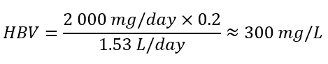
Text description
The health-based value is equal to 2,000 milligrams per day multiplied by 0.2, all divided by 1.53 litres per day. This is roughly equal to 300 milligrams per litre.
Where:
- 2 000 mg/day is the UL established for adults older than 50 years old and is the most conservative UL for individuals 1+ years old (IOM, 2011); there are no data indicating that infants are more sensitive to excess calcium compared to adults.
- 0.20 is the allocation factor for drinking water; it is used as a “floor value,” since drinking water is not a major source of exposure to calcium, and there is evidence of the widespread presence of calcium in one of the other media (such as food) (Krishnan and Carrier, 2013).
- 1.53 L/day is the daily volume of water consumed by an adult (Health Canada, 2021).
3.1.3 Hardness
Hardness is most often measured as the sum of magnesium and calcium present, expressed as equivalent CaCO3, which is the traditional unit of measurement for hardness (see section 1.1.1 Calcium, magnesium, hardness). Thus, an HBV for water hardness can be derived if both magnesium and calcium have proposed HBVs. However, it is not possible to calculate a relevant HBV for magnesium since the UL for magnesium only applies to magnesium from non-food sources such as supplements (see section 3.1.1 Magnesium). Detrimental health effects caused by excess magnesium and/or calcium (that is, the two principal ions that make up water hardness) are generally caused by consumption of supplements rather than food and drinking water. Thus, an HBV for hardness is not warranted.
3.2 Chloride and sulphate
3.2.1 Chloride
To protect against the risk of elevated blood pressure associated with sodium chloride intake, IOM (2005) derived ULs for both sodium and chloride. A UL of 3 600 mg/day for individuals 13+ years old was established for chloride. An HBV can be derived using the reported UL by the IOM (2005) as follows:
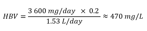
Text description
The health-based value is equal to 3,600 milligrams per day multiplied by 0.2, all divided by 1.53 litres per day. This is roughly equal to 470 milligrams per litre.
Where:
- 3 600 mg/day is the UL for chloride for individuals 13+ years old (IOM, 2005).
- 0.20 is the allocation factor for drinking water; it is used as a “floor value,” since drinking water is not a major source of exposure to calcium, and there is evidence of the widespread presence of calcium in one of the other media (such as food) (Krishnan and Carrier, 2013).
- 1.53 L/day is the daily volume of water consumed by an adult (Health Canada, 2021).
3.2.2 Sulphate
Epidemiological data are insufficient to use as the basis for developing an HBV for sulphate. Although several studies have examined the effects of exposure of humans to sulphate in drinking water, none can be used to derive a dose-response characterization. Peterson (1951), Moore (1952) and Cass (1953) published long-term toxicological data showing a correlation between sulphate consumption and laxative effects. These data are insufficient because they were based on recall with little scientific weight (based on a YES/NO survey) and there were varying levels of magnesium and TDS in the water samples (U.S. EPA, 2003a). The majority of short-term toxicological studies did not find a significant association between sulphate consumption and diarrhea (Esteban et al., 1997; Heizer et al., 1997; U.S. EPA, 1999b). One short-term toxicological study published by Chien et al. (1968) showed a correlation between sulphate consumption and diarrhea in infants. However, the TDS concentration of the drinking water was high (2424 mg/L to 3123 mg/L) and there were limited participants (N = 3).
Adverse effects correlated with ingestion of sulphate were noted in two animal studies. However, neither of these studies is suitable for deriving an HBV. Narotsky et al. (2012) noted dose-related frequency of diarrhea in rats consuming sodium sulphate in drinking water. It was not stated if the frequency of diarrhea was statistically significant between dosage groups, thus the requirements for benchmark dose modelling are not met. In addition, neither a No Observed Adverse Effect Level (NOAEL) or Lowest Observed Adverse Effect Level (LOAEL) can be calculated, since sodium sulphate dosages were given in g/L in drinking water, and body weight and water consumption changed throughout the experiment. Therefore, accurate dosages could not be obtained when converting the provided g/L sodium sulphate dosages to mg/kg bw per day for the HBV calculation. Gomez et al. (1995) noted diarrhea in piglets with ingestion of dietary sulphate ≥ 1,600 mg/L. This study is also not ideal to derive an HBV for reasons similar to Narotsky et al. (2012). IOM has considered this study and concluded it was not suitable to derive a UL (IOM, 2005).
An HBV for sulphate is therefore not proposed. However, multiple international agencies have stated that catharsis/laxative effects and gastrointestinal irritation can occur when drinking water with sulphate levels ≥ 500 mg/L is ingested (NHMRC, NRMMC, 2011; WHO, 2017).
3.3 Total dissolved solids (TDS)
Since TDS is made up of numerous salts, it is challenging to derive an HBV for this parameter. The health effects correlated with specific salts that make up TDS must be analyzed separately. Many salts that make up TDS that may cause adverse health effects (for example, boron, fluoride, nitrate, arsenic and chromium) already have separate established HBVs. Thus, an HBV for TDS is not warranted.
3.4 Hydrogen sulphide
The toxicological data on hydrogen sulphide are insufficient to use as the basis for developing an HBV because all the available studies, except one, are based on inhalation/air exposure of hydrogen sulphide and not oral exposure (Beauchamp et al., 1984; Arnold et al., 1985; Jäppinen and Tola, 1990; Haahtela et al., 1992; Kilburn and Warshaw, 1995; Richardson, 1995; Vanhoorne et al., 1995; Bates et al., 1997, 1998; Hessel et al., 1997; Legator et al., 2001; WHO, 2003; Lewis and Copley, 2015; ATSDR, 2016). Only one oral animal study was found in the literature (Wetterau et al., 1964). There was a 23% decrease in body weight gain at 6.7 mg/kg bw per day in pigs exposed for 104 days and diarrheic digestive disturbances in pigs exposed to 15 mg/kg bw per day for a few days. Interpretation of this study is limited because very few details are reported (for example, no information on methods used, strain used, number of animals studies or statistics) (ATSDR, 2016). Thus, an HBV cannot be derived using animal data. IOM and Health Canada have not derived Recommended Daily Intakes for sulphide. Thus, an HBV cannot be derived using a Recommended Daily Intake such as the UL. An HBV is therefore not proposed for sulphide.
4.0 Analytical considerations
Standardized methods, commercial online analyzers and portable test kits (Table 7) are available for the analysis of calcium, magnesium, hardness, chloride, sulphate, TDS and hydrogen sulphide in source and drinking water. Method detection limits (MDL) are dependent on the sample matrix, instrumentation and selected operating conditions, and will vary between individual laboratories. These methods are subject to a variety of interferences which are outlined in the respective references or instructions.
To accurately measure the concentration of operational parameters using online analyzers and test kits, utilities should develop a quality assurance and quality control program such as those outlined in Standard Methods 3020 (APHA et al., 2018). Periodic verification of results using an accredited laboratory is recommended. Water utilities should check with the responsible drinking water authority to determine whether results from analyzers are acceptable for compliance reporting.
Drinking water utilities should discuss sampling requirements with the accredited laboratory conducting the analysis to ensure that quality control procedures are met and that method reporting limits are low enough to ensure accurate monitoring.
| Parameter | Standardized Method | Online Method | Test KitFootnote * |
|---|---|---|---|
| Calcium | X | X | X |
| Magnesium | X | X | X |
| Hardness | X | X | X |
| Sulphate | X | X | X |
| Chloride | X | X | X |
| TDS | X | X | X |
| Hydrogen sulphide | X | X | X |
|
|||
4.1 Standardized methods
4.1.1 Calcium, magnesium, hardness
Standard methods using atomic absorption spectroscopy and titration can be used for measuring the concentration of calcium and magnesium (Tables 8 and 9). SM 2340B (APHA et al., 2018) is the preferred method for calculating total hardness as the sum of the results from the individual analysis of calcium and magnesium.
| Method (Reference) |
Calcium | Magnesium | Interferences/Comments |
|---|---|---|---|
| EPA 200.5 Rev. 4.2 (U.S. EPA, 2003c) |
X | X | Analytical range not provided. |
| EPA 200.7 Rev. 4.4 (U.S. EPA, 1994) |
X | X | Analytical range not provided. Subject to matrix interference: TDS > 0.2% (w/v). |
| EPA NERL 215.1 (U.S. EPA, 1978a) |
X | N/A | Optimal range 0.2 mg/L to 7.0 mg/L using a wavelength of 422.7 nm. Subject to interference from ionic compounds.pH > 7 will result in lower calcium concentration |
| EPA NERL 242.1 (U.S. EPA, 1978b) |
N/A | X | Optimal range: 0.02 mg/L to 0.5 mg/L using a wavelength of 285.2 nm. Subject to interference from aluminum. Interference from sodium, potassium and calcium at concentration > 400 mg/L. |
| SM 3120B (APHA et al., 2018) |
X | X | Ca upper limit range: 100 mg/L using a wavelength of 317.93 nm. Mg upper limit range: 100 mg/L using a wavelength of 279.08 nm. Subject to interference when TDS > 1 500 mg/L |
| SM 3111B (APHA et al., 2018) |
X | X | Ca optimal range: 0.2 mg/L to 20 mg/L using a wavelength of 422.7 nm. Mg optimal range: 0.2 mg/L to 2.0 mg/L using a wavelength of 285.2 nm. High concentration of phosphate may interfere with the determination of calcium and magnesium; use SM 311D for calcium.. |
| SM 3111D (APHA et al., 2018) |
X | N/A | Ca optimal range: 0.2 mg/L to 20 mg/L using a wavelength of 422.7 nm. Mg optimal range:0.2 mg/L to 2.0 mg/L using a wavelength of 285.2 nm. Subject to interference from phosphate in the determination of magnesium. |
| USGS-NWQL: I-7152 (USGS, 1985a) |
X | N/A | Two analytical ranges: 0.01 mg/L to 5.0 mg/L and 1.0 mg/L to 60 mg/L. Subject to interference from phosphate, sulphate and aluminum. pH above 7 will result in lower calcium concentration. |
| USGS-NWQL: I-4447 (USGS, 1985b) |
N/A | X | Two analytical ranges: 0.01 mg/L to 5.0 mg/L and 2.5 mg/L to 50 mg/L. Subject to interference from aluminum > 2 000 g/L and sodium, potassium and calcium at concentration > 400 mg/L. pH above 7 will result in lower calcium concentration |
|
|||
| Method (Reference) |
Calcium | Hardness | Interferences/Comments |
|---|---|---|---|
| EPA NERL 130.2 (U.S. EPA, 1971a) |
N/A | X | Analytical range not provided. Metal ions may cause fading or indistinct end points. |
| EPA NERL 215.2 (U.S. EPA, 1978c) |
X | N/A | Applicable range: 0.5 mg/L to 25 mg/L as CaCO3. Strontium, magnesium and barium interferences. Alkalinity in excess of 30 mg/L may cause an indistinct end point. |
| SM 3500-Ca B (APHA et al., 2018) |
X | N/A | Analytical range not provided. Subtraction for Mg. Not recommended for sample containing phosphorus > 50 mg/L |
| SM 2340 Hardness C (APHA et al., 2018) |
N/A | X | Analytical range not provided. Some metal ions may cause interference. Determine calcium and magnesium by a non-EDTA method when there is a high level of heavy metals presents. |
| USGS-NWQL: I-3338 (USGS, 1985c) |
N/A | X | Analytical range not provided. Not applicable for acidic water with excessive amount of heavy metals. |
|
|||
4.1.2 Chloride and sulphate
The standardized method for measuring chloride and sulphate uses ion chromatography (Table 10). Turbidimetric, gravimetric and potentiometric standard methods are also available (Tables 11 and 13). SM 4500-Cl- and SM 4500-SO42- can be used to aid in the selection of method for the determination of chloride and sulphate respectively.
| Method (Reference) |
Chloride | Sulphate | Interferences/Comments |
|---|---|---|---|
| U.S. EPA 300.1, Rev. 1.0 (U.S. EPA, 1999c) |
X | X | Analytical range not provided. Low-molecular-weight organic acids, bromate and chlorite may interfere with the determination of chloride and must be purged with an inert gas. |
| SM 4110 B (APHA et al., 2017) |
X | X | Analytical range not provided. Filter particles larger than 0.45µm. Low-molecular-weight organic, acids, bromate and chlorite may interfere with the determination of chloride and must be purged with an inert gas. |
| SM 4110 C (APHA et al., 2017) |
X | X | Analytical range not provided. |
| EPA-NERL: 375.4 (U.S. EPA, 1978d) |
N/A | X | Applicable range: 1 to 40 mg/L. Suspended matter and colour may interfere. |
|
|||
| Method (Reference) |
Chloride | Sulphate | Interferences/Comments |
|---|---|---|---|
| SM 4500- SO42- E (APHA et al., 2017) |
N/A | X | Suitable analytical range: 1mg/L to 40 mg/L. Colour or suspended matter in large amounts will interfere. |
| SM 4500-Cl- B (APHA et al., 2017) |
X | N/A | Suitable analytical range: 0.15 mg/L to 10 mg/L. Sulphide, thiosulphate and sulphite ions interfere. |
| SM 4500-Cl- C (APHA et al., 2017) |
X | N/A | Analytical range not provided. |
|
|||
| Method (Reference) |
Sulphate | Interferences/Comments |
|---|---|---|
| SM 4500-SO42- C (APHA et al., 2017) |
X | Suitable analytical range: > 10 mg/L. Gravimetric determination of SO42- is subject to errors; refer to 4500-SO42-A on the interferences. |
| SM 4500- SO42- D (APHA et al., 2017) |
X | Suitable analytical range: > 10 mg/L. |
| Method (Reference) |
Chloride | Interferences/Comments |
|---|---|---|
| SM 4500-Cl- D (APHA et al., 2017) |
X | Analytical range not provided. |
4.1.3 Total Dissolved Solids (TDS)
Standardized methods are available for measuring TDS. SM 2540 B-D (APHA et al., 2020) is suitable for TDS concentrations ranging from 2.5 mg/L to 200 mg/L. The major ionic constituents of TDS (sodium, calcium, magnesium, chlorides, sulphates, etc.) can also be measured individually and summed to produce an estimate of overall TDS using SM 2510 A 3020 (APHA et al., 2017).
Alternatively, SM 2510 (APHA et al., 2017) and Hach Method 8160 (Hach Co., 2021) considers conductivity as a surrogate measure of total dissolved solids and may be used for rapid quantification and process monitoring capabilities. This method uses a conductivity probe and should only be used if a calibration curve has previously established the correction factor for the specific water type.
4.1.4 Hydrogen sulphide
There are four categories of sulphide in water (total sulphides, dissolved sulphides, acid-volatile sulphide or un-ionized hydrogen sulphide) that can be measured (Table 14 Figure 4500-S2-:1) found in Standard Methods (APHA et al., 2017). This table can be used to aid in the selection of methods for the determination of sulphide under various conditions. SM 4500-S2- H provides guidance calculating un-ionized hydrogen sulphide (APHA et al., 2017).
| Method (References) |
Methodology | Interferences/Comments |
|---|---|---|
| SM 4500-S2- D (APHA et al., 2017) |
Colorimetric | Suitable analytical range: 0.1 mg/L to 20 mg/L. |
| SM 4500-S2- E (APHA et al., 2017) |
Gas Dialysis with Methylene Blue | Suitable analytical range: 0.002 mg/L to 0.100 mg/L. |
| SM 4500-S2- I (APHA et al., 2017) |
Distillation with Methylene Blue | Suitable analytical range: > 1 mg/L. Measures total sulphide, which includes hydrogen sulphide and acid-soluble metal sulphides present in suspended matter. |
| SM 4500-S2- F (APHA et al., 2017) |
Iodometric | Analytical range not provided. |
| SM 4500-S2- G (APHA et al., 2017) |
Ion-selective electrode | Suitable analytical range: > 0.03 mg/L. Humic acid may interfere with silver/sulphide ion-selective electrode. |
| USGS-NWQL: I-3840 (USGS, 1985d) |
Iodometric titration | Suitable analytical range: > 0.5 mg/L. Reducing substances such as sulphites and heavy-metal ions react with iodine. |
4.1.4.1 Sample preservation and preparation for hydrogen sulphide
Ballinger and Lloyd (1981) noted that gentle shaking of the sample for 10 seconds resulted in the loss of 15% of hydrogen sulphide from the solution. Therefore, it is important that samples are collected with minimum agitation and aeration to minimize loss of hydrogen sulphide from solution, and to ensure the analytical results reflect the hydrogen sulphide concentration at the time and point of sample collection.
Sample preservation considerations for the analysis of hydrogen sulphide in drinking water can be found in the references listed in Table 14. SM 4500-S2- C provides guidance on sample pretreatment to remove interfering substances (such as reducing agents) for the methylene blue and iodometric methods (APHA et al., 2017). Zinc acetate is commonly used for preserving the water sample at the time of collection (Goodwin et al., 1998, APHA et al., 2017). It is important to ensure that sample preservation follows the sampling handling procedure stated in the selected method.
4.2 Online analyzers and portable test kits
4.2.1 Calcium, magnesium and hardness
Commercial online and portable analyzers based on conductivity, electrochemical and optical sensing principles are available for quantifying hardness. For monitoring of softening processes, the use of continuous online methods may be appropriate. Semi-batch colorimetric titrations with EDTA can provide process control signal for optimized control of softening processes. Kruse (2018) noted that conductivity methods to measure hardness has its limitation as there are minerals that do not contribute to hardness but contribute to conductivity.
Portable (field) test kits (Table 15) for the analysis of calcium, magnesium and total hardness are also available and suitable for routine monitoring of treatment facilities and distribution systems where rapid results are favoured over analytical accuracy. Calcium, magnesium and hardness are all expected to remain stable throughout a water distribution network. However, field testing may be required for remote locations and to verify the stability of the concentrations throughout the distribution system. Several manufacturers provide colorimetric test kits that can be read with either a visual colour comparator or a portable spectrophotometer.
| Method (Reference) |
Calcium | Magnesium | Total Hardness | Interferences/Comments |
|---|---|---|---|---|
| Hach 8204- Titration with EDTA (Hach, 2019) |
X | N/A | N/A | Orthophosphate causes a slow endpoint. |
| Hach 8030- Calmagite colorimetric (Hach, 2015a) |
X | X | N/A | Range up to 4.0 mg/L as CaCO3. Dilution required above this level. |
Hach 8213- Titration with EDTA |
N/A | N/A | X | Range 10 to 4 000 mg/L as CaCO3. |
|
||||
4.2.2 Chloride and sulphate
Online and portable analyzers are available for quantifying sulphate. Some of these analyzers are based on the colorimetric method (Table 16) titration systems using solid state lead/sulphate-ion-selective electrode. A variety of test kits are available commercially for the detection of chloride and sulphate in drinking water based on mercuric nitrate and turbidimetric methods, respectively.
| Method (Reference) |
Sulphate | Interferences/Comments |
|---|---|---|
| EPA 375.2, Rev. 2.0 (U.S. EPA, 1993b) |
X | N/A |
| EPA-NERL: 375.1 (U.S. EPA, 1971b) |
X | Range: 10 mg/L to 400 mg/L. Cations may interfere. |
| SM 4500-SO42- F (APHA et al., 2017) |
X | N/A |
|
||
4.2.3 Total dissolved solids (TDS)
Commercial online and portable probes based on conductivity are also available for providing quick measurements of TDS in water. Depending on the manufacturer and/or calibration, these portable probes can typically measure TDS levels up to 1 g/L and some can measure as high as 500 g/L.
4.2.4 Hydrogen sulphide
A variety of test kits are available commercially for the detection of hydrogen sulphide in drinking water. Test strips are based on a colorimetric method where the paper will develop a colour when exposed to hydrogen sulphide. This method typically provides a reading within a minute. However, the tests are not as precise as laboratory methods.
Test kits are available and are more precise than test strips. However, some of the test kits require a portable colourimeter or spectrophotometer to determine the hydrogen sulphide concentration. Real-time analyzers are also available to obtain rapid measurement of hydrogen sulphide concentration in drinking water. Pandey et al. (2012) completed a review of the sensor-based method commonly used for monitoring hydrogen sulphide, including comparing the general response time, limit of detection, common operating range and limitations of the different technologies. As with the laboratory methods, it is important that samples that will be tested with kits or strips are collected with minimum agitation and aeration to minimize loss of hydrogen sulphide from solution to ensure the analytical results reflect the hydrogen sulphide concentration at the time and point of sample collection.
5.0 Treatment considerations
5.1 Municipal-scale treatment
Treatment technologies are available for the reduction of all seven operational parameters at the municipal level. Water utilities should balance aesthetic (visual, taste and odour) and health-based considerations and operational concerns (scaling in distribution and plumbing systems and household appliances, fouling of ultraviolet units, corrosion control) with proper removal and disinfection of microorganisms. Measures taken to reduce the parameters in this guideline (calcium, magnesium, hardness, chlorides, sulphates, TDS and hydrogen sulphide) should not compromise the disinfection process. It is also possible that treatment strategies that aim to reduce one parameter could potentially lead to unintended downstream effects.
The selection of an appropriate treatment technology for a specific water supply will depend on many factors, including the characteristics of the raw water supply, the concentration of the parameter and the operational conditions of the specific treatment method. For example, ionic strength of the source water may impact the efficacy of coagulants and jar testing is recommended when using a coagulation process. These factors should be taken into consideration to ensure that the treatment technology selected is capable of reducing the parameters of interest in the drinking water. Since these parameters are considered to have both operational and aesthetic significance for drinking water, it is important to ensure that the consumers find the treated water acceptable for drinking or they may obtain water from unsafe alternative sources.
As these naturally occurring parameters exist in the environment together, the treatment technologies for these parameters are often grouped together in the scientific literature. As such, the reduction of calcium, magnesium, hardness, chloride, sulphate and TDS are discussed in a grouped approach in this guideline document. Due to the offensive odour of hydrogen sulphide, this parameter is often removed to the lowest possible concentration.
Bench- or pilot-scale testing is recommended prior to implementing process changes or introducing a new source to ensure the water can be successfully treated and an optimal process design is established.
5.1.1 Calcium, magnesium and hardness
Total hardness is generally not an aesthetic concern unless it is related to the taste threshold for calcium or magnesium. Treatment technologies available to reduce hardness level include traditional softening, IX and membrane filtration treatment.
Drinking water utilities and private consumers may choose not to treat these aesthetic concerns on the basis that they do not affect the safety of water. Elevated hardness in distribution systems can lead to scale formation or incrustation on pipe walls resulting in frictional pressure losses throughout the distribution system. Hardness-related pipe fouling can be mitigated by reducing hardness levels or by adjusting the pH to increase the solubility of the precipitating ions. Scale formation is particularly noticeable within premise plumbing or on plumbing fixtures as a white powdery or scaly deposit. Deposits within hot water tanks and other heating vessels can impede heat transfer resulting in lower energy efficiencies and premature failure (Hofman et al., 2006). Davis (2010) noted that magnesium levels in excess of approximate 40 mg/L as CaCO3 can form scales in hot water heaters.
In cases where water providers seek to reduce the impact of calcium and magnesium, they often aim to reduce hardness rather than designing for complete removal as soft water can lead to corrosion in drinking water distribution systems and in household plumbing. More information on corrosion control can be found in Health Canada’s Guidance on Sampling and Mitigation Strategies for Controlling Corrosion (Health Canada, 2022a). Hardness can be reduced through chemical precipitation (softening), IX or membrane filtration processes. The selection of removal technologies will depend on the type of hardness (carbonate or non-carbonate) that needs to be reduced.
While calcium and magnesium are often the most prevalent cations in solution, it is important to note the presence of sodium and potassium as they also contribute to the ionic strength of a solution. More information on potassium can be found in the Health Canada drinking water guideline document (Health Canada, 2008).
5.1.1.1 Lime softening
Softening refers to the removal of the multivalent ions that cause hardness. At the municipal scale, this is often accomplished through the chemical precipitation of hardness ions by the addition of hydrated lime (calcium hydroxide Ca(OH)2), soda ash (sodium carbonate Na2CO3) and/or caustic soda (sodium hydroxide NaOH). Quicklime (calcium oxide CaO) is often used and is rehydrated by the addition of water to create a slurry of hydrated lime which is then used for softening (Davis, 2010). The extent of hardness reduction depends on the type of precipitation agent applied, the dosage, the temperature, the pH of a water system and the contact time achieved in the process. Chemical stoichiometry, solution of simultaneous equilibria equations, softening diagrams and appropriate testing (for example, jar tests, pilot test) can be used for determining the appropriate precipitation agent and dosage (Letterman and American Water Works Association, 1999; Davis, 2010; Crittenden et al., 2012). As softening raises the pH level of the water to above 10 and sometimes to as high as 11.5, the process can inactivate some microorganisms as many cannot survive above a pH of 10.5 (Logsdon et al., 1994; AWWA, 1999; 2016).
For source water with high carbonate hardness and low magnesium hardness, single-stage lime softening is the simplest method. Hydrated lime is added to raise the pH of the water to approximately 9.5–10 to precipitate calcium-related hardness (Crittenden et al., 2012). The amount of CaCO3 and Mg(OH)2 precipitation increases with pH up to an equilibrium of 10.3 and 10.8, respectively. However, this pH may vary slightly due to the interactions of calcium and magnesium with other solutes in the water (Letterman and American Water Works Association, 1999). In raising the pH, the bicarbonate ions are converted to non-soluble carbonate ions (Droste, 2019; Letterman and American Water Works Association, 1999). When the source water contains high concentrations of calcium and magnesium, excess lime is used to raise the pH above 11.0 in order to precipitate the magnesium carbonate and magnesium hydroxide along with the calcium (AWWA, 1999; Lawler and Kweon, 2003; Crittenden et al., 2012).
When there are significant levels of magnesium and/or non-carbonate hardness present in the source water, soda ash can be added in a subsequent stage to achieve the desired hardness reduction at a pH greater than 10.5 (Cadena et al., 1974; Crittenden et al., 2012). Caustic soda may also be used to precipitate calcium hardness when there is insufficient carbonate hardness to react with lime (Crittenden et al., 2012). This reaction produces less sludge but is generally more costly compared with the lime softening methods due to the wide availability of lime (Mercer et al., 2005; Davis, 2010).
Generally, the lowest hardness level that can be achieved with the lime softening for calcium is 30 mg/L as CaCO3 and for magnesium, 10 mg/L as CaCO3. This limitation is due to the solubility of CaCO3 and Mg(OH)2, the physical constraint of mixing and contact, and the lack of sufficient time for the reaction to go to completion (Davis, 2010). The theoretical limit for the reduction of hardness in water through the lime-soda ash softening processes is 13.5 mg/L as CaCO3 (Cadena et al., 1974).
If present, natural organic matter (NOM) may also precipitate and slow the precipitation of hardness (Mercer et al., 2005). Carbon dioxide (CO2) and carbonic acid need to be neutralized prior to raising the pH as they will compete to react with the lime before softening can occur (Letterman and American Water Works Association, 1999; AWWA, 2016).
Where the pH has been increased above the CaCO3 saturation point, it is often necessary to recarbonate the water through the addition of CO2. This will stop the precipitation reaction, preventing CaCO3 deposition in the downstream of the treatment process and in the distribution system (Davis, 2010). The addition of CO2 results in the conversion of carbonate into bicarbonate alkalinity and lowers the bulk water pH to a more neutral range (Hill, 1924). Careful control of CO2 is important as it can react with excess lime to form CaCO3 (AWWA, 2016) and increase the hardness level. Post-chlorination (with chlorine gas) may be sufficient to reduce the pH to saturation pH without the need to recarbonate the water (Crittenden et al., 2012).
Contact times for lime-softening are highly dependent on temperature, with longer reaction times required under cold water conditions. Contact times may not be sufficient to achieve a chemical equilibrium state in the chemical mixing plants (Hoover and Langelier, 1938), but rather reach the point at which reactions slow down considerably. Downstream filters will need to be monitored for excess precipitation of hardness solids if the reactions are incomplete in the lime-softening stage of the treatment plant. The detailed effects of each of these conditions (such as contact time, pH, etc.) are discussed in several literature resources (Droste et al., 1997; Crittenden et al., 2012). The chemical equations and process flow diagrams of the softening processes described above are available in Droste et al., 1997; Letterman and American Water Works Association, 1999; Davis, 2010; Crittenden et al., 2012; and AWWA, 2016.
In a study of integrated water treatment of softening and ultrafiltration, it was noted that the characteristics (such as size, structure, surface charge) of the precipitates (for example, CaCO3, Mg(OH)2) formed during the softening process can influence harness removals (Lawler and Kweon, 2003). Randtke et al. (1982) found that when lime is used for softening, the crystals formed are small and settled slowly, leading to high removal of Ca+. When NaOH is used to initiate the process, it produces many nuclei which precipitated quickly, resulting in a higher residual calcium concentration. Soda-induced precipitates resulted in a lower amount of calcite. These properties affect the removal of hardness ions as they affect the settling velocity and chemical affinity for individual compounds (Lawler and Kweon, 2003). The softening process can reduce other parameters in the raw water concurrently. A list of inorganic parameters and their observed removal rate is available (Letterman and American Water Works Association, 1999; Davis, 2010).
5.1.1.2 Blending
Blending or split treatment is a more advanced form of precipitative softening, where the treatment train includes a secondary flow that bypasses the lime-softening basins and is recombined with the completely softened water downstream from the lime-softening basins (Davis, 2010; Crittenden et al., 2012). It was intended as a means of simple and economical process control that required far less operator intervention than a traditional lime-softening plant (Cherry, 1955; Rossum, 1955; Black, 1966). The split stream design allows for reduced operational costs by only treating a portion of the water for hardness removal followed by blending with other water within the treatment plant (Cherry, 1955; Shuey, 1966; Davis, 2010).
This process allows for greater removal of magnesium hardness as the basins can achieve oversaturation and precipitation of both calcium and magnesium in a single step (Zipf et al., 1981). Split treatment with excess lime can reduce magnesium to its solubility limit of 10 mg/L as CaCO3 (Letterman and American Water Works Association, 1999). Soda ash may be added to the recombined stream to reduce non-carbonate hardness (Zipf et al., 1981). The recombined stream may need to be recarbonated through the addition of CO2 gas to achieve stable pH and water quality characteristics. Zipf et al. (1981) noted that recarbonation may not be needed for the lime-soda ash process and or if there is an adequate return of sludge with the recombined water. The authors also developed a methodology for understanding the equilibria relationships to determine the desired effluent concentrations and operating variables that may be useful for plant operators. Attention must be given to the water quality of a new source prior to making any changes (such as switching, blending and interconnecting) to an existing supply. For example, if the new water source is more corrosive, it may cause leaching of lead or copper in the distribution system. The water quality of the recombined stream should be analyzed to ensure it meets the desired levels.
5.1.1.3 Enhanced precipitative softening
Enhanced precipitative softening aims to reduce the levels of hardness as well as dissolved organic carbon (DOC), ultimately reducing the formation of disinfection by-products (U.S. EPA, 1999b; Carlson et al., 2000). Enhanced precipitative softening is typically used for source water with high concentrations of NOM as the precipitated Mg(OH)2 solids could effectively remove the NOM (Lawler and Kweon, 2003). The high lime dosage required for magnesium removal may lead to voluminous sludge and operational problems (Lawler and Kweon, 2003). Rantke et al. (1982) noted that although the DOC reduction had been observed in softening processes, it was unclear what the mechanisms were for this process. They also highlighted the differing effectiveness between softening processes using lime versus soda ash. The presence of multivalent cations (such as Ca2+ and Mg2+) may also cause charge neutralization of negatively charged NOM compounds. However, that is not thought to be the main mechanism of NOM removal in this precipitative softening process. Leentvaar and Rebhun (1982) suggested that much of the total organic carbon removal associated with CaCO3 precipitation was through sweep flocculation, while the removal of magnesium hydroxide was achieved through charge neutralization. Guidance is available on the implementation of enhanced coagulation and precipitative softening (U.S. EPA, 1999b).
5.1.1.4 Filtration
While much of the precipitated solids will settle out in the treatment basins, all softening processes may require a filtration step to remove fine particulate matter. Rapid granular filters are traditionally included in lime-softening plants. However, they may be subject to fouling of the filter media if there is excess particulate carry-over from the lime-softening process. Similarly, membrane elements may also be fouled. In a study of integrated water treatment of softening and ultrafiltration by Lawler and Kweon (2003), it was noted that the degree of pretreatment (such as extent of softening) will influence the degree of fouling and efficacy of the membrane filtration treatment. Due to the kinetics of the softening process, precipitation can continue during settling on the surface or in the pores of the membrane unless the precipitation is chemically stopped. Precipitation occurring on the surface or in the pores will cause the débit to decline. CCPP can be used to control precipitation on the filters. Targets for CCPP after recarbonation are normally less than 5 mg/L entering the filter.
5.1.1.5 IX Softening
IX is a physicochemical process in which there is an exchange of ions in the raw water with ions within the solid phase of a resin (AWWA, 2005; Crittenden et al., 2012). As raw water ions displace ions on the resin, the capacity of the resin is gradually exhausted, resulting in contaminant breakthrough. Once the resin has reached its capacity, the resin must be regenerated to reverse the process. Exchange resins exhibit a degree of selectivity for various ions, depending on ion type and concentration in solution, and the type of resin selected (Davis, 2005; Crittenden et al., 2012). The process is governed by stoichiometric ratios and electroneutrality where the total surface charge of resin beads must be maintained at all times (Crittenden et al., 2012). An exchange resin is initially saturated with monovalent cations (usually sodium) (AWWA, 2005).
Strong acid cation (SAC) exchange resins typically use a strong acid sulphonate group that allows for full dissociation of salts in a water stream (Davis, 2010; Crittenden et al., 2012). Full dissociation of salts allows for the reduction of both carbonate and non-carbonate hardness. This technology is appropriate for a wide pH range and can be regenerated using either a strong acid rinse solution or a sodium salt brine soak (AWWA, 2005; Crittenden et al., 2012). Utilities using SAC resins in the sodium form should be aware that this process may introduce undesirable quantities of sodium in the treated water.
In a bench-scale study conducted in Texas using IX softening (exchange of sodium for Ca and Mg), the system was able to reduce the hardness level from 388 mg/L down to 7 mg/L, the calcium level from 88 mg/L to 1 mg/L and the magnesium level from 41 mg/L to 1 mg/L (AWWA, 2003). The softened water was then blended with other streams to produce a blended product as finished water. The researchers estimated approximately 2.6 tons of salt per million gallons (MG) of blended product was needed for the softening process. The sodium level increased from 110 mg/L in untreated water to 286 mg/L in the softened water.
5.1.1.6 Membrane filtration
Membrane filtration technologies for hardness reduction in drinking water include reverse osmosis (RO) and nanofiltration (NF) (U.S. EPA, 1999; Odell, 2010). RO membranes can reduce TDS and monovalent ions while NF membranes are mainly used for the reduction of hardness (Ca2+, Mg2+) (Bergman et al,. 1995). RO treatment systems typically require prefiltration for particle removal and often include other pretreatment steps, such as the addition of anti-scaling agents and dechlorination. The membrane permeate has a low pH and is very corrosive due to the acid pretreatment preventing scaling (Davis, 2010). Lime softening followed by filtration and pH adjustment is an effective pretreatment to improve the performance of the RO membrane for enhanced reduction of mineral salt scaling from water sources.
Pretreatment is required to preserve membrane life because the presence of chlorine residuals, particulates, NOM and scale-forming ions (Ca2+, Ba2+, iron and silica) in the feed water can adversely affect the performance of RO membrane technologies. Site-specific testing is recommended to determine the design criteria, potential fouling and pretreatment needs when utilities consider RO membranes. As membrane filtration technologies such as NF and RO can remove a high concentration of bivalent cations (Ca2+ and Mg2+), the permeate is sometimes blended with the feed water to achieve acceptable levels of hardness.
Post-treatment for RO permeate (finished water) typically includes pH adjustment, addition of corrosion inhibitors and disinfection. RO concentrate disposal must also be considered in the design and operation of RO membrane plants. Inorganic scale formation from the precipitation of salts within the membrane module leads to permeate débit decline and shortening of the membrane life. Additional information on CaCO3 scale control can be found in AWWA (2005).
In a pilot-scale study conducted in Texas using RO membranes (pressure at 130 psi, recovery at 81%), hardness was reduced from 388 mg/L down to 3 mg/L, calcium was reduced from 88 mg/L to <1 mg/L and magnesium was reduced from 41 mg/L to <1 mg/L (AWWA, 2003). The RO permeate (68%) was then blended with untreated groundwater (38%) to produce a blended water with hardness at 149 mg /L, calcium at 34 mg/L and magnesium at 16 mg/L. The RO membrane filtration was also able to reduce the TDS level from 702 mg/L down to 14 mg/L in the permeate. The permeate pH was considerably lower than the feed water as acid was added to the feed water to increase recovery. Remineralization with lime, CO2 and sodium bicarbonate is generally needed to reduce the corrosivity of water. Since low mineral content water can leave a bitter, dry or rough taste, remineralization may improve the aesthetic quality of the finished water (Vingerhoeds et al., 2016; Biyoune et al., 2017; Lesimple et al., 2020).
NF membrane filtration can achieve upwards of 98% rejection of magnesium sulphate. NF membranes have much tighter pore sizes (molecular weight cut-off of 500) and reject many larger ions (Conlon and McClellan, 1989). In a pilot study of two commercial membranes using a mix of distilled water with groundwater, the NF membranes achieved a rejection rate between 79.5% and 98.4% for calcium, 83.3% and 99% for magnesium, and 37.8% and 83.4% for hardness (Nasr et al., 2013).
Mulford et al. (1999) completed an NF membrane filtration study at full and pilot scale in Florida with different treatment train set-ups. In this study, the full-scale plant was able to reduce hardness from 290–320 mg/L down to 28–46 mg/L, achieving > 84% reduction in hardness. In a full-scale study at two drinking water treatment plants in Florida, the NF membrane filtration was able to reduce hardness levels from around 250 mg/L down to the range of 10 to 20 mg/L; this water was blended with that from the lime softening process to produce finished water that met quality requirements (Bartels and Wilf, 2007). The authors found that the NF membrane greatly reduced total organic carbon in the finished water compared with lime softening. Tang et al. (2019) evaluated NF membranes for a full-scale water treatment plant in the Netherlands and found that NF membrane filtration was able to reduce hardness levels from 200 mg/L to 130 mg/L, noting that target hardness is achieved by blending non-softened bypass water with softened permeate water.
In a pilot-scale study conducted in Germany, Gorenflo et al. (2002) found that water with a high concentration of sulphate and potentially the complexation of Ca2+ with humic acids resulted in the NF membrane rejecting Ca2+ and Mg2+ at rates that were higher than the manufacturer’s data. The rejection rate for calcium was > 74% and magnesium was > 86%, whereas the concentration of calcium was 114.7 mg/L, magnesium was 12.3 mg/L and sulphate was 99 mg/L in the raw water.
Several bench-scale studies have shown that NF membrane filtration is capable of reducing hardness. Van de Bruggen et al. (2001) studied four types of NF membranes and, depending on the membrane, the hardness level was reduced from 280 mg/L down to between 14 mg/L and 140 mg/L. The authors noted the NF membranes with higher rejection rates were due to pore size and charge effects and interactions of Ca2+ and Mg2+ with membranes that had a positive charge surface. Ghizellaoui et al. (2005) studied the impact of pressure on NF membranes for a very hard water (600 ppm) and found that higher pressure (4–16 bar) resulted in higher retention rates of calcium and bicarbonates (50% and 40%, respectively), while lower pressure (1 and 2 bar) resulted in lower retention rates (34% and 30%, respectively).
5.1.2 Chloride and sulphate
Chloride and sulphate ions are difficult to remove in most water treatment processes. High salt content source waters (such as brackish or marine-influenced aquifers) may require treatment to reduce customer complaints and to achieve a chemically stable water that will not be corrosive for distribution systems and internal building plumbing.
Reductions in chloride and sulphate concentrations can be achieved through anion exchange or RO. Both technologies also have waste streams (concentrated brine) that require further handling to mitigate environmental concerns (U.S. EPA, 1999b).
5.1.2.1 Membrane filtration
RO is capable of > 90% rejection of chlorides and > 69% of sulphates, depending on the membrane unit implemented (Biesheuvel et al., 2019). The specific ionic composition, pH and temperature of the influent stream can have an impact on the overall efficacy of a particular membrane unit. In some cases, a membrane will preferentially remove greater concentrations of the sulphate form of specific salts (sodium sulphate > sodium chloride) due to size differences between the ions of concern.
NF units generally have poor rejection of small monovalent anions such as chlorides (as low as 7%) and are often better suited for the removal of larger multivalent anions such as sulphates (removal > 90%) as shown in a pilot study by Nasr et al. (2013).
A pilot-scale study of an ultrafiltration treatment plant in the Netherlands found that the sulphate concentration was reduced from 140 mg/L to 0.1 mg/L (Duranceau, 2001).
In an NF bench-scale study, Schaep et al. (1998) observed the influence of temperature on the rejection rate of chloride. The rejection was approximately 10% lower at 30 oC (approximately 60% as read from graph) compared with 10 oC (approximately 70%). This may be due to the temperature influencing the viscosity of the water, which impacts the flux. The same was not observed for calcium, magnesium or sulphate in the same study.
RO technology is used primarily to remove inorganic contaminants, and some utilities may choose to blend the treated water with raw water to achieve a non-corrosive product water. In many cases the water produced by RO treatment units is considered corrosive towards distribution systems and household plumbing. Additional treatment may be required to remineralize water prior to distribution. In all cases, system operators must ensure that all microbial treatment requirements are being met prior to delivering water to consumers.
Inorganic scale formation (for example, silica, barium sulphate and CaCO3) remains a serious impediment to achieving high RO recovery and leads to permeate flux decline and shorter membrane life. Lime softening followed by filtration and pH adjustment is an effective pretreatment to improve the performance of RO for enhanced reduction of mineral salt scaling from water sources. Additional information on sulphate scale control can be found in AWWA (2005).
5.1.2.2 Anion exchange
Although anion exchange technology is capable of reducing sulphate, most systems will increase the concentration of chlorides in the discharge. Thus, anion exchange is rarely implemented in municipal drinking water systems for this purpose. Some systems may practice anion exchange for the reduction of nitrate concentrations which will lead to increased chloride levels. Therefore, chloride levels should be monitored when using anion exchange to evaluate if they meet the proposed HBV. Alternative regenerants for IX that do not contain chloride are also available, but may increase the cost of operation.
5.1.2.3 Treatment chemicals
Many inorganic coagulants are chloride- or sulphate-based salts such as aluminum sulphate, ferric sulphate, polyaluminum sulphate, polyaluminum chloride or high-polyaluminum chlorosulphate coagulants (Wu et al., 2020). These coagulants all contribute soluble chlorides and sulphates and may contribute to a large portion of the total of the treated water for conventional coagulation and filtration plants. Direct filtration plants will see a more moderate impact from the chlorides and sulphates during associated coagulation. Disinfection with chlorine gas yields free chloride ions when the aqueous chlorine dissociates to form hypochlorous acid. IX units will also lead to the addition of chlorides as they typically use sodium chloride or potassium chloride as regeneration brines for the IX. While the sodium and/or potassium ions are active in the regeneration exchange reactions, the chloride ions are simply discharged to the waste stream when regeneration is complete. This additional loading of chlorides on the environment is a concern both in local discharge to weeping fields or discharge to the sanitary sewers. Storage or concentration of this brine may be required in order to limit the downstream impacts on the environment. In all applications, it is important to ensure that all treatment chemical used are certified according to NSF/ANSI/CAN Standards 60: Drinking Water Treatment Chemicals – Health Effects (NSF/ANSI, 2021).
5.1.3 Total dissolved solids (TDS)
RO and NF membranes are capable of reducing TDS (AWWA, 2005). Switching between water sources with significantly different TDS on a seasonal basis may be detectable for some consumers and cause undue concerns regarding water quality.
5.1.3.1 Membrane filtration
RO membranes can be used to reduce TDS and monovalent ions (Bergman et al., 1995). RO treatment systems typically require prefiltration for particle removal and often include other pretreatment steps, such as the addition of anti-scaling agents and dechlorination. Pre-treatment for hardness reduction may be required to prevent scaling on the membrane elements. Lime softening followed by filtration and pH adjustment is an effective pretreatment to improve the performance of RO for enhanced reduction of mineral salt scaling from water sources.
NF membranes were capable of reducing some dissolved ions by size exclusion in full-scale treatment plants in Florida, achieving a 33%–75% reduction of TDS (Bergman, 1995). Saitua et al. (2011) found 53% removal of TDS through a pilot-scale membrane filtration using a polyamide membrane treating water with an influent TDS concentration of 1 290 mg/L. In general, larger multivalent ions such as those that cause hardness will be removed through NF membrane filtration. However, monovalent ions will still pass through.
5.1.3.2 IX
Total dissolved solids are often not significantly impacted by IX systems as this technology is designed to exchange hardness ions for non-hardness ions (Crittenden et al., 2012). Davis (2010) noted that strong base anion exchange (SBA) is capable of reducing TDS when the concentration is below 500 mg/L and the sulphate concentration is < 50 mg/L.
Lime softening is capable of reducing TDS through the removal of calcium and magnesium bicarbonates as CaCO3 and Mg(OH)2 solids, respectively. It is important to note that it will also be removing alkalinity and may require additional treatment to address corrosion issues (Clifford, 1999).
5.1.4 Hydrogen sulphide
Hydrogen sulphide is predominantly an issue due to its offensive odour and low odour threshold. Treatment technologies able to remove hydrogen sulphide to 0.05 mg/L include oxidation, aeration and adsorption (Levine et al., 2004a; Crittenden et al., 2012; Lemley et al., 1999; Duranceau et al., 2010; Odell, 2010).
5.1.4.1 Oxidation
Oxidants for hydrogen sulphide control include chlorine, hydrogen peroxide (H2O2), potassium permanganate (KMnO4) and ozone (O3) (Thompson et al., 1995; Levine et al., 2004a; Crittenden et al., 2012). A summarized comparison of different oxidation and the dosage requirements is found in Table 17. A list of their advantages and disadvantages can be found in Duranceau et al. (2010).
| Oxidant | Oxidation reaction | Dose (mg/mg H2S) |
|---|---|---|
| Chlorine | H2S + Cl2 → S0 + 2HCl | 2.08 |
| H2S + 4H2O + 4Cl2 → H2SO4 + 8HCl | 8.33 | |
| Ferrate | 4H2S + 3HFeO4- + 7H+ → 3Fe+2 + S2O3-2 + 2S0 + 9H2O | 2.66 |
| 16H2S + 20HFeO4- + 10H2O → 20Fe(OH)3 + 3H2S2 + SO3-2 + 3S2O3-2 + 3SO4-2 + 6OH- | 4.44 | |
| Hydrogen peroxide | H2S + H2O2 → S0 + 2H2O | 1.03 |
| HS- + 4H2O2 → SO4- 2 + 4H2O + H+ (pH > 8) | 4.11 | |
| Ozone | S-2 + 4O3 + 4H2O → SO4-2 + 4O2 | 5.64 |
| Potassium permanganate | 3H2S + 2KMnO4 → 3S0 + 2MnO22KOH + 2H2O | 3.09 |
| 3S-2 + 8KMnO4 + 4H2O → 8MnO2 + 3SO4-2 + 8KOH | 12.39 |
Chemical requirements for complete sulphide oxidation depend on the solution pH and temperature. Generally, the oxidant dose increases with increasing pH (Cadena and Peters, 1988). Typically, a higher oxidant dose will form sulphate rather than elemental sulphur, resulting in increased turbidity (Cadena and Peters, 1988; Thompson et al., 1995; Levine et al., 2004a).
Crittenden et al. (2012) noted the potential formation of polysulphides when using oxidation to remove hydrogen sulphide. The formation of polysulphides occurs when the hydrogen sulphide concentration is > 1 mg/L and pH < 9. Conversion to sulphate requires an oxidant dose in excess of the stoichiometric requirements and a pH > 8. Polysulphides are difficult to remove, have unique taste and odour, and can complex with metals in distribution systems leading to the formation of black water.
Oxidation of hydrogen sulphide with hydrogen peroxide requires long contact times and large doses of oxidants. This subsequently results in the formation of not only sulphate but also colloidal sulphur, which can increase turbidity in the water (Duranceau et al., 2010; Thompson et al.,1995).
Levine et al. (2004a) conducted a pilot study using hydrogen peroxide coupled with filtration to oxidize groundwater from a wellfield in Florida. The pilot study showed that hydrogen peroxide resulted in > 60% removal at 6.5 minutes of contact time. The tandem use of oxidation catalyzed by ferric sulphate to coagulate the colloidal sulphur showed an increase in hydrogen sulphide removal to > 80% with a shorter contact time (< 6 minutes). The authors concluded that the use of hydrogen peroxide catalyzed by ferric sulphate, coupled with filtration, was capable of reducing hydrogen sulphide (removal data not provided) and produced low turbidity water.
Continuous chlorination is a common method for oxidizing hydrogen sulphide using a dose of 2.0 mg/L for every 1.0 mg/L of hydrogen sulphide (Odell, 2010). In a field study by Lyn and Taylor (1992), chlorine oxidation resulted in the formation of colloidal sulphur at pH > 3.8 and that increasing pH resulted in increased turbidity. The authors also found that aerobic conditions at low pH favoured sulphate formation whereas anaerobic conditions at high pH favoured elemental sulphur formation. The use of chlorine for sulphide oxidation can result in the formation of disinfection by-products (DBPs) such as trihalomethanes and haloacetic acids (Levine et al., 2004a; Thompson et al., 2010; Levine et al., 2006; Stefen et al., 2018).
Ortenberg et al. (2000) found that oxidizing hydrogen sulphide with chlorine was able to completely remove hydrogen sulphide but an objectionable taste was still present. They postulated that the oxidation of hydrogen sulphide with chlorine produced elemental sulphur and polysulphides (H2Sn), which in turn hydrolyzed back into hydrogen sulphide. Stefen et al. (2018) noted that a higher contact time is needed to increase the efficacy of chlorine. However, it can also result in the formation of trihalomethanes.
The use of chlorine dioxide to oxidize hydrogen sulphide resulted in the DBPs chlorite and chlorate, presumably due to the presence of inorganic constituents in the reduced form (Ortenberg et al., 2000). The removal of hydrogen sulphide using ozone was capable of producing sulphate and did not result in any trihalomethanes (Stefen et al., 2018).
Duranceau et al. (2010) noted that using oxygen can result in incomplete oxidation, creating colloidal sulphur and polysulphides. The authors also found that using ferrate as an oxidant reduced sulphide to below the MDL (< 0.3 mg/L). However, the turbidity level increased significantly after contact with this oxidant.
Hydrogen sulphide can be removed from water with potassium permanganate pretreated with sulphuric acid to reduce pH followed by a degasser (Willey et al., 1964). The kinetics for potassium permanganate are rapid with chemical equilibrium occurring 5 minutes after the addition of the oxidant (Cadena and Peters, 1988). The reaction produces floc particles of MnO2 and elemental sulphur, which can be removed by filtration (Duranceau et al., 2010; Edwards et al., 2011). Careful control of the potassium permanganate dose is necessary to prevent the generation of pink water due to excess manganese (Levine et al., 2004a). In addition, the manganese dioxide formed by the reaction can produce excess turbidity in the distribution system (Levine et al., 2004a).
Pilot-scale studies by Duranceau et al. (2010) used hypochlorite as an oxidant for Florida groundwater. The oxidant was used before a proprietary filtration process or a manganese green sand filter. The process was continuously regenerated with bleach to remove hydrogen sulphide from the groundwater. Preliminary results showed that the combination of these technologies was able to reduce sulphides from between 1.4 and 2.6 mg/L to below 1.0 mg/L (detection limit). Another pilot study (Duranceau and Trupiano, 2011) using Florida groundwater evaluated two different oxidized media filtration processes: NaOCl oxidation preceding a proprietary filtration, and NaOCl preceding MnO2 filtration. Both processes were able to reduce sulphide to below detection level (< 0.1 mg/L) and produce finished water with turbidity levels < 1.0 nephelometric turbidity unit (NTU).
5.1.4.2 Aeration
Aeration brings water and air in close contact in order to remove dissolved gases (such as CO2) and oxidize dissolved metals such as iron, hydrogen sulphide and volatile organic compounds. Aeration is a common method for treating sulphides when the concentration is below 2.0 mg/L and when present in the gas phase (Lemley et al., 1999; Duranceau et al., 2010; Odell, 2010). Pre-oxidation is not recommended with aeration of hydrogen sulphide as it may produce sulphide, bisulphide or solid sulphur, which are not air-strippable and would subsequently need to be filtered from the treated water (Odell, 2010).
The pH of water plays a significant role in the form of hydrogen sulphide present. It is difficult to remove hydrogen sulphide in water with a pH > 7 since most of the hydrogen sulphide is present in the forms of HS- and H+ ions. Decreasing the pH of the water entering an aeration system can improve hydrogen sulphide removal efficacy and lower turbidity levels but may result in the formation of some DBPs and increase the copper corrosion rate (Thompson et al., 1995; Edwards et al., 2011). The removal of sulphides at a pH of 6 is roughly 80% and at a pH of 7 is only 70%. (Lemley et al., 1999; Odell, 2010). As water is aerated, CO2 is released, increasing the pH as hydrogen sulphide is converted to HS- thereby reducing the overall efficacy of the stripping process (Levine et al., 2004b; Munter and Vilu, 2008; Crittenden et al., 2012).
Cascade or tray aeration and volatilization in ground storage facilities are only partially effective for sulphide removal which is dependent on pH and atmospheric conditions (for example, more sulphides are removed on windy, warm days) (Duranceau et al., 2010). Montgomery (1985) reported using a cascade tray aerator on the top of a groundwater storage tank and found a removal of only 20% of hydrogen sulphide at ambient pH and temperature. The remaining sulphide was oxidized by chlorine to elemental sulphur in the storage tank. The author noted that the process produced high levels of turbidity and an offensive rotten egg odour.
Packed towers have higher stripping efficacies but CO2 is released faster than hydrogen sulphide. As a result, the pH changes as the water flows down the packing, impacting the removal efficacy (Duranceau et al., 2010). The use of carbonic acid for pH adjustment prior to packed tower aeration can be an effective pretreatment and can also aid in corrosion control (Duranceau et al., 2010).
Aeration technology is widely applied in Estonia through the contact of a thin descending film of water with air on the surface of wood, ceramic or plastic packing. Munter et al. (1999) noted that the sulphide concentration was reduced to 0.3 mg/L from concentrations ranging from an average value of 0.003–0.5 mg/L). A full-scale study on the western coast of Estonia involving groundwater treated by aeration followed by filtration with manganese greensand was able to reduce hydrogen sulphide from a range of 0.64 to 3.4 mg/L down to 0.04 to 0.89 mg/L.
A full-scale trickling filter was able to remove hydrogen sulphide from well water in Greece (Terkerlekopoulou et al., 2010). Water from the two wells was stored in an elevated water tower at 15 m above ground. The water cascaded into the homogenization tank and water aeration occurred through the filter, leading to an elimination of hydrogen sulphide (raw water concentration between 1 and 1.3 mg/L) at the filter outlet (effluent data were not provided).
5.1.4.3 IX
Hydrogen sulphide can be removed using anion-exchange resins since a significant amount of hydrogen sulphide present in water is in ionized form. The effectiveness of the system depends on the resin selected and the concentration of competing anions (sulphate, total organic carbon, and alkalinity) as well as the pH of the water. Typically, chloride resin is used for hydrogen sulphide removal (Lemley et al., 1999; Odell, 2010). The resin can also foul because of the growth of sulphur-related bacteria, which can affect removal efficacy (Duranceau et al., 2010).
Packed-bed anion exchange was capable of removing an influent concentration of 0.82–3.22 mg/L sulphide during a pilot study in Florida (Levine et al., 2006). The removal and effluent data were not provided. The authors also examined the biological enhancements of the anion exchange as the low concentration of dissolved oxygen (< 2 mg/L) promoted the growth of sulphur oxidizing bacteria at the upper surface of the resin, improving the removal of hydrogen sulphide by converting it to either elemental sulphur or sulphate. The by-products of the biological sulphur oxidation, sulphate and elemental sulphur, were removed through the anion exchange. The authors noted the benefits of coupling biological sulphur oxidation with anion exchange increased the exchange capacity, resulting in about two- to three-fold longer operating cycles, thus decreasing the frequency of regenerating the column.
In a pilot plant study by Vidović et al. (2010) using IX followed by an adsorption column, it was shown that up to 60% of hydrogen sulphide in an acid medium (pH 6.6–7.2) can be removed by an IX column and that there is no removal in alkaline medium. The hydrogen sulphide that was not fully removed by the IX was subsequently removed by adsorption.
5.1.4.4 Adsorptive media
Granular activated carbon (GAC) can generally remove hydrogen sulphide to concentrations below 0.3 mg/L (Lemley, 1999; Odell, 2010). Catalytic carbon, a type of activated carbon with a modified surface, has the ability to promote or catalyze chemical reactions. Catalytic carbon can adsorb sulphides onto the carbon surface and, in the presence of dissolved oxygen, it oxidizes the sulphides into elemental sulphur (S8) and sulphate (Megonnell and Spotts, 1994). A minimum dissolved oxygen of 4.0 mg/L is necessary for complete oxidation of hydrogen sulphide into elemental sulphur, which can then be filtered (Saunders and Urbans, 1995; Lemley et al., 1999; Odell, 2010).
A series of pilot-scale studies were performed by Ikehata et al. (2015) in the City of Huntington Beach, California, using coconut shell GAC media (certified to NSF 61) to remove hydrogen sulphide. Using five GAC filters in series, the hydrogen sulphide concentration was reduced from 0.02 and 0.7 mg/L to below MDL of 0.01 mg/L.
Manganese greensand filtration can be used to treat water containing less than 5.0 mg/L of hydrogen sulphide (performance data were not provided). The manganese dioxide coating on the filter catalyzes hydrogen sulphide gas to solid sulphur which is then filtered (Odell, 2010). Willey et al. (1964) conducted a full-sale study at a water treatment plant in central Indiana. The plant had been operating for 2 years and showed that hydrogen sulphide can be removed from water using a regeneration process consisting of a continuous feed of potassium permanganate to the influent of a manganese greensand filter. The authors also concluded that a dilute sulphuric acid feed and aeration eliminated a considerable portion of the hydrogen sulphide (from 11.3 ppm to below MDL) mechanically to reduce the demand for potassium permanganate. Saunders and Lee (1996) noted that when potassium permanganate is used with manganese greensand, the greensand media may become fouled by iron and other contaminants, allowing sulphur to break through if the process runs out of potassium permanganate. Thus, it is important to monitor the manganese greensand filter to ensure it is working optimally.
5.1.4.5 Microbiological filtration
Bacteria can oxidize sulphide into sulphur under oxygen-limited conditions. When dissolved oxygen < 0.1 mg/L, the dominant product is elemental sulphur, while at high levels of dissolved oxygen the dominant product is sulphate (Janssen et al., 1998). Microbiological filtration is capable of reducing hydrogen sulphide but the organisms can slough off surfaces and cause turbidity downstream of storage facilities (Duranceau et al., 2010).
Levine et al. (2004b) conducted pilot-scale studies to compare an inline hydrogen peroxide oxidation coupled with a two stage upflow filtration system with and without the addition of a low dosage of ferric sulphate as catalyzer for the removal of hydrogen sulphide. The addition of ferric sulphate increased the removal of hydrogen sulphide from 20% to 40% (contact time of approximately 2 to 6 minutes) to over 80% (contact time of 2 mins) as well as reduced producing water with turbidity below 0.1 NTU while reducing chlorine demand. This process was capable of reducing hydrogen sulphide and associated turbidity while reducing chlorine demand.
5.1.5 Residuals
Sludge resulting from the addition of lime and/or soda ash can be a major operational burden for utilities that operate chemical precipitation processes (AWWA, 1981). Water utilities should make accommodations to remove these solids on a regular basis, to avoid entrainment of these fine particles in the finished water. It is also possible to reduce the quantities of sludge by partially substituting caustic soda in place of either lime or soda ash.
5.2 Residential-scale treatment
Several treatment technologies can effectively reduce these substances at a residential scale, for example, a small system or household whose drinking water supply is from a private well.
Before a treatment unit is installed, the water should be tested to determine the general water chemistry and the concentration of the parameters of interest found in the source water. Periodic testing by an accredited laboratory should be conducted on both the water entering the treatment unit and the treated water to verify that the treatment unit is effective. Units can lose removal capacity through use and time and need to be maintained and/or replaced. Consumers should verify the expected longevity of the components in the treatment unit according to the manufacturer’s recommendations and service it when required. Systems classified as residential scale may have a rated capacity to treat volumes greater than that needed for a single residence, so they may also be used in small systems.
Certified residential treatment units are available for the reduction of hardness, sulphate, chloride, TDS and hydrogen sulphide.
5.2.1 Calcium, magnesium, hardness
A number of certified residential treatment devices are currently available for the removal of calcium, magnesium or other hardness-contributing elements in drinking water from drinking water. These devices rely on cation exchange, RO and distillation systems.
An IX (water softening) system certified to NSF/ANSI Standard 44 (Residential Cation Exchange Water Softeners) can reduce hardness in drinking water. To be certified for hardness reduction under Standard 44, the device must be capable of reducing hardness to below 1.0 gpg (17.1 mg/L) from an influent hardness of 20 gpg (342 mg/L) (NSF/ANSI, 2022a). Higher concentrations of hardness will require greater amounts of salt to achieve an acceptable level of hardness.
Homeowners with private wells using IX softeners in sodium form should be aware that the treatment unit may introduce undesirable quantities of sodium in the treated water. It is recommended that a separate supply be used for potable water consumption and culinary purposes. When a water softener is used, it is recommended that a portion of the water most frequently consumed (such as kitchen tap) bypass the softener altogether to avoid excessive salt intake. Appendix E contains information on the intake of sodium as a result of water softener use, by hardness level.
An RO system should be able to remove hardness but there are no certified systems available. Additionally, the use of an RO system for removal of high concentrations of hardness would foul the membrane more quickly and require more frequent maintenance as well as shorten the service life of the RO membrane. Consumers may need to pretreat the influent water to reduce fouling and extend the service life of the RO membrane. RO systems are generally not practical for residential-scale point-of-entry (POE) systems as larger quantities of influent water are needed to obtain the required volume of treated water.
The distillation process should also be able to remove hardness but there are no certified systems available. A distillation system certified to NSF/ANSI Standard 62 (Drinking Water Distillation Systems) includes reduction of TDS using sodium chloride as a surrogate. To be certified for TDS reduction under Standard 62, a device must be capable of reducing an average influent concentration of 1 000 mg/L with a minimum reduction of 97% (30 mg/L) (NSF/ANSI, 2022b).
RO and distillation systems are only intended to be installed at point-of-use (POU), as the treated water may be corrosive to internal plumbing components.
A detailed report prepared by Brodeur and Barbeau (2015) using the data from Barbeau et al. (2011) studied the effectiveness of treatment technologies for the removal of manganese in groundwater. This report also included results for hardness removal for 96 systems using various technologies at an average influent concentration of 136 356 µg/L (136.36 mg/L) and treated water concentration of 49 549 µg/L (49.50 mg/L). The authors found that the IX and RO systems were capable of reducing hardness with median removals of 99% and 72%, respectively. Results from the individual technologies are summarized in Appendix D (Table D.1).
5.2.2 Chloride, sulphate
The technologies available for the reduction of chlorides and sulphates at a residential scale are limited. Both chlorides and sulphates tend to remain in solution and are not involved in many chemical reactions. Reductions in the concentrations of chlorides and sulphates may be achieved through anion exchange or RO. A number of certified residential treatment devices are currently available for the removal of chloride and sulphate from drinking water. These devices rely on POU/POE filtration systems.
Distillation systems for sulphate and chloride removal must be capable of reducing an average influent concentration of 800 mg/L to a maximum concentration of 250 mg/L (NSF/ANSI, 2022b).
Homeowners may opt to seek out water sources and aquifers with lower concentrations of these parameters if they find their existing levels are too high.
5.2.3 Total dissolved solids (TDS)
A number of certified residential treatment devices are currently available for the removal of TDS from drinking water. These devices rely on POU/POE filtration systems, RO and distillation systems.
Reduction requirements for TDS are included under NSF/ANSI Standard 42 (Drinking Water Treatment Units – Aesthetic Effects). For a device to be certified for TDS removal under Standard 42, it must be capable of reducing an average influent concentration of 1 500 mg/L to a maximum treated water concentration of 500 mg/L (NSF/ANSI, 2022c).
Reduction requirements for TDS are included under NSF/ANSI Standard 58 (Reverse Osmosis Drinking Water Treatment Systems). For a device to be certified for TDS removal under Standard 58, it must be capable of reducing an average influent concentration of 750 mg/L by at least 75% (down to 187 mg/L) (NSF/ANSI, 2022d).
NSF/ANSI Standard 62 (Drinking Water Distillation Systems) is applicable to the reduction of TDS as sodium chloride in drinking water. For a device to be certified for TDS removal under Standard 62, it must be capable of reducing an average influent concentration of 1 000 mg/L with a minimum reduction of 97% (30 mg/L) (NSF/ANSI, 2022b).
Water that has been treated using RO or distillation may be corrosive to internal plumbing components. Therefore, these units should be installed only at the POU. As large quantities of influent water are needed to obtain the required volume of treated water, RO systems are generally not practical for POE installation. A consumer may need to pretreat the influent water to reduce fouling and extend the service life of the RO membrane.
5.2.4 Hydrogen sulphide
Certified residential treatment devices are currently available for the removal of hydrogen sulphide from drinking water. These devices rely on POU/POE filtration systems. Reduction requirements for hydrogen sulphide are included under NSF/ANSI Standard 42 (Drinking Water Treatment Units –Aesthetic Effects). For a device to be certified for hydrogen sulphide removal under Standard 42, it must be capable of reducing an average influent concentration of 1.0 mg/L to a maximum permissible product water concentration of 0.05 mg/L (NSF/ANSI, 2022c).
6.0 Management strategies
All water utilities should implement a risk management approach such as the source-to-tap or water safety plan approach to ensure water safety. These approaches require a system assessment to characterize the source water, describe the treatment barriers that prevent or reduce contamination, identify the conditions that can result in contamination and implement control measures. Operational monitoring is then established and operational and /management protocols such as are instituted (for example, standard operating procedures, corrective actions and incident responses are instituted). Other protocols are also implemented (such as record keeping and consumer satisfaction) to validate the water safety plan, such as record keeping and consumer satisfaction are also implemented. Operator training is also required to ensure the effectiveness of the water safety plan at all times (Smeets et al., 2009).
Management strategies to reduce concentrations of operational parameters in drinking water may be achieved by:
- Adopting centralized treatment for parameter(s) of concern while considering downstream effects on distribution systems.
- Considering blending source waters with lower concentrations of these parameters.
- Reviewing source water characteristics and the concentration of parameter(s) of concern, and possibly adopting a new source with lower concentrations.
- Addressing any anthropogenic sources of the parameters of concern.
- Providing public information on the appropriateness of POE or POU systems for individual consumers.
6.1 Control strategies
In water sources with higher than acceptable concentrations of operational parameters, one or more treatment options (see section 5.0) may be implemented. Other control strategies may include controlled blending prior to system entry-point, interconnecting with and/or purchasing water from another water system, or use of alternative water supplies. Attention must be given to the water quality of a new source prior to making any changes (such as switching, blending and interconnecting) to an existing supply. For example, if the new water source is more corrosive, it may cause leaching of lead or copper in the distribution system. The water quality of the recombined stream should be analyzed to ensure it meets the desired concentrations.
6.1.1 Blending
A common practice in water softening is bypass blending, which involves diverting a portion of the influent flow around the treatment vessel and blending the diverted water with the treated water. Blending of finished water with raw water may stabilize finished water and decrease the cost of treatment by reducing the volume of water treated. This can result in less frequent regeneration and a savings in chemical and brine disposal costs (U.S. EPA, 1999b). However, the concentration of each parameter in the bypass water needs to be considered to ensure that the finished water concentration does not exceed the treatment objectives.
Utilities implementing control options that involve a new, blended or interconnected source of water for addressing the hardness concentration should assess the water quality of new sources and blended water to ensure that it does not interfere with the existing treatment processes, impact the distribution system and/or cause other water quality issues.
Other options typically considered for calcium and magnesium reduction include sequestration or chelation. Both of these processes act to stabilize the divalent ions and prevent precipitation under normal conditions. Typically, a sodium or potassium polyphosphate is used to isolate and stabilize the hardness-causing ions in solution. This can be applied to calcium and magnesium hardness as well as minor hardness contributors such as iron and manganese. In general, sequestration is considered a temporary control measure because its effect is time limited (Kohl and Medlar, 2006).
The chelation effects can degrade over time, leading to precipitation in downstream pipes and fixtures. Sequestration is generally not recommended as a strategy since it can also have a negative impact on other metals (for example, lead). The use of polyphosphates is discussed in greater detail in Health Canada’s Guidance on Sampling and Mitigation Strategies for Controlling Corrosion (Health Canada, 2022a).
6.2 Monitoring
Routine sampling at the plant intake is recommended for all surface water supplies in order to characterize the seasonal variability of these parameters. Depending on the watershed, snow melt may dilute the concentration of most parameters. However, it is also possible that it will allow for migration of groundwater into the primary surface water system, which may actually increase the concentrations for a short period during the spring melt. Groundwater supplies generally have a more stable concentration of these parameters but would benefit from regular monitoring on a quarterly basis to ensure that the aquifer has not changed drastically.
6.2.1 Source water characterization
Characterization of the water quality must be carried out to ensure that changes in water quality resulting from control or treatment options are assessed and that potential impacts to the distribution system are determined. Any change in water quality should not result in compliance issues. Pilot testing of the selected treatment method or control option for hardness is also an important step to assess unintended consequences such as water quality changes.
6.2.2 Treatment
When treatment is in place for hardness reduction (including control options), it is recommended that monitoring be conducted quarterly, at minimum, to confirm that the aesthetic objective is not exceeded. Samples should be collected after treatment prior to distribution (typically at the entry point to the distribution system). Paired samples of source and treated water should be taken to confirm the efficacy of the treatment or control option.
RO and IX are often operated with a bypass that blends a portion of the influent (incoming) flow with the treated water to obtain the desired water quality. It is important to monitor blended treated water to determine final hardness concentrations when this control option is used.
6.2.3 Operational
Utilities using lime softening for hardness should conduct operational monitoring of calcium and magnesium concentrations, and pH.
Utilities using IX water softening for reduction in their source water should monitor for hardness breakthrough in each IX vessel to identify the timing for resin regeneration and achieve desired hardness control. An operational consideration when using SAC resins in hydrogen form includes the potential rapid chromatographic peaking of contaminants. Since barium and calcium are the cations most preferred by these IX resins, chromatographic peaking may be observed for ions such as sodium and magnesium in the treated water. The hydrogen form of SAC and weak-acid cation exchange resins must be followed by a CO2 stripping process and a pH or alkalinity adjustment step to reduce the corrosivity of the treated water.
Utilities using cation exchange resins in sodium form should be aware that this process may introduce undesirable quantities of sodium into the treated water.
RO and IX are often operated with a bypass that blends a portion of the influent (incoming) flow with the treated water to obtain the desired water quality. It is important to monitor blended treated water to determine final hardness concentrations when this control option is used.
6.2.4 Blending
It is important to monitor blended treated water to determine final hardness concentrations. The disinfectant type (chlorine or chloramine) should be the same to avoid water quality and disinfection issues. Corrosion issues should be considered when blending different water qualities. An increase in pH during the lime softening process may be detrimental to the efficacy of primary disinfection treatment units. There is also potential for increased removal of pathogens through the sedimentation phase of precipitative hardness removal processes (Cornwell et al., 2003).
6.2.5 Residential
Homeowners with private wells as well as operators of small systems are encouraged to have their water tested for hardness to ensure that the concentration in their water supply is below the aesthetic objective. Homeowners with private wells using residential treatment devices should conduct routine testing on both the water entering the treatment device and the treated water to verify that the treatment device is effective. Homeowners using IX softeners should be aware that the treatment unit may introduce undesirable quantities of sodium into the treated water.
7.0 International considerations
The U.S. EPA has not established a standard for hardness concentration in drinking water. Calcium and magnesium are addressed only indirectly as components of hardness and are considered aesthetic parameters(USGS, 2018; 2023). The U.S. EPA and the World Health Organization (WHO) categorize overall hardness (Table 18) similarly as soft, moderate, hard and very hard (McGowan, 2000; USGS, 2023).
| Soft (mg/L) |
Moderate (mg/L) |
Hard (mg/L) |
Very hard (mg/L) |
|
|---|---|---|---|---|
| World Health Organization (WHO, 2009) |
< 60 | 61–120 | 121–180 | > 180 |
| U.S. EPA (USGS, 2023) |
< 60 | 61–120 | 121–180 | > 180 |
| Australia (NHMRC, NRMMC, 2011) |
< 60 Soft but corrosive |
60–200 Good |
200–500 Increasing scale |
> 500 Severe scale |
| European Union (EU Drinking Water Directive, 2020) |
Varies by country; some recommend minimum Ca & Mg to avoid corrosion and taste issue. | |||
Chlorides and sulphates tend to have aesthetic limits of approximately 250 mg/L in multiple jurisdictions, including the United States, Australia and the European Union (Table 19). The WHO and Australia also note a potential laxative effect for sulphate at 500 mg/L.
TDS as a bulk measure of dissolved solids has been placed on the U.S. EPA secondary contaminants list with some concerns around taste and aesthetics. The WHO and Australia established an aesthetic limit of 0.05 mg/L for hydrogen sulphide.
| Chloride (mg/L) |
Sulphate (mg/L) |
TDS (mg/L) |
H2S |
|
|---|---|---|---|---|
| World Health Organization (WHO, 2009) | 250 |
|
|
|
| U.S. Environmental Protection Agency (U.S. EPA, 2020) |
250 |
|
|
|
| Australia (NHMRC, NRMMC (2011) |
250 |
|
|
|
| European Union (EU Drinking Water Directive, 2020) |
250 |
|
|
|
|
||||
8.0 Rationale for aesthetic objectives
The taste threshold of calcium has been reported to be between 100 mg/L and 300 mg/L (Burlingame et al., 2007). Magnesium may also contribute undesirable tastes (such as bitterness) to drinking water with a taste threshold between 100 mg/L and 500 mg/L (Burlingame et al., 2007).
Increased chloride levels can result in an objectionable taste to drinking water when it is in the presence of sodium, calcium, potassium and magnesium (Burlingame et al., 2007). The taste threshold for chloride is estimated to be 200 mg/L–300 mg/L (Dietrich and Burlingame, 2015). However, it is thought to act in concert with the concentration of sodium ions, with chloride only slightly modifying the taste perception.
Sulphate has been reported to have a taste threshold of 250 mg/L, with sodium sulphate having a threshold of 250 mg/L and calcium sulphate a threshold of 1 000 mg/L (Lin et al., 2019). Sulphate in moderate concentrations is more amenable to most consumers from a taste perspective. Sulphate can compliment other TDS content to provide a balanced taste profile that is acceptable up to moderate levels of TDS.
TDS is a main determinant in the taste of water and people’s acceptance include prior exposure and to what they are accustomed (Lin et al., 2019). For example, in France, where consumers are accustomed to mineral water, there is acceptance for water with 300 mg/L–350 mg/L, while consumers in California prefer water free from mineral taste with approximate 80 mg/L of TDS (Lin et al., 2019). Van der Aa (2003) noted that consumers generally accept water with a TDS level lower than 1 000 mg/L and that water with a low TDS level may taste flat. Generally, consumers were able to identify a difference in taste when the TDS concentration changed by about 150 mg/L (Devesa and Dietrich, 2018).
Hydrogen sulphide is known for its rotten egg odour. It has a low olfactory threshold, from less than 0.01 ppm to 0.3 ppm. There is uncertainty associated with determination of a specific odour threshold, as it varies with individual sensitivity (WHO, 2000; Greenberg et al., 2013). The median odour detection threshold for hydrogen sulphide reported by Amoore and Hautala (1983), based on a compilation of 25 published reports of odour threshold, is 0.008 ppm.
Based primarily on these taste and odour considerations (which vary based on source water, local conditions, habituation, pH and the temperature of the water), aesthetic objectives are proposed for:
- chloride at ≤ 250 mg/L
- sulphate at ≤ 500 mg/L
- TDS ≤ 500 mg/L
- hydrogen sulphide at ≤ 0.05 mg/L
The proposed AOs are intended to minimize the occurrence of complaints based on unacceptable taste, odour or excessive scaling, and to improve consumer confidence in drinking water quality. The concentrations of these operational parameters can be readily measured by available analytical methods, and effective treatment technology is available at the municipal and residential scales.
9.0 References
- Allen, N.E., Key, T.J., Appleby, P.N., Travis, R.C., Roddam, A.W., Tjønneland, A., Johnsen, N.F., Overvad, K., Linseisen, J., Rohrmann, S., Boeing, H., Pischon, T., Bueno-De-Mesquita, H.B., Kiemeney, L., Tagliabue, G., Palli, D., Vineis, P., Tumino, R., Trichopoulou, A., Kassapa, C., Trichopoulos, D., Ardanaz, E., Larrãaga, N., Tormo, M.J., González, C.A., Quirós, J.R., Sánchez, M.J., Bingham, S., Khaw, K.T., Manjer, J., Berglund, G., Stattin, P., Hallmans, G., Slimani, N., Ferrari, P., Rinaldi, S. and Riboli, E. (2008). Animal foods, protein, calcium and prostate cancer risk: The European prospective investigation into cancer and nutrition. Br. J. Cancer, 98(9): 1574–1581.
- Aloia, J.F., Dhaliwal, R., Shieh, A., Mikhail, M., Fazzari, M., Ragolia, L. and Abrams, S.A. (2014). Vitamin D supplementation increases calcium absorption without a threshold effect. Am. J. Clin. Nutr., 99(3): 624–631.
- Amoore, J.E. and Hautala, E. (1983). Odor as an aid to chemical safety: Odor thresholds compared with threshold limit values and volatilities for 214 industrial chemicals in air and water dilution. J. Appl. Toxicol. 3(6): 272–290.
- Anastassopoulou, J. and Theophanides, T. (2002). Magnesium-DNA interactions and the possible relation of magnesium to carcinogenesis. Irradiation and free radicals. Crit. Rev. Oncol. Hematol., 42(1): 79–91.
- Anderson, J.J., Kruszka, B., Delaney, J.A., He, K., Burke, G.L., Alonso, A., Bild, D.E., Budoff, M. and Michos, E.D. (2016). Calcium intake from diet and supplements and the risk of coronary artery calcification and its progression among older adults: 10-year follow-up of the multi-ethnic study of atherosclerosis (MESA). J. Am. Heart Assoc., 5(10): e003815.
- APHA, AWWA, and WEF (2017). Standard methods for the examination of water and wastewater. 23rd Ed. (Online version). Standard methods for the examination of water and wastewater. American Public Health Association. Available at: https://www.standardmethods.org/
- Arnaud, M. (2003). Mild dehydration: A risk factor of constipation? Eur. J. Clin. Nutr., 57(2): S88–S95.
- Arnold, I.M., Dufresne, R.M., Alleyne, B.C. and Stuart, P.J. (1985). Health implication of occupational exposures to hydrogen sulfide. J. Occup. Med., 27(5): 373–376 (as cited in ATSDR, 2016).
- Asnes, R.S., Wisotsky, D.H., Migel, P.F., Seigle, R.L. and Levy, J. (1982). The dietary chloride deficiency syndrome occurring in a breast-fed infant. J. Pediatr., 100(6): 923–924.
- ATSDR (2006). Toxicological profile for hydrogen sulfide. U.S. Department of Health and Human Services, Public Health Service, ATSDR, Atlanta, Georgia.
- ATSDR (2016). Toxicological profile for hydrogen sulphide and carbonyl sulphide. U.S. Department of Health and Human Services. Public Health Service Agency for Toxic Substances and Disease Registry, Available at: https://www.atsdr.cdc.gov/ToxProfiles/tp114.pdf
- Attene-Ramos, M.S., Nava, G.M., Muellner, M.G., Wagner, E.D., Plewa, M.J. and Gaskins, H.R. (2010). DNA damage and toxicogenomic analyses of hydrogen sulfide in human intestinal epithelial FHs 74 int cells. Environ. Mol. Mutagen., 51(4): 304–314.
- Aune, D., Navarro Rosenblatt, D.A., Chan, D.S., Vieira, A.R., Vieira, R., Greenwood, D.C., Vatten, L.J. and Norat, T. (2015). Dairy products, calcium, and prostate cancer risk: A systematic review and meta-analysis of cohort studies. Am. J. Clin. Nutr., 101(1): 87–117.
- AWWA (1981). Lime softening sludge treatment and disposal. Committee Report.. J. Am. Water Works Assoc., 73(11): 600-608.
- AWWA (1999). Water quality and treatment: A handbook of community water supplies. 5th ed. Letterman, R.D., Ed. McGraw-Hill, New York, NY.
- AWWA (2005). Water treatment plant design. Fourth edition. American Water Works Association, and American Society of Civil Engineers. Denver, CO.
- AWWA (2016). Water system operations (WSO) Treatment, grade III&IV. American Water Works Association (AWWA). Denver, CO.
- Backer, L.C. (2000). Assessing the acute gastrointestinal effects of ingesting naturally occurring, high levels of sulfate in drinking water. Crit. Rev. Clin. Lab. Sci., 37(4): 389–400.
- Bain, S.D., Jerome, C., Shen, V., Dupin-Roger, I. and Ammann, P. (2009). Strontium ranelate improves bone strength in ovariectomized rat by positively influencing bone resistance determinants. Osteoporosis Int., 20(8): 1417–1428.
- Ballinger, D. and Lloyd, A. (1981). A method for the determination of sulphides in water, sewage, and effluents. Water Pollut. Control, 80(5): 648–654.
- Barbeau, B., Carrière, A. and Bouchard, M. (2011). Spatial and temporal variations in manganese concentrations in drinking water. J. Environ. Sci. Health A Tox. Hazard. Subst. Environ. Eng., 46(6): 608–616.
- Bartels, C., Lai, K. and Wilf, M. (2007). New generation of low fouling nanofiltration membranes. Proceedings of the 2007 EDS Conference, 2007, Halkidiki, Greece. Hydranautics, Oceanside, CA.
- Baskar, R., Li, L. and Moore, P.K. (2007). Hydrogen sulfide-induces DNA damage and changes in apoptotic gene expression in human lung fibroblast cells. Faseb j., 21(1): 247–255.
- Bates, M.N., Garrett, N., Graham, B. and Read, D. (1997). Air pollution and mortality in the Rotorua geothermal area. Aust. New Zealand J. Public Health, 21(6): 581-586.
- Bates, M.N., Garrett, N., Graham, B. and Read, D. (1998). Cancer incidence, morbidity and geothermal air pollution in Rotorua, New Zealand. Int. J. Epidemiol., 27(1): 10–14.
- Baylis, J.R. (1926). Factors other than dissolved oxygen influencing the corrosion of iron pipes. Ind. Eng. Chem., 18(4): 370–380.
- Bean (1968). Quality goals for potable water. J. Am. Water Works Assoc., 60: 1317
- Beauchamp, R.O., Jr, Bus, J.S., Popp, J.A., Boreiko, C.J. and Andjelkovich, D.A. (1984). A critical review of the literature on hydrogen sulfide toxicity. Crit. Rev. Toxicol., 13(1): 25–97.
- Bergman, R.A. (1995). Membrane softening versus lime softening in Florida: A cost comparison update. Desalination, 102: 11–24.
- Biesheuvel, P., Zhang, L., Gasquet, P., Blankert, B., Elimelech, M. and Van Der Meer, W. (2019). Ion selectivity in brackish water desalination by reverse osmosis: Theory, measurements, and implications. Environ. Sci. Technol. Lett., 7(1): 42–47.
- Biyoune, M.G., Atbir, A., Bari, H., Hassnaoui, L., Mongach, E., Khadir, A., Boukbir, L., Bellajrou, R. and Elhadek, M. (2017). Remineralization of permeate water by calcite bed in the Daoura’s plant (south of Morocco). Eur. Phys. J. Spec. Top., 226: 931–941.
- Black, A. (1966). Split-treatment water softening at Dayton. J. Am. Water Works Assoc., 58(1): 97–106.
- Blunden J., and Aneja V.P. (2008). Characterizing ammonia and hydrogen sulfide emissions from a swine waste treatment lagoon in North Carolina. Atmos. Environ., 42(14): 3277–3290.
- Bonovas, S., Fiorino, G., Lytras, T., Malesci, A. and Danese, S. (2016). Calcium supplementation for the prevention of colorectal adenomas: A systematic review and meta-analysis of randomized controlled trials. World J. Gastroenterol., 22(18): 4594-4603.
- Bowman, B.A. and Russell, R.M. (2006). Nutrition. 9th. Nutrition. ILSI Press, Washington, DC (as cited in Rosborg and Kozisek, 2020).
- British Columbia Ministry of Health. (2021). Personal communication with D. Fishwick.
- Brodeur, M.E. and Barbeau, B. (2015). Performance of point-of-use and point-of-entry technologies for the removal of manganese in drinking water: Summary of the EDU-MANGO epidemiological study. Report prepared for and available on request from Health Canada.
- Brown, E.M. (1991). Extracellular Ca2+ sensing, regulation of parathyroid cell function, and role of Ca2+ and other ions as extracellular (first) messengers. Physiol. Rev., 71(2): 371–411.
- Burlingame, G.A., Dietrich, A.M. and Whelton, A.J. (2007). Understanding the basics of tap water taste. J. Am. Water Works Assoc., 99(5): 100–111.
- Burton, A.C. and Comhill, J.F. (1977). Correlation of cancer death rates with altitude and with the quality of water supply of the 100 largest cities in the United States. J. Toxicol. Environ. Health, 3(3): 465–478.
- Cadena, F.C., Midkiff, W.S., and O’Connor, G.A. (1974). Calcium carbonate ion-pair as a limit to hardness removal. J. Am. Water Works Assoc., 66(9): 524–526.
- Cadena, F. and Peters, R.W. (1988). Evaluation of chemical oxidizers for hydrogen sulfide control. J. Water Pollut. Control Fed., 60(7): 1259–1263.
- Campbell, A.K. (1990). Calcium as an intracellular regulator. Proc. Nutr. Soc., 49(1): 51–56.
- Cao, X., Ding, L., Xie, Z.Z., Yang, Y., Whiteman, M., Moore, P.K. and Bian, J.S. (2019). A review of hydrogen sulfide synthesis, metabolism, and measurement: Is modulation of hydrogen sulfide a novel therapeutic for cancer? Antioxid. Redox Signal., 31(1): 1–38.
- Carlson, K., Via, S., Bellamy, B. and Carlson, M. (2000). Secondary effects of enhanced coagulation and softening. J. Am. Water Works Assoc., 92(6): 63–75.
- Cass, J. (1953). Report on the physiological effects of some common inorganic salts in water on man and domestic animals. Cincinnati, OH: The Ohio River Valley Water Sanitation Commission (as cited in Backer, 2000).
- Castenmiller, J.J., Mensink, R.P., van der Heijden, L., Kouwenhoven, T., Hautvast, J.G., de Leeuw, P.W. and Schaafsma, G. (1985). The effect of dietary sodium on urinary calcium and potassium excretion in normotensive men with different calcium intakes. Am. J. Clin. Nutr., 41(1): 52–60.
- Catling, L.A., Abubakar, I., Lake, I.R., Swift, L. and Hunter, P.R. (2008). A systematic review of analytical observational studies investigating the association between cardiovascular disease and drinking water hardness. J. Water Health, 6(4): 433–442.
- Chapra, S.C., Dove, A. and Warren, G.J. (2012). Long-term trends of great lakes major ion chemistry. J. Great Lakes Res., 38(3): 550–560.
- Chellan, P. and Sadler, P.J. (2015). The elements of life and medicines. Philos. Trans. A. Math. Phys. Eng. Sci., 373(2037): 20140182.
- Chen, P., Hu, P., Xie, D., Qin, Y., Wang, F. and Wang, H. (2010). Meta-analysis of vitamin D, calcium and the prevention of breast cancer. Breast Cancer Res. Treat., 121(2): 469–477.
- Chen, Y., Strasser, S., Cao, Y., Wang, K.S. and Zheng, S. (2015). Calcium intake and hypertension among obese adults in United States: Associations and implications explored. J. Hum. Hypertens., 29(9): 541–547.
- Cherry, A.K. (1955). Split-treatment method of water softening. J. Am. Water Works Assoc., 47(4): 393–397.
- Chien, L., Robertson, H. and Gerrard, J.W. (1968). Infantile gastroenteritis due to water with high sulfate content. Can. Med. Assoc. J., 99(3): 102–104.
- Clifford, D.A. (1999). Ion exchange and inorganic adsorption. Chapter 9 in: Water quality and treatment: a handbook of community water supplies, 5th edition. Letterman, R.D. (ed). American Water Works Association. Denver, CO.
- Coleman, R.L. (1976). Potential public health aspects of trace elements and drinking water quality. Ann. Okla. Acad. Sci., 5: 57.
- Conlon, W.J., and McClellan, S.A. (1989). Membrane softening: A treatment process comes of age. J. Am. Water Works Assoc., 81(11): 47–51.
- Cormick, G., Ciapponi, A., Cafferata, M.L., Cormick, M.S. and Belizán, J.M. (2022). Calcium supplementation for prevention of primary hypertension. Cochrane Database Syst. Rev., 1(1): CD010037.
- Cornwell, D.A., MacPhee, M.J., Brown, R.A. and Via, S.H. (2003). Demonstrating cryptosporidium removal using spore monitoring at lime-softening plants. J. Am. Water Works Assoc., 95(5): 124–133.
- Correa, J., Hahn, D. and Ellison, D. (2010). A variety of construction methods and pipeline materials help create a new sewer system. Proceedings of the Pipelines 2010 Conference, 2010, Anonymous, pp. 13–22.
- Cotruvo, J.A., Costello, R. and Weglicki, W.B. (2017). Magnesium, hard water, and health. J. Am. Water Works Assoc., 109(11): 62–68.
- Cowan, J.A. (2002). Structural and catalytic chemistry of magnesium-dependent enzymes. Biometals, 15(3): 225–235.
- Crittenden, J.C., Trussell, R.R., Hand, D.W., Howe, K.J. and Tchobanoglous, G. (2012). MW’s water treatment: Principles and design. Third edition. John Wiley & Sons, Hoboken, NJ.
- Davis, M.L. (2010). Water and wastewater engineering: Design principles and practise. Toronto: McGraw-Hill, NY, NY.
- Del Gobbo, L.C., Imamura, F., Wu, J.H.Y., de Oliveira Otto, Marcia C, Chiuve, S.E. and Mozaffarian, D. (2013). Circulating and dietary magnesium and risk of cardiovascular disease: A systematic review and meta-analysis of prospective studies. Am. J. Clin. Nutr., 98(1): 160–173.
- D’Elia, L., Galletti, F. and Strazzullo, P. (2014). Dietary salt intake and risk of gastric cancer. Cancer Treat. Res., 159: 83–95.
- Department of Fisheries and the Environment (1978a). Plate 28. Water quality of surface water. Hydrological Atlas of Canada. Available at: https://ftp.maps.canada.ca/pub/nrcan_rncan/raster/atlas/eng/hydro_1978/water_quality/28_Water_Quality_Surface_Waters_1978_150.jpg
- Department of Fisheries and the Environment (1978b). Plate 30. Surficial hydrogeology. Hydrological Atlas of Canada. Available at: https://ftp.maps.canada.ca/pub/nrcan_rncan/raster/atlas/eng/hydro_1978/hydrogeology/30_Surficial_Hydrogeology_1978_150.jpg
- Department of Fisheries and the Environment (1978c). Plate 31. Bedrock hydrogeology. Hydrological Atlas of Canada. Available at: https://ftp.maps.canada.ca/pub/nrcan_rncan/raster/atlas/eng/hydro_1978/hydrogeology/31_Bedrock_Hydrogeology_1978_150.jpg
- Devesa, R. and Dietrich, A.M. (2018). Guidance for optimizing drinking water taste by adjusting mineralization as measured by total dissolved solids (TDS). Desalination, 439: 147–154.
- Dietrich, A.M. and Burlingame, G.A. (2015). Critical review and rethinking of USEPA secondary standards for maintaining organoleptic quality of drinking water. Environ. Sci. Technol., 49(2): 708–720.
- Dong, J., Xun, P., He, K. and Qin, L. (2011). Magnesium intake and risk of type 2 diabetes: Meta-analysis of prospective cohort studies. Diabetes Care, 34(9): 2116–2122.
- Droste, R.L. (1997). Theory and practice of water and wastewater treatment. First Edition. Wiley. Hoboken, NJ.
- Droste, R.L. (2019). Theory and practice of water and wastewater treatment. Second Edition. Wiley. Hoboken, NJ.
- du Cailar, G., Ribstein, J. and Mimran, A. (2002). Dietary sodium and target organ damage in essential hypertension. Am. J. Hypertens., 15(3): 222–229.
- Dudi, A. and Edwards, M. (2004). Galvanic corrosion of lead bearing plumbing devices. In: Reconsidering lead corrosion in drinking water: Product testing, direct chloramine attack and galvanic corrosion. Faculty of the Virginia Polytechnic Institute and State University, Blacksburg, VA. pp. 69–105 (A. Dudi Master’s Thesis).
- Duranceau, S.J. (2001). Membrane practices for water treatment. First edition. American Water Works Association, Denver, CO.
- Duranceau, S.J., Trupiano, V.M., Lowenstine, M., Whidden, S. and Hopp, J. (2010). You cannot hide from hydrogen sulfide: But there are alternatives for treatment. Proceedings of the American Water Works Association Annual Conference and Exposition, 2010, American Water Works Association, Denver, CO.
- Duranceau, S.J. and Trupiano, V.M. (2011). Evaluation of oxidized media filtration for removing sulfides from groundwater. Desalination Water Treat., 28(1-3): 366–377.
- Edwards, S., Alharthi, R. and Ghaly, A.E. (2011). Removal of hydrogen sulphide from water. Am. J. Environ. Sci., 7(4): 295–305.
- EFSA (2015a). Scientific opinion on dietary reference values for magnesium. EFSA panel on dietetic products, nutrition and allergies (NDA). 13(7): 4186. Available at: https://www.efsa.europa.eu/en/efsajournal/pub/4186
- EFSA (2015b). Scientific opinion on dietary reference values for calcium. EFSA panel on dietetic products, nutrition and allergies (NDA). 13(5): 4101. Available at: https://www.efsa.europa.eu/en/efsajournal/pub/4101
- EFSA (2019). Dietary reference values for chloride. 27(9): 5779. Available at: https://www.efsa.europa.eu/en/efsajournal/pub/5779
- Environment and Climate Change Canada (2022). Road salts: frequently asked questions. Available at: https://www.canada.ca/en/environment-climate-change/services/pollutants/road-salts/frequently-asked-questions.html
- Esteban, E., Rubin, C.H., McGeehin, M.A., Flanders, W.D., Baker, M.J. and Sinks, T.H. (1997). Evaluation of infant diarrhea associated with elevated levels of sulfate in drinking water: A case-control investigation in South Dakota. Int. J. Occup. Environ. Health, 3(3): 171–176.
- EU (2020). Directive (EU) 2020/2184 of the European Parliament and of the Council of 16 December 2020 on the quality of water intended for human consumption (recast) (Text with EEA relevance). Off. J. EC. L435/1 Available at: https://eur-lex.europa.eu/eli/dir/2020/2184/oj#d1e32-54-1
- Evans, C.E., Chughtai, A.Y., Blumsohn, A., Giles, M. and Eastell, R. (1997). The effect of dietary sodium on calcium metabolism in premenopausal and postmenopausal women. Eur. J. Clin. Nutr., 51(6): 394–399.
- Exley, C. (2013). Aluminum in biological systems. In: Encyclopedia of metalloproteins. Kretsinger, R.H., Uversky, V.N. and Permyakov, E.A. (eds.). Springer New York, pp. 33–34.
- Expert Group on Vitamins and Minerals (2003). Safe upper levels for vitamins and minerals. Available at: https://cot.food.gov.uk/sites/default/files/vitmin2003.pdf
- Fang, W., Shi, L., and Wang, R. (2014). Mixed polyamide-based composite nanofiltration hollow fiber membranes with improved low-pressure water softening capability. J. Memb. Sci., 468: 52–61.
- Fujii, N., Yano, S. and Takeshita, K. (2016). Selective enhancing effect of metal ions on mutagenicity. Genes Environ., 38(1): 21.
- Ganry, O., Boudet, J., Wargon, C., Hornych, A. and Meyer, P. (1993). Effect of sodium bicarbonate and sodium chloride on arterial blood pressure, plasma renin activity and urinary prostaglandins in healthy volunteers. J. Hypertens. Suppl., 11(5): S202–3.
- Geological Survey of Canada (2014). Canada’s groundwater resources. Fitzhenry & Whiteside.
Markham, ON. Available at: https://publications.gc.ca/site/eng/9.854795/publication.html - Ghizellaoui, S., Chibani, A. and Ghizellaoui, S. (2005). Use of nanofiltration for partial softening of very hard water. Desalination, 179: 315–322.
- Gobalarajah, K., Subramaniam, P., Jayawardena, U.A., Rasiah, G., Rajendra, S. and Prabagar, J. (2020). Impact of water quality on chronic kidney disease of unknown etiology (CKDu) in Thunukkai Division in Mullaitivu District, Sri Lanka. BMC Nephrol., 21(1).
- Gomez, G.G., Sandler, R.S. and Seal Jr, E. (1995). High levels of inorganic sulfate cause diarrhea in neonatal piglets. J. Nutr., 125(9): 2325–2332.
- Goodwin, L.R., Francom, D., Urso, A. and Dieken, F.P. (1988). Determination of trace sulfides in turbid waters by gas dialysis/ion chromatography. Analytical chemistry. Anal. Chem., 60(3): 216–219.
- Gorenflo, A., Velázquez-Padrón, D. and Frimmel, F.H. (2002). Nanofiltration of a German groundwater of high hardness and NOM content: Performance and costs. Desalination, 151: 253–265.
- Gosselin, R. (1984). Hydrogen sulfide. In: Clinical toxicology of commercial products. Hydrogen sulfide. 5th ed. Williams & Wilkins, Baltimore, MD, pp. 198–202 (as cited in WHO, 2003).
- Greenberg, M.I., Curtis, J.A. and Vearrier D. (2013). The perception of odor is not a surrogate marker for chemical exposure: a review of factors influencing human odor perception. Clin. Toxicol. (Phila.), 51(2): 70–76.
- Gross, S.J., David, R.J., Bauman, L. and Tomarelli, R.M. (1980). Nutritional composition of milk produced by mothers delivering preterm. J. Pediatr., 96(4): 641–644.
- Guillemant, J., Le, H.T., Accarie, C., du Montcel, S.T., Delabroise, A.M., Arnaud, M.J. and Guillemant, S. (2000). Mineral water as a source of dietary calcium: Acute effects on parathyroid function and bone resorption in young men. Am. J. Clin. Nutr., 71(4): 999–1002.
- Haahtela, T., Marttila, O., Vilkka, V., Jäppinen, P. and Jaakkola, J.J. (1992). The South Karelia air pollution study: Acute health effects of malodorous sulfur air pollutants released by a pulp mill. Am. J. Public Health, 82(4): 603–605.
- Hach Co. (2015a). Hardness, calcium and magnesium: Calmagite colorimetric method 8030. 10th ed. Hach Company, Available at: https://www.hach.com/WAH#H
- Hach Co. (2015b). Hardness, total: Titration method with EDTA method 8213. 8th ed. Hach Company, Available at: https://www.hach.com/WAH#H
- Hach Co. (2019). Hardness, calcium: Titration method with EDTA method 8204. 9th ed. Hach Company, Available at: https://www.hach.com/WAH#H
- Hach Co. (2021). Conductivity: USEPA direct measurement method 8160. 10th ed. Hach Company, Available at: https://www.hach.com/WAH#H
- Hagley, S.R. and South, D.L. (1983). Fatal inhalation of liquid manure gas. Med. J. Aust., 2(9): 459–460.
- Health Canada (2008). Guidance on potassium from water softeners. Water, Air and Climate Change Bureau, Healthy Environments and Consumer Safety Branch, Health Canada, Ottawa, ON. Available at: https://www.canada.ca/en/health-canada/services/publications/healthy-living/guidance-potassium-water-softeners.html
- Health Canada (2019). Guidelines for Canadian drinking water quality: Guideline technical document – manganese. Water, Air and Climate Change Bureau, Healthy Environments and Consumer Safety Branch, Health Canada, Ottawa, ON. Available at: https://www.canada.ca/en/health-canada/services/publications/healthy-living/guidelines-canadian-drinking-water-quality-guideline-technical-document-manganese.html
- Health Canada (2021). Canadian exposure factors used in human health risk assessments. Fact sheet. Health Canada, Ottawa, ON. Available at: https://www.canada.ca/en/health-canada/services/chemical-substances/fact-sheets/canadian-exposure-factors-human-health-risk-assessments.html
- Health Canada (2022a). Guidance on Sampling and Mitigation Strategies for Controlling Corrosion. Water, Air and Climate Change Bureau, Healthy Environments and Consumer Safety Branch, Health Canada, Ottawa, ON. (In Publication)
- Health Canada (2022b). Guidance on monitoring the biological stability of drinking water in distribution systems. Water, Air and Climate Change Bureau, Healthy Environments and Consumer Safety Branch, Health Canada, Ottawa, ON. Available at: https://www.canada.ca/en/health-canada/services/publications/healthy-living/guidance-monitoring-biological-stability-drinking-water-distribution-systems.html
- Health Canada (2022c). Personal communication from Anca-Maria Tugulea, Environmental and Health Sciences Research Bureau.
- Health Canada (2022d). Guidelines for Canadian drinking water quality – summary table. Water and Air Quality Bureau, Healthy Environments and Consumer Safety Branch, Health Canada, Ottawa, ON. Available at: https://www.canada.ca/content/dam/hc-sc/migration/hc-sc/ewh-semt/alt_formats/pdf/pubs/water-eau/sum_guide-res_recom/summary-table-EN-2020-02-11.pdf
- Health Canada (2023). Guidelines for Canadian drinking water quality: Guideline technical document – iron. Water, Air and Climate Change Bureau, Healthy Environments and Consumer Safety Branch, Health Canada, Ottawa, ON..
- Heizer, W.D., Sandler, R.S., Seal Jr., E., Murray, S.C., Busby, M.G., Schliebe, B.G. and Pusek, S.N. (1997). Intestinal effects of sulfate in drinking water on normal human subjects. Dig. Dis. Sci., 42(5): 1055–1061.
- Hessel, P.A., Herbert, F.A., Melenka, L.S., Yoshida, K. and Nakaza, M. (1997). Lung health in relation to hydrogen sulfide exposure in oil and gas workers in Alberta, Canada. Am. J. Ind. Med., 31(5): 554–557 (as cited in U.S. EPA, 2003b).
- Hidayat, K., Chen, G.C., Zhang, R., Du, X., Zou, S.Y., Shi, B.M. and Qin, L.Q. (2016). Calcium intake and breast cancer risk: Meta-analysis of prospective cohort studies. Br. J. Nutr., 116(1): 158–166.
- Hill, F.B. (1973). Atmospheric sulfur and its links to the biota. Brookhaven Symp. Biol., 1(30): 159.
- Hill, I.D. and Bowie, M.D. (1983). Chloride deficiency syndrome due to chloride-deficient breast milk. Arch. Dis. Child., 58(3): 224–226.
- Hill, N.S. Jr. (1924). Recarbonization of softened water. Proceedings of the Chemical and Bacteriological Section, Detroit Convention, May 25, 1923.
- Hofman, J., Kramer, O., van der Hoek, J.P., Nederlof, M. and Groenendijk, M. (2006). Twenty years of experience with central softening in Netherlands: Water quality, environmental benefits, and costs. In: Proceedings of the International Symposium on Health Aspects of Calcium and Magnesium in Drinking Water, Washington, DC, pp. 24–26.
- Hofmeyr, G.J., Lawrie, T.A., Atallah, Á. and Torloni, M.R. (2018). Calcium supplementation during pregnancy for preventing hypertensive disorders and related problems. Cochrane Database Syst. Rev., 10(10): CD001059.
- Hoover, C.P., and Langelier, W.F. (1938). Practical application of the Langelier Method. J. Am. Water Works Assoc., 30(11), 1802–1807.
- Hunt, S.C., Geleijnse, J.M., Wu, L.L., Witteman, J.C., Williams, R.R. and Grobbee, D.E. (1999). Enhanced blood pressure response to mild sodium reduction in subjects with the 235T variant of the angiotensinogen gene. Am. J. Hypertens., 12(5): 460–466.
- Hussain, I., Shakeel, M., Faisal, M., Soomro, Z.A., Hussain, M. and Hussain, T. (2014). Distribution of total dissolved solids in drinking water by means of Bayesian kriging and Gaussian spatial predictive process. Water Quality, Exposure and Health, 6(4): 177–185.
- IARC (2018). Agents classified by the IARC monographs, volumes 1–123. Available at: https://monographs.iarc.who.int/wp-content/uploads/2018/09/ClassificationsAlphaOrder.pdf
- Ikehata., K., Komor, A.T., Li, Y., Qu, X., Kleinheiz, J., Lee, D.S., Trussell, C.B. and Hokanson, D.R. (2015). Removal of hydrogen sulfide from groundwater by granular activated carbon. 2015 CA-NV AWWA Annual Fall Conference, October 26–29, 2015, Las Vegas, NV.
- IOM (1997). Dietary reference intakes for calcium, phosphorus, magnesium, vitamin D, and fluoride (1997). The National Academies Press, Washington, DC. Available at: https://doi.org/10.17226/5776
- IOM (2005). Dietary reference intakes for water, potassium, sodium, chloride, and sulfate (2005). The National Academies Press, Washington, DC. Available at: https://doi.org/10.17226/10925
- IOM (2011). Dietary reference intakes for calcium and vitamin D. The National Academies Press, Washington, DC. Available at: https://nap.nationalacademies.org/read/13050/chapter/1
- IPCS (2003). Hydrogen sulfide: human health aspects. Concise international chemical assessment Document 53. Published under the joint sponsorship of the United Nations Environment Programme, the International Labour Organization, World Health Organization and produced within the framework of the Inter-Organization Programme for the Sound Management of Chemicals, World Health Organization, Geneva, Switzerland.
- Janssen, A.J.H., Meijer, S., Bontsema, J. and Lettinga, G. (1998). Application of the redox potential for controlling a sulfide oxidizing bioreactor. Biotechnol. Bioeng., 60(2): 147–155.
- Janssen, A.J.H., Lens, P.N., Stams, A.J., Plugge, C.M., Sorokin, D.Y., Muyzer, G., Dijkman, H., Van Zessen, E., Luimes, P. and Buisman, C.J. (2009). Application of bacteria involved in the biological sulfur cycle for paper mill effluent purification. Sci. Total Environ. 407(4): 1333–1343.
- Jäppinen, P. and Tola, S. (1990). Cardiovascular mortality among pulp mill workers. Br. J. Ind. Med., 47(4): 259–262.
- Jeziorski, A., Yan, N.D., Paterson, A.M., DeSellas, A.M., Turner, M.A., Jeffries, D.S., Keller, B., Weeber, R.C., McNicol, D.K., Palmer, M.E., McIver, K., Arseneau, K., Ginn, B.K., Cumming, B.F. and Smol, J.P. (2008). The widespread threat of calcium decline in fresh waters. Science. 322(5906), 1374–1377.
- Jiang, L., He, P., Chen, J., Liu, Y., Liu, D., Qin, G. and Tan, N. (2016). Magnesium levels in drinking water and coronary heart disease mortality risk: A meta-analysis. Nutrients, 8(1).
- Johnson, A.G., Nguyen, T.V. and Davis, D. (2001). Blood pressure is linked to salt intake and modulated by the angiotensinogen gene in normotensive and hypertensive elderly subjects. J. Hypertens., 19(6): 1053–1060.
- Kahlown, M.A., Ashraf, M., Hussain, M., Salam, H.A. and Bhatti, A.Z. (2006). Impact assessment of sewerage and industrial effluents on water resources, soil, crops and human health in Faisalabad. Pakistan Council of Research in Water Resources, Islamabad. Available at: https://pcrwr.gov.pk/wp-content/uploads/2020/Water-Management-Reports/Impact%20Assessment%20of%20Sewerage%20and%20Industrial%20Effluents%20on%20Water.pdf
- Kahrilas, G.A., Blotevogel, J., Stewart, S.P. and Borch, T. (2015). Biocides in hydraulic fracturing fluids: A critical review of their usage, mobility degradation, and toxicity. Environ. Sci. Technol., 49(1): 16–32.
- Kaleita, T.A. (1986). Neurologic/behavioral syndrome associated with ingestion of chloride-deficient infant formula. Pediatrics, 78(4): 714–715.
- Karagas, M.R., Wang, A., Dorman, D.C., Hall, A.L., Pi, J., Sergi, C.M., Symanski, E., Ward, E.M., Arrandale, V.H., Azuma, K., Brambila, E., Calaf, G.M., Fritz, J.M., Fukushima, S., Gaitens, J.M., Grimsrud, T.K., Guo, L., Lynge, E., Marinho-Reis, A.P., McDiarmid, M.A., Middleton, D.R.S., Ong, T.P., Polya, D.A., Quintanilla-Vega, B., Roberts, G.K., Santonen, T., Sauni, R., Silva, M.J., Wild, P., Zhang, C.W., Zhang, Q., Grosse, Y., Benbrahim-Tallaa, L., de Conti, A., DeBono, N.L., El Ghissassi, F., Madia, F., Reisfeld, B., Stayner, L.T., Suonio, E., Viegas, S., Wedekind, R., Ahmadi, S., Mattock, H., Gwinn, W.M. and Schubauer-Berigan, M.K. (2022). Carcinogenicity of cobalt, antimony compounds, and weapons-grade tungsten alloy. Lancet Oncol., 23(5): 577–578.
- Kashfi, K. and Olson, K.R. (2013). Biology and therapeutic potential of hydrogen sulfide and hydrogen sulfide-releasing chimeras. Biochem. Pharmacol., 85(5): 689–703.
- Kasprzak, K.S., Gabryel, P. and Jarczewska, K. (1983). Carcinogenicity of nickel(II)hydroxides and nickel(II)sulfate in Wistar rats and its relation to the in vitro dissolution rates. Carcinogenesis, 4(3): 275–279.
- Kass, L., Weekes, J. and Carpenter, L. (2012). Effect of magnesium supplementation on blood pressure: A meta-analysis. Eur. J. Clin. Nutr., 66(4): 411–418.
- Kataoka, H. (2021). Chloride in heart failure syndrome: Its pathophysiologic role and therapeutic implication. Cardiol. Ther., 10(2): 407–428.
- Kaushal, S.S., Likens, G.E., Pace, M.L., Utz, R.M., Haq, S., Gorman, J. and Grese, M. (2018). Freshwater salinization syndrome on a continental scale. Proc. Natl. Acad. Sci. U.S.A., 115(4), E574–E583.
- Kayraldiz, A., Kaya, F.F., Canimoǧlu, S. and Rencüzoǧullari, E. (2006). Mutagenicity of five food additives in Ames/Salmonella/microsome test. Ann. Microbiol., 56(2): 129–133.
- Kesse, E., Bertrais, S., Astorg, P., Jaouen, A., Arnault, N., Galan, P. and Hercberg, S. (2006). Dairy products, calcium and phosphorus intake, and the risk of prostate cancer: Results of the French prospective SU.VI.MAX (supplémentation en vitamines et minéraux antioxydants) study. Br. J. Nutr., 95(3): 539–545.
- Keum, N., Aune, D., Greenwood, D.C., Ju, W. and Giovannucci, E.L. (2014). Calcium intake and colorectal cancer risk: Dose-response meta-analysis of prospective observational studies. Int. J. Cancer, 135(8): 1940–1948.
- Khan, A.A., Schuler, M.M., Prior, M.G., Yong, S., Coppock, R.W., Florence, L.Z. and Lillie, L.E. (1990). Effects of hydrogen sulfide exposure on lung mitochondrial respiratory chain enzymes in rats. Toxicol. Appl. Pharmacol., 103(3): 482–490.
- Khan, B., Nowson, C.A., Daly, R.M., English, D.R., Hodge, A.M., Giles, G.G. and Ebeling, P.R. (2015). Higher dietary calcium intakes are associated with reduced risks of fractures, cardiovascular events, and mortality: A prospective cohort study of older men and women. J. Bone Miner. Res., 30(10): 1758–1766.
- Kilburn, K.H. (1993). Case report: Profound neurobehavioral deficits in an oil field worker overcome by hydrogen sulfide. Am. J. Med. Sci., 306(5): 301–305 (as cited in U.S. EPA, 2003b).
- Kilburn, K.H. and Warshaw, R.H. (1995). Hydrogen sulfide and reduced-sulfur gases adversely affect neurophysiological functions. Toxicol. Ind. Health, 11(2): 185–197.
- Kim, K.H. (2006) Emissions of reduced sulphur compounds (RSC) as a landfill gas (LFG): a comparative study of young and old landfill facilities. Atmos Environ. 40:6567–6578.
- Kim, K.Y., Ko, H.J., Kim, H.T., Kim, Y.S., Young, M.R., Lee, C.M. and Kim, C.N. (2008). Quantification of ammonia and hydrogen sulphide emitted from pig buildings in Korea. J. Environ. Manage., 88(2): 195–202.
- Kohl, P.M. and Medlar, S.J. (2006). Occurrence of manganese in drinking water and manganese control. American Water Works Association, Denver, CO.
- Kotchen, T.A. and Kotchen, J.M. (1997). Dietary sodium and blood pressure: Interactions with other nutrients. Am. J. Clin. Nutr., 65(2 Suppl): 708S–711S.
- Kozisek, F. (2020). Regulations for calcium, magnesium or hardness in drinking water in the European Union member states. Regul. Toxicol. Pharmacol., 112: 104589.
- Krishnan, K. and Carrier, R. (2013). The use of exposure source allocation factor in the risk assessment of drinking-water contaminants. J. Toxicol. Environ. Health B Crit. Rev., 16(1): 39–51.
- Kruse, P. (2018). Review on water quality sensors. J. Phys. D: Appl. Phys. 51:203002
- Kurtz, T.W., Al-Bander, H.A. and Morris, R.C.J. (1987). “Salt-sensitive” essential hypertension in men. Is the sodium ion alone important? N. Engl. J. Med., 317(17): 1043–1048.
- Lagutina L.E., Shtannikov, E.V. and Makarova, O.A. (1990). Health status and some indicators of function of excretory system in children in conditions of long term consumption of water with unsuitable mineral composition (in Russian). Pediatriia, (9): 40-44 (as cited in Rosborg and Kozisek, 2020).
- Larson, T.E. and Skold, R.V. (1958). Current research on corrosion and tuberculation of cast iron. J. Am. Water Works Assoc., 50(11): 1429–1432.
- Lawler, D.S. and Kweon, J.H. (2003). Integrated water treatment: Softening and ultrafiltration. Awwa Research Foundation, Denver, CO.
- Leentvaar, J., and Rebhun, M. (1982). Effect of magnesium and calcium precipitation on coagulation-flocculation with lime. Water Res., 16(5): 655–662.
- Legator, M.S., Singleton, C.R., Morris, D.L. and Philips, D.L. (2001). Health effects from chronic low-level exposure to hydrogen sulfide. Arch. Environ. Health, 56(2): 123–131 (as cited in U.S. EPA, 2003b).
- Leidi, M., Wolf, M. and Maier, J.A.M. (2011). Magnesium and cancer: More questions than answers. In: Magnesium in the central nervous system [internet]. Vink, R. and Nechifor, M. (eds.). Adelaide, AU: University of Adelaide Press, Available at: https://www.ncbi.nlm.nih.gov/books/NBK507261/
- Lemley, A.T., Schwartz, J.J. and Wagenet, L.P. (1999). Hydrogen sulphide in household drinking water. Cornell University, Fact Sheet 7.
- LeRoy, P., Schock, M.R., Wagner, I. and Holtschulte, H. (1996). Cement-based materials. In: Internal Corrosion of Water Distribution Systems. 2nd ed. American Water Works Association Research Foundation and DVGW Technologiezentrum Wasser, Denver, CO. pp. 313–388.
- Lesimple, A., Ahmed, F.E., and Hilal, N. (2020). Remineralization of desalinated water: Methods and environmental impact. Desalination, 496: 114692.
- Levine, A.D., Raymer, B.J. and Jahn, J. (2004a). Hydrogen sulfide and turbidity control using catalysed oxidation coupled with filtration for groundwater treatment. J. Water Supply Res. Technol., 53(5): 325–337.
- Levine, A.D., Raymer, B.J. and Jahn, J. (2004b). Evaluation of biological hydrogen sulfide oxidation coupled with two-stage upflow filtration for groundwater treatment. J. Environ. Sci. Health A Tox. Hazard. Subst. Environ. Eng., 39(5): 1263–1279.
- Levine, A.D., Romero-Cotrino, C., Minnis, R.J., Perone, J. and Amitzoglou, P. (2006). Biologically enhanced anion exchange for removal of hydrogen sulfide from groundwater. WQTC conference. American Water Works Association, Denver, CO.
- Lewis, R.J. and Copley, G.B. (2015). Chronic low-level hydrogen sulfide exposure and potential effects on human health: A review of the epidemiological evidence. Critical reviews in toxicology. Crit. Rev. Toxicol., 45(2): 93–123.
- Lietz, G., Avenell, A. and Robins, S.P. (1997). Short-term effects of dietary sodium intake on bone metabolism in postmenopausal women measured using urinary deoxypyridinoline excretion. Br. J. Nutr., 78(1): 73–82.
- Lifton, R.P., Wilson, F.H., Choate, K.A. and Geller, D.S. (2002). Salt and blood pressure: New insight from human genetic studies. Cold Spring Harb. Symp. Quant. Biol., 67: 445–450.
- Lin, P., Ginty, F., Appel, L.J., Aickin, M., Bohannon, A., Garnero, P., Barclay, D. and Svetkey, L.P. (2003). The DASH diet and sodium reduction improve markers of bone turnover and calcium metabolism in adults. J. Nutr., 133(10): 3130655–3136.
- Lin, T.F., Watson, S., Dietrich, A.M., and Suffet, I. H. (2019). Taste and odour in source and drinking water: causes, controls, and consequences. IWA Publishing, London, UK. DOI: 10.2166/9781780406664.
- Liu, C., Kuang, X., Li, K., Guo, X., Deng, Q. and Li, D. (2020). Effects of combined calcium and vitamin D supplementation on osteoporosis in postmenopausal women: A systematic review and meta-analysis of randomized controlled trials. Food Funct., 11(12): 10817–10827.
- Logsdon, G. S., Frey, M.M., Stefanich, M.D., Johnson, S.L., Feely, D.E., Rose, J.B. and Sobsey, M. (1994). The removal and disinfection efficiency of lime softening processes for Giardia and Viruses. Awwa Research Foundation and American Water Works Association, Denver, CO (Project # #90648).
- Logue, J.N., Ramaswamy, K. and Hersh, J.H. (2001). Investigation of illness associated with exposure to hydrogen sulfide among Pennsylvania school students. J. Environ. Health, 63(6): 9–13.
- Luft, F.C., Rankin, L.I., Bloch, R., Weyman, A.E., Willis, L.R., Murray, R.H., Grim, C.E. and Weinberger, M.H. (1979). Cardiovascular and humoral responses to extremes of sodium intake in normal black and white men. Circulation, 60(3): 697–706.
- Lutaĭ, G.F. (1992). Chemical composition of the drinking water and the health of the population (in Russian). Gig. Sanit., 1(1): 13–15 (as cited in Kozisek, 2005).
- Lyn, T.L and Taylor, J.S. (1992). Assessing sulfur turbidity formation following chlorination of hydrogen sulfide in groundwater. J. Am. Water Works Assoc., 84(9): 103–112.
- MacGregor, G.A., Markandu, N.D., Sagnella, G.A., Singer, D.R. and Cappuccio, F.P. (1989). Double-blind study of three sodium intakes and long-term effects of sodium restriction in essential hypertension. Lancet, 2(8674): 1244–1247.
- Manitoba Sustainable Development (2021) Personal communication with K. Philip, Water Quality Management Section.
- Marriott, R.A., Payman, P., Marrugo-Hernandez, J.J. and Raval, S. (2016). Hydrogen sulfide formation in oil and gas. Can. J. Chem., 94(4): 406–413.
- Mascioli, S., Grimm, R., Jr, Launer, C., Svendsen, K., Flack, J., Gonzalez, N., Elmer, P. and Neaton, J. (1991). Sodium chloride raises blood pressure in normotensive subjects. The study of sodium and blood pressure. Hypertension, 17(1 Suppl): I21–I26.
- McCallum, L., Jeemon, P., Hastie, C.E., Patel, R.K., Williamson, C., Redzuan, A.M., Dawson, J., Sloan, W., Muir, S., Morrison, D., McInnes, G.T., Freel, E.M., Walters, M., Dominiczak, A.F., Sattar, N. and Padmanabhan, S. (2013). Serum chloride is an independent predictor of mortality in hypertensive patients. Hypertension, 62(5): 836–843.
- McCallum, L., Lip, S. and Padmanabhan, S. (2015). The hidden hand of chloride in hypertension. Pflugers Arch., 467(3): 595–603.
- McGowan, W. (2000). Water processing: Residential, commercial, light-industrial. 3rd ed. Water Quality Association.
- McNally, N.J., Williams, H.C., Phillips, D.R., Smallman-Raynor, M., Lewis, S., Venn, A. and Britton, J. (1998). Atopic eczema and domestic water hardness. Lancet, 352(9127): 527–531.
- McParland, B.E., Goulding, A. and Campbell, A.J. (1989). Dietary salt affects biochemical markers of resorption and formation of bone in elderly women. BMJ, 299(6703): 834–835.
- Megonnell, N.E. and Spotts S.D. (1994). Can “sulfur water” be cured with carbon? It may help oxidize one odor-causing gas. Water technol., 19(3): 128–32.
- Melles, Z. and Kiss, S.A. (1992). Influence of the magnesium content of drinking water and of magnesium therapy on the occurrence of preeclampsia. Magnes. Res., 5(4): 277–279.
- Mercer, K.L., Lin, Y.-P. and Singer, P.C. (2005). Enhancing calcium carbonate precipitation by heterogeneous nucleation during chemical softening. J. Am. Water Works Assoc., 97(12) : 116–125.
- Meride, Y. and Ayenew, B. (2016). Drinking water quality assessment and its effects on residents health in Wondo Genet campus, Ethiopia. Environmental Systems Research, 5(1): 1–7.
- Meunier, P.J., Jenvrin, C., Munoz, F., de la Gueronnière, V., Garnero, P. and Menz, M. (2005). Consumption of a high calcium mineral water lowers biochemical indices of bone remodeling in postmenopausal women with low calcium intake. Osteoporos. Int., 16(10): 1203–1209.
- Mickleborough, T.D., Gotshall, R.W., Kluka, E.M., Miller, C.W. and Cordain, L. (2001). Dietary chloride as a possible determinant of the severity of exercise-induced asthma. Eur. J. Appl. Physiol., 85(5): 450–456.
- Milby, T.H. (1962). Hydrogen sulfide intoxication. Review of the literature and report of unusual accident resulting in two cases of nonfatal poisoning. J. Occup. Med., 4: 431–437 (as cited in U.S. EPA, 2003b).
- Milby, T.H. and Baselt, R.C. (1999a). Hydrogen sulfide poisoning: Clarification of some controversial issues. Am. J. Ind. Med., 35(2): 192–195 (as cited in U.S. EPA, 2003b).
- Milby, T.H. and Baselt, R.C. (1999b). Health hazards of hydrogen sulfide: Current status and future directions. Environ. Epidemiol. Toxicol., 1: 262–269 (as cited in U.S. EPA, 2003b).
- Ministère de l'Environnement et de la Lutte contre les changements climatiques (2021). Personal communication with P. Cantin.
- Miyahara, J., Aramaki, S. and Yokochi, K. (2009). Dietary chloride deficiency due to new liquid nutritional products. Pediatr. Int., 51(2): 197–200.
- Miyake, Y., Yokoyama, T., Yura, A., Iki, M. and Shimizu, T. (2004). Ecological association of water hardness with prevalence of childhood atopic dermatitis in a Japanese urban area. Environ. Res., 94(1): 33–37.
- Montgomery, J.M. (1985). Water treatment: Principles and design. John Wiley & Sons, Hoboken, NJ.
- Moore, E. (1952). Physiological effects of the consumption of saline drinking water. A progress report to the 16th meeting of the subcommittee on sanitary engineering and environment. Appendix B. Anonymous Washington, DC: National Academy of Sciences. pp. 221–227 (as cited in Backer, 2000).
- Moore-Schiltz, L., Albert, J.M., Singer, M.E., Swain, J. and Nock, N.L. (2015). Dietary intake of calcium and magnesium and the metabolic syndrome in the national health and nutrition examination (NHANES) 2001–2010 data. Br. J. Nutr., 114(6): 924–935.
- Morimoto, A., Uzu, T., Fujii, T., Nishimura, M., Kuroda, S., Nakamura, S., Inenaga, T. and Kimura, G. (1997). Sodium sensitivity and cardiovascular events in patients with essential hypertension. Lancet, 350(9093): 1734–1737.
- Morris, R.C.J., Sebastian, A., Forman, A., Tanaka, M. and Schmidlin, O. (1999). Normotensive salt sensitivity: Effects of race and dietary potassium. Hypertension, 33(1): 18–23.
- Mudryi, I.V. (1999). Effects of the mineral composition of drinking water on the population´s health (review) (in Russian). Gig. Sanit., 1: 13–15 (as cited in Kozisek, 2005).
- Muezzinoglu A. (2003). A study of volatile organic sulfur emissions causing urban odors. Chemosphere, 51(4): 245–252.
- Mulford, L.A., Taylor, J.S., Nickerson, D.M., and Chen, S.-S. (1999). NF performance at full and pilot scale. J. Am. Water Works Assoc., 91(6): 64–76.
- Munter, R., Kallas, J., Trapido, M., Veressinina, Y. and Veil, H. (1999). Estonian ground water: Quality problems and technology for improvement. Kem.-Kemi, 26(7): 552–556.
- Munter, R. and Vilu, H. (2008). Drinking water production from well water with high sulfur and sulfur bacteria content. J. Environ. Eng., 134(5): 376–381.
- Muzalevskaya, L.S., Lobkovskiy A.G. and Kukarina, N.I. (1993). Prevalence of cholelithiasis and urolithiasis, osteoporosis and salt arthropathy in relation to water hardness (in Russian). Gig. Sanit., 58(12): 17–20 (as cited in Rosborg and Kozisek, 2020).
- Narotsky, M.G., Pressman, J.G., Miltner, R.J., Speth, T.F., Teuschler, L.K., Rice, G.E., Richardson, S.D., Best, D.S., McDonald, A., Hunter III, E.S. and Simmons, J.E. (2012). Developmental toxicity evaluations of whole mixtures of disinfection by-products using concentrated drinking water in rats: Gestational and lactational effects of sulfate and sodium. Birth Defects Res. Part B Dev. Reprod. Toxicol., 95(3): 202–212.
- Nasr, A.B., Charcosset, C., Amar, R.B. and Walha, K. (2013). Defluoridation of water by nanofiltration. J. Fluor. Chem., 150: 92–97.
- New Brunswick Department of Health (2021). Personal communication with K. Gould.
- Newfoundland and Labrador Municipal Affairs and Environment (2021). Personal communication with H. Khan.
- NHMRC, NRMMC (2011). Australian Drinking Water Guidelines Paper 6 National Water Quality Management Strategy. National Health and Medical Research Council, National Resource Management Ministerial Council, Commonwealth of Australia. Available at: https://www.nhmrc.gov.au/about-us/publications/australian-drinking-water-guidelines
- Nie, Z., Wang, Z., Zhou, B., Tang, Z. and Wang, S. (2013). Magnesium intake and incidence of stroke: Meta-analysis of cohort studies. Nutr. Metab. Cardiovasc. Dis., 23(3): 169–176.
- Nova Scotia Environment (2021). Personal communication with A. Polegato.
- [NPRI] National Pollutant Release Inventory [database on the Internet]. (2022). 2013–2017. H2S data for various reporting years. Gatineau, QC: Environment Canada. Available at: https://pollution-waste.canada.ca/national-release-inventory/
- NSF/ANSI/CAN (2021). NSF International/American National Standards /National Standard of Canada Standard 60: Drinking Water Treatment Chemicals – Health Effects. NSF International, Ann Arbor, MI.
- NSF/ANSI (2022a). NSF International/American National Standards Institute Standard 44: Residential Cation Exchange Water Softeners. NSF International, Ann Arbor, MI.
- NSF/ANSI (2022b). NSF International/American National Standards Institute Standard 66: Drinking Water Distillation Systems. NSF International, Ann Arbor, MI.
- NSF/ANSI (2022c). NSF International/American National Standards Institute Standard 42: Drinking Water Treatment Units-Aesthetic Effects). NSF International, Ann Arbor, MI.
- NSF/ANSI (2022d). NSF International/American National Standards Institute Standard 58: Reverse Osmosis
- Drinking Water Treatment Systems. NSF International, Ann Arbor, MI
- Odell, L.H. (2010). Treatment technologies for groundwater. American Water Works Association, Denver, CO.
- OMOE (2007). Ontario air standard for total reduced sulphur. Standards Development Branch, Ontario Ministry of the Environment.
- Ontario Ministry of the Environment, Conservation and Parks (2021). Personal communication with S. Deshpande.
- Ortenberg, E., Groisman, L. and Rav-Acha, C. (2000). Taste and odour removal from an urban groundwater establishment- A case study. Water Sci. Technol., 42(1-2): 123-128.
- Pandey, S.K., Kim, K.-H. and Tang, K.-T. (2012). A review of sensor-based methods for monitoring hydrogen sulfide. Trends Analyt. Chem., 32: 87–99.
- Parsons, F.M., Edwards, G.F., Anderson, C.K., Ahmad, S., Clark, P.B., Hetherington, C. and Young, G.A. (1974). Regression of malignant tumours in magnesium and potassium depletion induced by diet and haemodialysis. Lancet, 1(7851): 243–244.
- Peacock, M. (2010). Calcium metabolism in health and disease. Clin. J. Am. Soc. Nephrol., 5 Suppl 1: S23–30.
- PEI Department of Communities, Land and Environment (2021). Personal communication with G. Somers.
- Perkin, M.R., Craven, J., Logan, K., Strachan, D., Marrs, T., Radulovic, S., Campbell, L.E., MacCallum, S.F., McLean, W.H., Lack, G., Flohr, C. and Enquiring About Tolerance Study Team (2016). Association between domestic water hardness, chlorine, and atopic dermatitis risk in early life: A population-based cross-sectional study. J. Allergy Clin. Immunol., 138(2): 509–516.
- Peterson, N. (1951). Sulfates in drinking water. Official Bulletin: North Dakota Water and Sewage Works Conference (ed.). pp. 6–11 (as cited in Backer, 2000).
- Pieper, K.J., Tang, M., Jones, C.N., Weiss, S., Greene, A., Mohsin, H., Parks, J. and Edwards, M.A. (2018). Impact of road salt on drinking water quality and infrastructure corrosion in private wells. Environ. Sci. Technol., 52(24) : 14078–14087.
- Pouliquen, F., Blanc, C. and Arretz, E. (1989). Hydrogen sulfide. In: Elvers, B., Hawkins, S., Ravenscroft, M. and Schultz, G., eds. Ullmann’s Encyclopedia of Industrial Chemistry. Deerfield Beach, FL. VCH Publishers. A13:467–485.
- Poursafa, P., Kelishadi, R., Amin, M.M., Hashemi, M. and Amin, M. (2014). First report on the association of drinking water hardness and endothelial function in children and adolescents. Arch. Med. Sci., 10(4): 746–751.
- Radlinski, M. and Wolf, J. (2016). Condition assessment and service life analysis of an asbestos-cement sewer pipe. Proceedings of the Pipelines 2016 Conference, 2016, Kansas City, MO. American Society of Civil Engineers (ASCE), pp. 321–333.
- Rahman, M.A., Islam, M.R., Kumar, S. and Al-Reza, S.M. (2021). Drinking water quality, exposure and health risk assessment for the school-going children at school time in the southwest coastal of Bangladesh. J. Water Sanit. Hyg. Develop., 11(4): 612–628.
- Randtke, S.J., Thiel, C.E., Liao, M.Y. and Yamaya, C.N. (1982). Removing soluble organic contaminants by lime-softening. J. Am. Water Works Assoc., 74(4): 192–202.
- Rapant, S., Cvečková, V., Fajčíková, K., Hajdúk, I., Hiller, E. and Stehlíková, B. (2019). Hard water, more elastic arteries: A case study from Krupina District, Slovakia. Int. J. Environ. Res. Public. Health., 16(9): 1521.
- Reiffenstein, R.J., Hulbert, W.C. and Roth, S.H. (1992). Toxicology of hydrogen sulfide. Annu. Rev. Pharmacol. Toxicol., 32: 109–134.
- Ribeiro, D.A., Marques, M.E.A. and Salvadori, D.M.F. (2004). Lack of genotoxicity of formocresol, paramonochlorophenol, and calcium hydroxide on mammalian cells by comet assay. J. Endod., 30(8): 593–596.
- Richardson, D.B. (1995). Respiratory effects of chronic hydrogen sulfide exposure. Am. J. Ind. Med., 28(1): 99–108 (as cited in U.S. EPA, 2003b).
- Robinson, H.K., Hasenmueller, E.A. and Chambers, L.G. (2017). Soil as a reservoir for road salt retention leading to its gradual release to groundwater. Appl. Geochem., 83: 72–85.
- Rodríguez-Morán, M., Simental Mendía, L.E., Zambrano Galván, G. and Guerrero-Romero, F. (2011). The role of magnesium in type 2 diabetes: A brief based-clinical review. Magnes. Res., 24(4): 156–162.
- Rodriguez-Soriano, J., Vallo, A., Castillo, G., Oliveros, R., Cea, J.M. and Balzategui, M.J. (1983). Biochemical features of dietary chloride deficiency syndrome: A comparative study of 30 cases. J. Pediatr., 103(2): 209–214.
- Romani, A.M.P. (2013). Magnesium in health and disease. In: Interrelations between essential metal ions and human diseases. Sigel, A., Sigel, H. and Sigel, R.K.O., eds. Springer, Germany, pp. 49–79 (as cited in Cotruvo, 2017).
- Rosborg, I. and Kozisek, F. (2020). Drinking water minerals and mineral balance: Importance, health significance, safety precautions. 2nd ed. Springer, Cham, Switzerland.
- Rossum, J. (1955). Split-treatment softening of water. Ind. Eng. Chem., 47(11): 2313–2317.
- RTW, Inc. (2008). Tetra Tech (RTW) model for water chemistry, process and corrosion control. Rothberg, Tamburini
and Winsor, Inc. (Tetra Tech RTW). AWWA, Denver, CO. - Rude, R.K., Singer, F.R. and Gruber, H.E. (2009). Skeletal and hormonal effects of magnesium deficiency. J. Am. Coll. Nutr., 28(2): 131–141.
- Rylova, N.V. (2005). Influence of mineral composition of drinking water on health status of children (in Russian). Gig. Sanit., 70(1): 45–46 (as cited in Rosborg and Kozisek, 2020).
- Sacks, F.M., Svetkey, L.P., Vollmer, W.M., Appel, L.J., Bray, G.A., Harsha, D., Obarzanek, E., Conlin, P.R., Miller, E.R.3rd, Simons-Morton, D.G., Karanja, N., Lin, P.H. and DASH-Sodium Collaborative Research Group (2001). Effects on blood pressure of reduced dietary sodium and the dietary approaches to stop hypertension (DASH) diet. DASH-sodium collaborative research group. N. Engl. J. Med., 344(1): 3–10.
- Sakhaee, K., Harvey, J.A., Padalino, P.K., Whitson, P. and Pak, C.Y. (1993). The potential role of salt abuse on the risk for kidney stone formation. J. Urol., 150(2 Pt 1): 310–312.
- Saitua, H., Gil, R. and Padilla, A.P. (2011). Experimental investigation on arsenic removal with a nanofiltration pilot plant from naturally contaminated groundwater. Desalination, 274: 1–6.
- Sanders, T., Liu, Y.M. and Tchounwou, P.B. (2015). Cytotoxic, genotoxic, and neurotoxic effects of Mg, Pb, and Fe on pheochromocytoma (PC-12) cells. Environ. Toxicol., 30(12): 1445–1458.
- Saskatchewan Water Security Agency (2021). Personal communication with S. Hase.
- Saunders, S. and Urbans, M.J. (1995). Count on catalytic carbons for hydrogen sulfide. They can help you handle its offensive odors. Water technol. 18(6): 41–44.
- Saunders., S. and Lee, M. (1996). The bottom line on sulfide removal. Catalytic carbon can provide cost-effective removal. Water technol. 19(7): 24–26.
- Schock, M.R. and Lytle, D.A. (2011). Chapter 20: Internal corrosion and deposition control. In: Edzwald, J.K., ed., Water quality and treatment: A handbook on drinking water. Sixth edition. McGraw-Hill, New York, NY.
- Schofield, R. and Hsieh, D. (1983). Criteria and recommendations for standards for sulfate in military field supplies. Lawrence Livermore National Laboratory, Contract no. UCRL-53481-4, Livermore, CA (as cited in U.S. EPA, 2003a).
- Schroeder, H.A. (1960). Relation between mortality from cardiovascular disease and treated water supplies: Variations in states and 163 largest municipalities of the United States. J. Am. Med Assoc., 172(17): 1902–1908.
- Schroeder, H.A. (1966). Municipal drinking water and cardiovascular death rates. J. Am. Med. Assoc., 195(2): 81–85.
- Shah, S.C., Zhu, X., Dai, Q., Peek, R.M. and Shrubsole, M.J. (2021). Magnesium intake is associated with a reduced risk of incident liver cancer, based on an analysis of the NIH-American Association of Retired Persons (NIH-AARP) diet and health study prospective cohort.. J. Clin. Nutr., 113(3): 630–638.
- Shore, A.C., Markandu, N.D. and MacGregor, G.A. (1988). A randomized crossover study to compare the blood pressure response to sodium loading with and without chloride in patients with essential hypertension. J. Hypertens., 6(8): 613–617.
- Shtannikov, E.V. and Obyedkova, G.Y. (1984). Effect of level of drinking water mineralization on female reproductive functions (in Russian). Gig. Sanit., 49(9): 20–23 (as cited in Rosborg and Kozisek, 2020).
- Shtannikov E.V., Lagutina, L.E. and Maneshina O.A. (1986). Effect of drinking water of high total dissolved solids on urinary tract in children (in Russian). Gig. Sanit., 51(10): 90–92 (as cited in Rosborg and Kozisek, 2020).
- Shuey, B.S. (1966). Economics of split-treatment water softening. J. Am. Water Works Assoc., 58(1): 107–112.
- Silk, L.N., Greene, D.A. and Baker, M.K. (2015). The effect of calcium or calcium and vitamin D supplementation on bone mineral density in healthy males: A systematic review and meta-analysis. Int. J. Sport Nutr. Exerc. Metab., 25(5): 510–524.
- Silva, C.S., Moutinho, C., Ferreira da Vinha, A. and Matos, C. (2019). Trace minerals in human health: Iron, zinc, copper, manganese and fluorine. International Journal of Science and Research Methodology, 13(3): 57–80.
- Smeets, P.W.M.H., Medema, G.J. and van Dijk, J.C. (2009). The Dutch secret: how to provide safe drinking water without chlorine in the Netherlands. Drink. Water Eng. Sci., 2: 1–14.
- Snyder, J.W., Safir, E.F., Summerville, G.P. and Middleberg, R.A. (1995). Occupational fatality and persistent neurological sequelae after mass exposure to hydrogen sulfide. Am. J. Emerg. Med., 13(2): 199–203.
- Song, X., Li, Z., Ji, X. and Zhang, D. (2017). Calcium intake and the risk of ovarian cancer: A meta-analysis. Nutrients, 9(7): 679.
- Stefan, D.S., Meghea, I. and Stefan, D.M. (2018). Comparative study on the removal of hydrogen sulfide and ammonia from natural water using oxygen, air and chlorine. Proceedings of the 18th International Multidisciplinary Scientific GeoConference SGEM, July 2018, 18: pp. 227–234.
- Tai, V., Leung, W., Grey, A., Reid, I.R. and Bolland, M.J. (2015). Calcium intake and bone mineral density: Systematic review and meta-analysis. BMJ, 351: h4183.
- Tang, C., Merks, C.W.A.M. and Albrechtsen, H.-J. (2019). Water softeners add comfort and consume water – comparison of selected centralised and decentralised softening technologies. Water Supply, 19(7): 2088–2097.
- Tang, C., Godskesen, B., Aktor, H., van Rijn, M., Kristensen, J.B., Rosshaug, P.S., Albrechtsen, H.-J. and Rygaard, M. (2021). Procedure for calculating the calcium carbonate precipitation potential (CCPP) in drinking water supply: Importance of temperature, ionic species and open/closed system. Water, 13(42): 42.
- Tekerlekopoulou, A.G., Papazafiris, P.G.D. and Vayenas, D.V. (2010). A full-scale trickling filter for the simultaneous removal of ammonium, iron and manganese from potable water. J. Chem. Technol. Biotechnol., 85(7): 1023–1026.
- Teschke, K., Ahrens, W., Andersen, A., Boffetta, P., Fincham, S., Finkelstein, M., Henneberger, P., Kauppinen, T., Kogevinas, M., Korhonen, K., Liss, G., Liukkonnen, T., Osvoll, P., Savela, A., Szadkowska-Stanczyk, I., Westberg, H. and Widerkiewicz, K. (1999). Occupational exposure to chemical and biological agents in the nonproduction departments of pulp, paper, and paper product mills: An international study. Am. Ind. Hyg. Assoc. J., 60(1): 73–83.
- Thomas, J.F.J. (1953). Industrial water resources of Canada: Scope, procedure, and interpretation of survey studies. Dept. of Mines and Technical Surveys, Ottawa, ON.
- Thompson, M.A., Kelkar, U.G. and Vickers, J.C. (1995). The treatment of groundwater containing hydrogen sulfide using microfiltration. Desalination, 102(1–3): 287–291.
- Tuck, M., Corry, D. and Trujillo, A. (1990). Salt-sensitive blood pressure and exaggerated vascular reactivity in the hypertension of diabetes mellitus. Am. J. Med., 88(3): 210–216.
- Tucker, K.L., Hannan, M.T., Chen, H., Cupples, L.A., Wilson, P.W. and Kiel, D.P. (1999). Potassium, magnesium, and fruit and vegetable intakes are associated with greater bone mineral density in elderly men and women. Am. J. Clin. Nutr., 69(4): 727–736.
- Tvedt, B., Skyberg, K., Aaserud, O., Hobbesland, A. and Mathiesen, T. (1991a). Brain damage caused by hydrogen sulfide: A follow-up study of six patients. Am. J. Ind. Med., 20(1): 91–101 (as cited in U.S. EPA, 2003b).
- Tvedt, B., Edland, A., Skyberg, K. and Forberg, O. (1991b). Delayed neuropsychiatric sequelae after acute hydrogen sulfide poisoning: Affection of motor function, memory, vision and hearing. Acta Neurol. Scand., 84(4): 348–351 (as cited in U.S. EPA, 2003b).
- U.S. EPA (1971a). EPA-NERL: 130.2: Hardness, total (mg/L as CaCO3) (titrimetric, ethylenediamine tetraacetate). Environmental Monitoring Systems Laboratory, Office of Research and Development, United States Environmental Protection Agency, Cincinnati, OH.
- U.S. EPA (1971b). EPA-NERL: 375.1: Sulfate (colorimetric, automated, chloranilate). Environmental Monitoring Systems Laboratory, Office of Research and Development, United States Environmental Protection Agency, Cincinnati, OH.
- U.S. EPA (1978a). EPA-NERL: 215.1: Calcium (atomic absorption, direct aspiration). Environmental Monitoring Systems Laboratory, Office of Research and Development, United States Environmental Protection Agency, Cincinnati, OH.
- U.S. EPA (1978b). EPA-NERL: 242.1: Magnesium (atomic absorption, direct aspiration). Environmental Monitoring Systems Laboratory, Office of Research and Development, United States Environmental Protection Agency, Cincinnati, OH.
- U.S. EPA (1978c). EPA-NERL: 215.2: Calcium (titrimetric, ethylenediamine tetraacetate). Environmental Monitoring Systems Laboratory, Office of Research and Development, United States Environmental Protection Agency, Cincinnati, OH.
- U.S. EPA (1978d). EPA-NERL: 375.4: Sulfate (turbidimetric). Environmental Monitoring Systems Laboratory, Office of Research and Development, United States Environmental Protection Agency, Cincinnati, OH.
- U.S. EPA (1988). National Secondary Drinking Water Regulations. CFR 40 Part 143, 53 FR 37412, Sept. 26, 1988. U.S. Environmental Protection Agency, Washington, DC.
- U.S. EPA (1993a). Health assessment document for hydrogen sulfide. Office of Research and Development, U.S. Environmental Protection Agency, Washington, DC (Document ID: EPA/600/8-86/026F).
- U.S. EPA (1993b). EPA-NERL: 375.2: Determination of sulfate by automated colorimetry. Revision 2.0. Environmental Monitoring Systems Laboratory, Office of Research and Development, United States Environmental Protection Agency, Cincinnati, OH.
- U.S. EPA (1994). EPA-NERL: 200.7: Determination of metals and trace elements in water and wastes by inductively coupled plasma-atomic emission spectrometry. Revision 4.4. Environmental Monitoring Systems Laboratory, Office of Research and Development, United States Environmental Protection Agency, Cincinnati, OH.
- U.S. EPA (1999a). Health effects from exposure to sulfate in drinking water workshop. Office of Water, EPA 815-R-99-002, Washington, DC. Available at: https://nepis.epa.gov/Exe/ZyPDF.cgi/200021JF.PDF?Dockey=200021JF.PDF
- U.S. EPA (1999b). Health effects from exposure to high levels of sulfate in drinking water study. Office of Water, EPA 815-R-99-001, Available at: https://nepis.epa.gov/Exe/ZyPDF.cgi/200021IN.PDF?Dockey=200021IN.PDF
- U.S. EPA (1999c). METHOD 300.1 revision 1.0: Determination of inorganic anions in drinking water by ion chromatography. National Exposure Research Laboratory, Office of Research and Development, United States Environmental Protection Agency, Cincinnati, OH. Available at: https://www.epa.gov/sites/default/files/2015-06/documents/epa-300.1.pdf
- U.S. EPA (1999d). Enhanced coagulation and enhanced precipitative softening guidance manual. Office of Water, U.S. Environmental Protection Agency (Document ID: EPA-815-R-99-012).
- U.S. EPA (2003a). Drinking water advisory: Consumer acceptability advice and health effects analysis on sulfate. Washington, DC. Available at: https://www.epa.gov/sites/default/files/2014-09/documents/support_cc1_sulfate_healtheffects.pdf
- U.S. EPA (2003b). Toxicological review of hydrogen sulfide (CAS no. 7783-06-4) in support of summary information on the integrated risk information system (IRIS). Washington, DC. Available at: https://cfpub.epa.gov/ncea/iris/iris_documents/documents/toxreviews/0061tr.pdf
- U.S. EPA. (2003c). Method 200.5 revision 4.2: Determination of trace elements in drinking water by axially viewed inductively coupled plasma-atomic emission spectrometry. Environmental Monitoring Systems Laboratory, Office of Research and Development, United States Environmental Protection Agency, Cincinnati, OH. Available at: https://www.epa.gov/sites/default/files/2015-08/documents/method_200-5_rev_4-2_2003.pdf
- USGS (1985a). Method: I-7152: Calcium, suspended-recoverable, water, FLAA. United States Geological Survey, National Water Quality Laboratory.
- USGS (1985b). Method: I-1447: Magnesium, dissolved, FLAA. United States Geological Survey, National Water Quality Laboratory.
- USGS (1985c). Method: I-1338: Hardness in water by colorimetric titration. United States Geological Survey, National Water Quality Laboratory.
- USGS (1985d). Method L: I-3840: Sulfide, titrimetric, iodometric. United States Geological Survey, National Water Quality Laboratory.
- USGS (2018). Hardness of water. USGS Water Science School. United States Geological Survey. Washington, DC. Available at: https://www.usgs.gov/special-topics/water-science-school/science/hardness-water
- USGS (2023). Frequently asked questions about water. United States Geological Survey. Washington, DC. Available at: https://www.usgs.gov/faqs/do-you-have-information-about-water-hardness-united-states
- Van Der Aa, M. (2003). Classification of mineral water types and comparison with drinking water standards. Environ. Geol., 44(5): 554-563.
- Van der Bruggen, B., Everaert, K., Wilms, D. and Vandecasteele, C. (2001). Application of nanofiltration for removal of pesticides, nitrate and hardness from ground water: Rejection properties and economic evaluation. J. Memb. Sci., 193: 239–248.
- Vanhoorne, M., de Rouck, A. and de Bacquer, D. (1995). Epidemiological study of eye irritation by hydrogen sulphide and/or carbon disulphide exposure in viscose rayon workers. Ann. Occup. Hyg., 39(3): 307–315.
- Vidović, M.M., Jovićević, J.N., Krstić, J.D., Tomić, I.D. and Rogan, S.S. (2010). The influence of ph on removal of H2S and natural organic matter by anion resin. Desalination Water Treat., 21(1-3): 255-263.
- Vingerhoeds, M.H., Nijenhuis-de Vries, M.A., Ruepert, N., van der Laan, H., Bredie, W.L.P. and Kremer, S. (2016). Sensory quality of drinking water produced by reverse osmosis membrane filtration followed by remineralisation. Water Res., 94: 42–51.
- Vollertsen, J., Nielsen, A.H., Jensen, H.S., Wium-Andersen, T. and Hvitved-Jacobsen, T. (2008). Corrosion of concrete sewers-the kinetics of hydrogen sulfide oxidation. Sci. Total Environ. 394(1): 162-170.
- Vollmer, W.M., Sacks, F.M., Ard, J., Appel, L.J., Bray, G.A., Simons-Morton, D.G., Conlin, P.R., Svetkey, L.P., Erlinger, T.P., Moore, T.J., Karanja, N. and DASH-Sodium Trial Collaborative Research Group (2001). Effects of diet and sodium intake on blood pressure: Subgroup analysis of the DASH-sodium trial. Ann. Intern. Med., 135(12): 1019–1028.
- Wacker, W.E.C. and Parisi, A.F. (1968). Magnesium metabolism. N. Engl. J. Med., 278(13): 712–717 (as cited in IOM, 1997).
- Wang, X., Terry, P. and Yan, H. (2009). Review of salt consumption and stomach cancer risk: Epidemiological and biological evidence. World J. Gastroenterol., 15(18): 2204–2213.
- Wasch, H.H., Estrin, W.J., Yip, P., Bowler, R. and Cone, J.E. (1989). Prolongation of the P-300 latency associated with hydrogen sulfide exposure. Arch. Neurol., 46(8): 902–904.
- Watts, D.L. (1997). Trace elements and other essential nutrients: Clinical application of tissue mineral analysis. 2nd writer’s B-l-o-c-k edition (as cited in Rosborg and Kozisek, 2020).
- Watts, S.F. (2000). The mass budgets of carbonyl sulfide, dimethyl sulfide, carbon disulfide and hydrogen sulfide. Atmos. Environ. 34(5): 761–779.
- Weaver, C.M., Alexander, D.D., Boushey, C.J., Dawson-Hughes, B., Lappe, J.M., LeBoff, M.S., Liu, S., Looker, A.C., Wallace, T.C. and Wang, D.D. (2016). Calcium plus vitamin D supplementation and risk of fractures: An updated meta-analysis from the national osteoporosis foundation. Osteoporos. Int., 27(1): 367–376.
- Weinberger, M.H. (1993). Racial differences in renal sodium excretion: Relationship to hypertension. Am. J. Kidney Dis., 21(4 Suppl 1): 41–45.
- Wesselink, E., Kok, D.E., Bours, M.J.L., De Wilt, J.H.W., Van Baar, H., Van Zutphen, M., Geijsen, A.M.J.R., Keulen, E.T.P., Hansson, B.M.E., Van Den Ouweland, J., Witkamp, R.F., Weijenberg, M.P., Kampman, E. and Van Duijnhoven, F.J.B. (2020). Vitamin D, magnesium, calcium, and their interaction in relation to colorectal cancer recurrence and all-cause mortality. Am. J. Clin. Nutr., 111(5): 1007–1017.
- Wetterau, H., Oekert, W. and Knape, U.G. (1964). Tests for the application of dried green fodder with higher hydrogen sulfide content (experiments with poultry and fattened pigs). Fetterung. 5: 383–393 (In German) (as cited in ATSDR, 2016).
- WHO (1981). Hydrogen sulfide. (Environmental Health Criteria, No. 19), Geneva (as cited in WHO, 2003b).
- WHO (1987). Air quality guidelines for Europe. Copenhagen: WHO Regional Office for Europe, Available at: https://apps.who.int/iris/handle/10665/107364
- WHO (2000). Chapter 6.6: Hydrogen sulfide. In: Air quality guidelines: Part II. Evaluation of human health risks. Regional Office for Europe, World Health Organization, Copenhagen, Denmark.
- WHO (2003). Hydrogen sulfide in drinking-water. Background document for development of WHO guidelines for drinking-water quality. WHO/SDE/WSH/03.04/07, Geneva, Switzerland. Available at: https://cdn.who.int/media/docs/default-source/wash-documents/wash-chemicals/hydrogensulfide-bd.pdf?sfvrsn=2f03ad98_4
- WHO (2009). Calcium and magnesium in drinking water: Public health significance. Geneva, Switzerland. Available at: https://apps.who.int/iris/bitstream/handle/10665/43836/9789241563550_eng.pdf
- WHO (2011). Hardness in drinking-water. Background document for development of WHO guidelines for drinking-water quality. WHO/HSE/WSH/10.01/10, Geneva, Switzerland. Available at: https://apps.who.int/iris/handle/10665/70168
- WHO (2017). Guidelines for drinking-water quality, 4th edition, incorporating the 1st addendum. Available at: https://www.who.int/publications/i/item/9789241549950
- Willey, B.F., Jennings, H. and Muroski, F. (1964). Removal of hydrogen sulfide with potassium permanganate. J. Am. Water Works Assoc., 56(4): 475–479.
- Wu, Z., Zhang, X., Pang, J., Li, J., Li, J. and Zhang, P. (2020). High-poly-aluminum chloride sulfate coagulants and their coagulation performances for removal of humic acid. RSC Adv., 10(12): 7155–7162.
- Yang, C.Y., Chiu, H.F., Chiu, J.F., Tsai, S.S. and Cheng, M.F. (1997). Calcium and magnesium in drinking water and risk of death from colon cancer. Jpn. J. Cancer Res., 88(10): 928–933.
- Yang, C.Y., Cheng, M.F., Tsai, S.S. and Hsieh, Y.L. (1998). Calcium, magnesium, and nitrate in drinking water and gastric cancer mortality. Jpn. J. Cancer Res., 89(2): 124–130.
- Yang, C.Y., Tsai, S.S., Lai, T.C., Hung, C.F. and Chiu, H.F. (1999). Rectal cancer mortality and total hardness levels in Taiwan's drinking water. Environ. Res., 80(4): 311–316.
- Yang, C.Y., Chiu, H.F., Cheng, B.H., Hsu, T.Y., Cheng, M.F. and Wu, T.N. (2000a). Calcium and magnesium in drinking water and the risk of death from breast cancer. J. Toxicol. Environ. Health Part A, 60(4): 231–241.
- Yang, C.Y., Chiu, H.F., Tsai, S.S., Cheng, M.F., Lin, M.C. and Sung, F.C. (2000b). Calcium and magnesium in drinking water and risk of death from prostate cancer. J. Toxicol. Environ. Health A, 60(1): 17–26.
- Yaroshevsky, A.A. (2006). Abundances of chemical elements in the earth's crust. Geochem. Int., 44(1): 48–55.
- Zarkadas, M., Gougeon-Reyburn, R., Marliss, E.B., Block, E. and Alton-Mackey, M. (1989). Sodium chloride supplementation and urinary calcium excretion in postmenopausal women. Am. J. Clin. Nutr., 50(5): 1088–1094.
- Zhang, X., Li, Y., Del Gobbo, L.C., Rosanoff, A., Wang, J., Zhang, W. and Song, Y. (2016). Effects of magnesium supplementation on blood pressure: A meta-analysis of randomized double-blind placebo-controlled trials. Hypertension, 68(2): 324–333.
- Zhao, S., Wang, X., Li, N., Chen, Y., Su, Y. and Zhang, J. (2015). Effects of strontium ranelate on bone formation in the mid-palatal suture after rapid maxillary expansion. Drug Des. Dev. Ther., 9: 2725–2734.
- Zhong, G.C., Peng, Y., Wang, K., Wan, L., Wu, Y.Q.L., Hao, F.B., Hu, J.J. and Gu, H.T. (2020). Magnesium intake and primary liver cancer incidence and mortality in the prostate, lung, colorectal and ovarian cancer screening trial. International journal of cancer. Int. J. Cancer, 147(6): 1577–1586.
- Zipf, K.A. Jr. and Luthy, R.G. (1981). Chemical equilibria in split-treatment softening of water. J. Am. Water Works Assoc., 73(6): 304–311.
Appendix A: Abbreviations
- ANSI
- American National Standards Institute
- AWWA
- American Water Works Association
- AO
- aesthetic objective
- CaCO3
- calcium carbonate
- CCPP
- calcium carbonate precipitation potential
- DOC
- dissolved organic carbon
- EDTA
- ethylene diaminetetra acetic acid
- GAC
- granular activated carbon
- HBV
- health-based value
- IARC
- International Agency for Research on Cancer
- IOM
- Institute of Medicine
- IX
- ion exchange
- MAC
- maximum acceptable concentrations
- MDL
- method detection limit
- NF
- nanofiltration
- NSF
- NSF International
- NOM
- natural organic matter
- NTU
- nephelometric turbidity unit
- POE
- point of entry
- POU
- point of use
- RDL
- reporting detection limit
- RO
- reverse osmosis
- SAC
- strong acid cation
- TDS
- total dissolved solids
- UL
- tolerable upper intake level
- U.S. EPA
- United States Environmental Protection Agency
- USGS
- United States Geological Survey
- µM
- micromole
- WHO
- World Health Organization
Appendix B: Provincial data tables
Data provided by the provinces were from a variety of water supplies in Canada, including surface water and groundwater, as well as treated and distributed water where monitoring occurred (British Columbia Ministry of Health, 2021; Ontario Ministry of the Environment, Conservation and Parks, 2021; Manitoba Sustainable Development, 2021; Ministère de l’Environnement et de la Lutte contre les changements climatiques, 2021; Nova Scotia Environment, 2021; Saskatchewan Water Security Agency, 2021; PEI Department of Communities, Land and Environment, 2021; New Brunswick Department of Health, 2021; Newfoundland and Labrador Municipal Affairs and Environment, 2021).
| Jurisdiction (DL mg/L) |
Municipal/ Non-municipal | Water type | No. detects/ samples | Concentration (mg/L) | ||
|---|---|---|---|---|---|---|
| Median | 90th percentile | Max | ||||
| British Columbia 2016–2021 |
Municipal | Ground-raw | 117/117 | 59.1 | 95.8 | 531 |
| Ground-distributed | 5/5 | 67.2 | NC | 90.3 | ||
| Ground &/or surface – raw | 54/54 | 39.9 | 100.8 | 141 | ||
| Ground &/or surface – treated | 13/13 | 17 | 84.4 | 90.3 | ||
| Ground &/or surface – distributed | 358/366 | 38.7 | 85.7 | 195 | ||
| Surface – raw | 10/10 | 14.4 | 75.2 | 107 | ||
| Surface – distributed | 5/5 | 27.9 | NC | 38.2 | ||
| Non-municipal | Ground – raw | 127/127 | 59.1 | 97.3 | 531 | |
| Ground – treated | 3/3 | 72.5 | NC | 90.3 | ||
| Ground – distributed | 1/1 | NC | NC | 69.8 | ||
| Ground – unspecified | 212/215 | 45.6 | 85.6 | 195 | ||
| Ground &/or surface –raw | 33/33 | 41.3 | 91.7 | 107 | ||
| Ground &/or surface – treated | 6/6 | 7.6 | NC | 87.4 | ||
| Ground &/or surface – unspecified | 205/211 | 39.1 | 91.1 | 193 | ||
| Surface – raw | 24/24 | 13.9 | 59.2 | 96 | ||
| Surface – treated | 10/10 | 14.9 | 33.2 | 33.6 | ||
| Surface – distributed | 2/2 | NC | NC | 35.8 | ||
| Surface – unspecified | 46/46 | 27 | 57.4 | 124 | ||
| Manitoba 2009–2020 |
Municipal and non-municipal | Ground & GUDI – raw | 581/581 | 73.7 | 150 | 546 |
| Ground & GUDI – undisinfected | 323/323 | 65.7 | 118 | 383 | ||
| Ground & GUDI – treated | 571/572 | 57.2 | 115 | 347 | ||
| Ground & GUDI – distributed | 282/282 | 62.8 | 133 | 360 | ||
| Ground &/or surface – raw | 55/55 | 30.9 | 94.2 | 125 | ||
| Ground &/or surface – undisinfected | 22/22 | 45.4 | 112.3 | 126 | ||
| Ground &/or surface – treated | 55/55 | 23.1 | 53.7 | 120 | ||
| Ground &/or surface – distributed | 20/20 | 28.6 | 62.2 | 161 | ||
| Surface – raw | 306/306 | 23.5 | 88.6 | 219 | ||
| Surface –treated | 306/306 | 19 | 58.2 | 227 | ||
| Surface – distributed | 194/194 | 19.7 | 63.5 | 232 | ||
| New Brunswick (0.05–0.2) 2016–2019 |
Municipal and Semi-public | Ground-raw | 977/977 | 27.4 | 66 | 188 |
| Ground – treated | 338/338 | 24.7 | 67.4 | 162 | ||
| Ground – distributed | 554/554 | 33.2 | 56 | 132 | ||
| Ground – unspecified | 161/161 | 46.5 | 112 | 191 | ||
| Ground & surface – raw | 288/288 | 5.5 | 7.7 | 42.3 | ||
| Ground & surface – treated | 5/5 | 6.9 | NC | 9.2 | ||
| Ground & surface – distributed | 552/552 | 6.1 | 64.8 | 89.5 | ||
| Surface – raw | 97/97 | 4.4 | 32.1 | 78.1 | ||
| Surface – treated | 1/1 | NC | NC | 2.6 | ||
| Surface – distributed | 259/259 | 7.9 | 28.1 | 55.1 | ||
| Newfoundland and Labrador (0.1–1) 2015–2020 |
Municipal | Ground – raw | 252/254 | 27.5 | 55 | 250 |
| Ground – distributed | 1 317/1 357 | 28 | 64 | 266 | ||
| Surface – raw | 657/735 | 2 | 19 | 88 | ||
| Surface – distributed | 3 409/3 823 | 3 | 19 | 95 | ||
| Nova Scotia 2016–2020 |
Municipal/semi-public | Ground – raw | 186/186 | 33.8 | 85.1 | 438 |
| Ground – treated | 314/319 | 29 | 66.1 | 330 | ||
| Ground – distributed | 4/4 | 37.9 | NC | 63.1 | ||
| Surface – raw | 79/79 | 2.2 | 7.1 | 29 | ||
| Surface – treated | 400/401 | 5.8 | 20.2 | 56 | ||
| Surface – distributed | 24/24 | 6.8 | 12.4 | 16.8 | ||
| Non-municipal | Ground – raw | 752/752 | 27 | 71.9 | 609 | |
| Ontario 2018–2021 |
Municipal | Ground – raw | 2 157/2 159 | 85.7 | 130 | 453 |
| Ground – treated | 1 147/1 148 | 84.5 | 125 | 253 | ||
| Ground – distributed | 821/821 | 80.6 | 106 | 139 | ||
| Ground & surface – raw | 218/218 | 66.5 | 99.2 | 177 | ||
| Ground & surface – treated | 41/41 | 81.4 | 92.5 | 97.9 | ||
| Ground & surface – distributed | 699/699 | 36.3 | 42.4 | 150 | ||
| Surface – raw | 894/894 | 32.4 | 37.8 | 216 | ||
| Surface – treated | 1 124/1 124 | 33.7 | 37.6 | 117 | ||
| Surface – distributed | 1 611/1 611 | 8 | 32.4 | 114 | ||
| PEI (0.02 mg/L) 2016–2021 |
Municipal | Ground – raw | 852/857 | 36.6 | 91.4 | 188.2 |
| Non – municipal | Ground – raw | 14 515/15 141 | 32.5 | 62 | 2783 | |
| Quebec 2010–2014 |
Non – municipal | Ground – raw | 1 915/1 945 | 44.3 | 87 | 1900 |
| Saskatchewan 2015–2020 |
Municipal | Ground – raw | 270/270 | 128 | 205.1 | 358 |
| Ground & surface – treated | 117/136 | 48 | 134 | 369 | ||
| Ground & surface – distributed | 3 084/3 183 | 62 | 179.8 | 593 | ||
| Surface – raw | 136/137 | 75 | 103 | 172 | ||
|
||||||
| Jurisdiction (DL mg/L) |
Municipal/ Non-municipal | Water type | No. detects/ samples | Concentration (mg/L) | ||
|---|---|---|---|---|---|---|
| Median | 90th percentile | Max | ||||
| British Columbia (2016–2021) |
Municipal | Ground – raw | 107/107 | 6.3 | 36.9 | 793 |
| Ground – distributed | 5/5 | 4.1 | NC | 68.1 | ||
| Surface – raw | 9/9 | 0.7 | 80.7 | 210 | ||
| Surface – distributed | 5/5 | 2.2 | 6.5 | 6.8 | ||
| Non-municipal | Ground – raw | 116/117 | 6.4 | 50 | 793 | |
| Ground – treated | 3/3 | 9.4 | NC | 43.4 | ||
| Ground – distributed | 1/1 | NC | NC | 1.3 | ||
| Ground – unspecified | 189/191 | 4.8 | 51.2 | 293 | ||
| Surface – raw | 23/23 | 0.5 | 5.6 | 210 | ||
| Surface – treated | 10/10 | 0.8 | 1.8 | 3.2 | ||
| Surface – distributed | 2/2 | NC | NC | 27.2 | ||
| Surface – unspecified | 41/42 | 1.6 | 21.4 | 57.3 | ||
| Manitoba (2009–2020) |
Municipal and non-municipal | Ground & GUDI – raw | 571/571 | 18.4 | 172 | 1 280 |
| Ground & GUDI – undisinfected | 305/305 | 20.5 | 262.2 | 1 390 | ||
| Ground & GUDI – treated | 541/541 | 19.8 | 139 | 879 | ||
| Ground & GUDI – distributed | 4/4 | 49.8 | NC | 85.4 | ||
| Surface – raw | 305/305 | 4.7 | 50.4 | 1 830 | ||
| Surface – treated | 306/306 | 14 | 70.9 | 352 | ||
| Surface – distributed | 6/6 | 18 | NC | 39.3 | ||
| New Brunswick (0.01–0.2) 2016–2019 |
Municipal | Ground – raw | 1 328/1 367 | 35.6 | 78.6 | 280 |
| Ground – treated | 338/338 | 37.3 | 149.6 | 540 | ||
| Ground – distributed | 554/554 | 27.4 | 83.2 | 407 | ||
| Ground – unspecified | 156/156 | 39.8 | 225.5 | 503 | ||
| Ground & surface – raw | 288/288 | 5.8 | 9.9 | 33.1 | ||
| Ground & surface – treated | 5/5 | 11.4 | NC | 14.3 | ||
| Ground & surface – distributed | 552/552 | 10.7 | 68.2 | 78 | ||
| Surface – raw | 97/97 | 3.8 | 10.9 | 134 | ||
| Surface – treated | 1/1 | NC | NC | 5 | ||
| Surface – distributed | 259/259 | 5.8 | 15.4 | 106 | ||
| Newfoundland and Labrador (0.1–1) 2015–2020 |
Municipal | Ground – raw | 253/254 | 25.5 | 73 | 405 |
| Ground – distributed | 1 354/1 357 | 29 | 83 | 610 | ||
| Surface – raw | 727/735 | 8 | 20 | 570 | ||
| Surface – distributed | 3 722/3 823 | 12 | 25 | 610 | ||
| Nova Scotia 2016–2020 |
Municipal/ non-municipal | Ground – raw | 201/201 | 30 | 142 | 960 |
| Ground – treated | 285/285 | 36 | 140 | 1 600 | ||
| Ground – distributed | 4/4 | 11.5 | NC | 67 | ||
| Surface – raw | 91/91 | 8 | 21 | 51 | ||
| Surface – treated | 397/404 | 15 | 31.7 | 88 | ||
| Surface – distributed | 24/24 | 6 | 13 | 14 | ||
| Non-municipal | Ground – raw | 743/743 | 21 | 170 | 2 200 | |
| Ontario 2018–2021 |
Municipal | Ground – raw | 2 790/2 801 | 70.3 | 270 | 1 715 |
| Ground – treated | 1 272/1 272 | 53 | 177 | 561.6 | ||
| Ground – distributed | 1 155/1 155 | 55.7 | 173.6 | 330 | ||
| Ground & surface – raw | 168/168 | 70.2 | 124.5 | 331 | ||
| Ground & surface – treated | 223/223 | 13.8 | 74.5 | 116 | ||
| Ground & surface – distributed | 815/815 | 28.9 | 37.8 | 100 | ||
| Surface – raw | 894/895 | 24.5 | 34 | 190 | ||
| Surface – treated | 941/941 | 27 | 39.3 | 170 | ||
| Surface – distributed | 1 804/1 806 | 6.1 | 87.8 | 160 | ||
| PEI (0.26) 2016–2021 |
Municipal | Ground – raw | 856/856 | 18.5 | 117.5 | 2 140 |
| Non-municipal | Ground – raw | 14 590/14 615 | 14.8 | 59.8 | 15 000 | |
| Quebec 2010–2014 |
Non-municipal | Ground – raw | 1 999/2 065 | 91.2 | 130 | 11 000 |
| Saskatchewan 2015–2020 |
Municipal | Ground – raw | 266/267 | 13.2 | 151.5 | 616.5 |
| Ground & surface – treated | 135/136 | 17.1 | 60.8 | 394.7 | ||
| Ground & surface – distributed | 3 032/3 049 | 21.6 | 87 | 1120 | ||
| Surface – raw | 159/159 | 18.6 | 52 | 1 065.6 | ||
|
||||||
| Jurisdiction (DL mg/L) |
Municipal/ Non municipal | Water type | No. detects/ samples | Concentration (mg/L as CaCO3) | ||
|---|---|---|---|---|---|---|
| Median | 90th percentile | Max | ||||
| British Columbia (2016–2021) |
Municipal | Ground – raw | 111/111 | 215 | 454 | 1 650 |
| Ground – distributed | 5/5 | 236 | NC | 389 | ||
| Surface – raw | 10/10 | 44 | 399.3 | 1 140 | ||
| Surface – distributed | 5/5 | 95.1 | NC | 162 | ||
| Non-municipal | Ground – raw | 120/120 | 234.5 | 469.1 | 1 650 | |
| Ground – treated | 3/3 | 286 | NC | 367 | ||
| Ground – distributed | 1/1 | NC | NC | 200 | ||
| Ground – unspecified | 199/203 | 183 | 452.4 | 1 150 | ||
| Surface – raw | 24/24 | 41.8 | 207.8 | 1 140 | ||
| Surface – treated | 10/10 | 46.3 | 101.1 | 102 | ||
| Surface – distributed | 2/2 | NC | NC | 319 | ||
| Surface – Unspecified | 46/46 | 86.4 | 282.5 | 606 | ||
| Manitoba (2009–2020) |
Municipal and non-municipal | Ground & GUDI – raw | 571/571 | 368 | 677 | 1 570 |
| Ground & GUDI – undisinfected | 305/305 | 337 | 649 | 1 650 | ||
| Ground & GUDI – treated | 538/541 | 278 | 546 | 1 360 | ||
| Ground & GUDI – distributed | 4/4 | 111 | NC | 170 | ||
| Surface – raw | 305/305 | 91.7 | 416.2 | 1 130 | ||
| Surface – treated | 306/306 | 76.7 | 245.5 | 861 | ||
| Surface – distributed | 6/6 | 143.4 | NC | 310 | ||
| New Brunswick (0.2-0.7) 2016–2019 |
Municipal | Ground – raw | 1 176/1 176 | 91.8 | 196 | 543 |
| Ground – treated | 338/338 | 78.5 | 207 | 476 | ||
| Ground – distributed | 551/551 | 102 | 174 | 392 | ||
| Ground – Unspecified | 161/161 | 125 | 296 | 499 | ||
| Ground & surface – raw | 61/61 | 23 | 111 | 126 | ||
| Ground & surface – treated | 5/5 | 20 | NC | 25 | ||
| Ground & surface – distributed | 306/306 | 23 | 216 | 289 | ||
| Surface – raw | 97/97 | 14 | 88.4 | 224 | ||
| Surface – treated | 1/1 | 8.5 | 8.5 | 8.5 | ||
| Surface – distributed | 259/259 | 22.8 | 81 | 158 | ||
| Newfoundland and Labrador (1) 2015–2020 |
Municipal | Ground – raw | 251/253 | 96 | 190 | 700 |
| Ground – distributed | 1 316/1 357 | 95 | 218.4 | 747 | ||
| Surface – raw | 666/735 | 7 | 83 | 273 | ||
| Surface – distributed | 3 419/3 823 | 10 | 70.8 | 291 | ||
| Nova Scotia 2016–2020 |
Municipal/ non-municipal | Ground – raw | 182/183 | 120 | 257.2 | 1 250 |
| Ground – treated | 252/263 | 84.2 | 208 | 850 | ||
| Ground – distributed | 4/4 | 104 | NC | 210 | ||
| Surface – raw | 76/76 | 8.6 | 23.2 | 82 | ||
| Surface – treated | 382/383 | 17.8 | 52 | 190 | ||
| Surface – distributed | 23/23 | 18.7 | 36.4 | 47 | ||
| Non-municipal | Ground – raw | 692/692 | 98 | 260 | 1 740 | |
| Ontario 2018–2021 |
Municipal | Ground – raw | 2 142/2 143 | 320 | 458 | 1 410 |
| Ground – treated | 1 240/1 240 | 318 | 460 | 924 | ||
| Ground – distributed | 1 119/1 119 | 236 | 383 | 548 | ||
| Ground & surface – raw | 167/167 | 278 | 362.4 | 577 | ||
| Ground & surface – treated | 49/49 | 305 | 407.2 | 434 | ||
| Ground & surface – distributed | 702/702 | 126 | 158 | 476 | ||
| Surface – raw | 1 148/1 148 | 115 | 131 | 668 | ||
| Surface – treated | 1 442/1 442 | 118 | 131 | 476 | ||
| Surface – distributed | 945/945 | 26 | 123 | 415 | ||
| PEI 2016–2021 |
Municipal | Ground – raw | 857/857 | 159 | 247.8 | 1 164 |
| Non-municipal | Ground – raw | 14 665/14 723 | 136.4 | 202.3 | 11 090 | |
| Quebec 2010–2014 |
Non-municipal | Ground – raw | 604/604 | 166 | 337.7 | 3902 |
| Saskatchewan 2015–2020 |
Municipal | Ground – raw | 260/260 | 531.5 | 909.7 | 1 528 |
| Ground & surface – treated | 136/136 | 194 | 640.5 | 1 475 | ||
| Ground & surface – distributed | 2 977/2 996 | 298.5 | 848.5 | 4 980 | ||
| Surface – raw | 134/134 | 407 | 596.7 | 1 023 | ||
|
||||||
| Jurisdiction (DL mg/L) |
Municipal/ Non-municipal | Water type | No. detects/ samples | Concentration (mg/L) | ||
|---|---|---|---|---|---|---|
| Median | 90th percentile | Max | ||||
| British Columbia (2016–2021) |
Municipal | Ground – raw | 121/121 | 13.2 | 72.5 | 177 |
| Ground – distributed | 5/5 | 16.6 | NC | 49.1 | ||
| Surface – raw | 9/9 | 2 | 10.5 | 12.4 | ||
| Surface – distributed | 5/5 | 10.8 | NC | 16.2 | ||
| Non-municipal | Ground – raw | 131/131 | 12.9 | 72.5 | 177 | |
| Ground – treated | 3/3 | 14.7 | NC | 45.1 | ||
| Ground – distributed | 1/1 | NC | 6.2 | 6.2 | ||
| Ground – unspecified | 211/214 | 12.5 | 52.3 | 176 | ||
| Surface – raw | 23/23 | 2 | 15.7 | 25 | ||
| Surface – treated | 10/10 | 2.7 | 4.5 | 5.8 | ||
| Surface – distributed | 2/2 | 60 | NC | 65 | ||
| Surface – unspecified | 45/45 | 5.8 | 28.8 | 93.6 | ||
| Manitoba (2009–2020) |
Municipal and non-municipal | Ground & GUDI – raw | 581/581 | 40 | 83.8 | 153 |
| Ground & GUDI – undisinfected | 325/325 | 37.2 | 93.1 | 214 | ||
| Ground & GUDI – treated | 575/576 | 28.8 | 69.7 | 145 | ||
| Ground & GUDI – distributed | 282/285 | 29.4 | 72.2 | 127 | ||
| Surface – raw | 306/306 | 7.1 | 50.3 | 147 | ||
| Surface – treated | 307/307 | 5.9 | 23.8 | 90.3 | ||
| Surface – distributed | 195/196 | 6.8 | 25.6 | 89 | ||
| New Brunswick (0.05–1) 2016–2019 |
Municipal | Ground – raw | 973/973 | 3.9 | 11.3 | 38 |
| Ground – treated | 338/338 | 2.6 | 9.4 | 20.1 | ||
| Ground – distributed | 554/554 | 3.6 | 10.1 | 16.3 | ||
| Ground – unspecified | 161/161 | 4.1 | 9.6 | 22.5 | ||
| Ground & surface – raw | 61/61 | 1.1 | 6.2 | 6.8 | ||
| Ground & surface – treated | 5/5 | 0.7 | NC | 0.8 | ||
| Ground & surface – distributed | 306/306 | 0.9 | 11.3 | 15.8 | ||
| Surface – raw | 97/97 | 0.8 | 2.1 | 7 | ||
| Surface – treated | 1/1 | NC | NC | 0.5 | ||
| Surface – distributed | 259/259 | 0.9 | 2.6 | 5 | ||
| Newfoundland and Labrador (1) 2015–2020 |
Municipal | Ground – raw | 236/254 | 6 | 14 | 27 |
| Ground – distributed | 1 287/1 357 | 5 | 15 | 41 | ||
| Surface – raw | 445/735 | 0.5 | 7 | 37 | ||
| Surface – distributed | 2 284/3 823 | 0.6 | 5 | 39 | ||
| Nova Scotia 2016–2020 |
Municipal/Semi-public | Ground – raw | 182/186 | 5.8 | 14 | 57.7 |
| Ground – treated | 263/286 | 4 | 14 | 110 | ||
| Ground – distributed | 4/4 | 2.5 | NC | 11.8 | ||
| Surface – raw | 77/77 | 0.8 | 1.3 | 545 | ||
| Surface – treated | 390/392 | 0.9 | 3.4 | 580 | ||
| Surface – distributed | 24/24 | 0.4 | 1.2 | 1.4 | ||
| Non Municipal | Ground – raw | 750/751 | 4 | 16 | 75 | |
| Ontario 2018–2021 |
Municipal | Ground – raw | 1 984/1 986 | 25.3 | 37.3 | 84.6 |
| Ground – treated | 986/987 | 25.5 | 39.5 | 71.7 | ||
| Ground – distributed | 665/665 | 27 | 35.9 | 46.3 | ||
| Ground & surface – raw | 214/214 | 19.7 | 26.2 | 34.2 | ||
| Ground & surface – treated | 41/41 | 23.7 | 25.7 | 32.4 | ||
| Ground & surface – distributed | 553/553 | 8.9 | 13.9 | 36.9 | ||
| Surface – raw | 856/864 | 8.3 | 9.2 | 31.2 | ||
| Surface – treated | 1 065/1 075 | 8.6 | 9.3 | 29.9 | ||
| Surface – distributed | 1 535/1 563 | 2 | 8.1 | 28.6 | ||
| PEI (0.01) 2016–2021 |
Municipal | Ground – raw | 852/857 | 12.5 | 20.1 | 168.6 |
| Non-municipal | Ground – raw | 14 424/15 141 | 13.1 | 20 | 1006 | |
| Quebec 2010–2014 |
Non-municipal | Ground – raw | 1 895/1 996 | 10.9 | 25 | 327.9 |
| Saskatchewan 2015–2020 |
Municipal | Ground – raw | 266/270 | 50.5 | 94 | 168 |
| Ground & surface – treated | 116/136 | 19 | 71.5 | 152 | ||
| Ground & surface – distributed | 2 941/3 155 | 30 | 97 | 924 | ||
| Surface – raw | 136/137 | 52 | 91.4 | 166 | ||
|
||||||
| Jurisdiction (DL mg/L) |
Municipal/ Non-municipal | Water type | No. detects/ samples | Concentration (mg/L) | ||
|---|---|---|---|---|---|---|
| Median | 90th percentile | Max | ||||
| British Columbia 2016–2021 |
Municipal | Ground – raw | 105/106 | 29.7 | 128.5 | 1 490 |
| Ground – distributed | 5/5 | 38.1 | NC | 137 | ||
| Surface – raw | 9/9 | 7.1 | 57.2 | 147 | ||
| Surface – distributed | 5/5 | 6 | NC | 47.7 | ||
| Non-municipal | Ground – raw | 115/116 | 32.6 | 140.5 | 1 490 | |
| Ground – treated | 2/3 | 16.5 | NC | 116 | ||
| Ground – distributed | 1/1 | NC | NC | 32.3 | ||
| Ground – unspecified | 185/187 | 27 | 134.6 | 582 | ||
| Surface – raw | 23/23 | 7.1 | 33.3 | 147 | ||
| Surface – treated | 9/9 | 7.3 | 14.7 | 14.8 | ||
| Surface – distributed | 2/2 | 11 | NC | 12.3 | ||
| Surface – unspecified | 40/41 | 10.9 | 47.2 | 273 | ||
| Manitoba 2009–2020 |
Municipal and non-municipal | Ground & GUDI – raw | 555/571 | 60.4 | 389 | 1 310 |
| Ground & GUDI – undisinfected | 290/305 | 51.6 | 358.8 | 2 260 | ||
| Ground & GUDI – treated | 522/541 | 49.7 | 295 | 1 220 | ||
| Ground & GUDI – distributed | 4/4 | 34.1 | NC | 101 | ||
| Surface – raw | 303/305 | 4.4 | 205 | 497 | ||
| Surface – treated | 273/306 | 6.2 | 142 | 468 | ||
| Surface – distributed | 5/6 | 55.8 | NC | 277 | ||
| New Brunswick (0.05–2) 2016–2009 |
Municipal | Ground – raw | 1 327/1 366 | 15 | 47 | 83 |
| Ground – treated | 338/338 | 10 | 34 | 440 | ||
| Ground – distributed | 554/554 | 12 | 30 | 73 | ||
| Ground &/or surface – unspecified | 156/156 | 13 | 23 | 104 | ||
| Ground & surface – raw | 54/54 | 5.5 | 8.7 | 18 | ||
| Ground & surface – treated | 5/5 | 2 | NC | 3 | ||
| Ground & surface – distributed | 298/298 | 4 | 37 | 51 | ||
| Surface – raw | 87/87 | 2 | 3.6 | 23 | ||
| Surface – treated | 1/1 | NC | NC | 2 | ||
| Surface – distributed | 251/251 | 12 | 31 | 47 | ||
| Newfoundland and Labrador (1–2) 2015–2020 |
Municipal | Ground – raw | 244/254 | 8 | 24 | 550 |
| Ground – distributed | 1 299/1 357 | 9 | 25 | 598 | ||
| Surface – raw | 368/735 | 1 | 3 | 120 | ||
| Surface – distributed | 2 224/3 823 | 1 | 4 | 120 | ||
| Nova Scotia 2016–2020 |
Municipal/ non-municipal | Ground – raw | 191/202 | 13 | 66.4 | 1 100 |
| Ground – treated | 264/279 | 13 | 100 | 620 | ||
| Ground – distributed | 4/4 | 30 | NC | 34 | ||
| Surface – raw | 65/91 | 3 | 14 | 31 | ||
| Surface – treated | 361/406 | 10 | 31 | 71 | ||
| Surface – distributed | 24/24 | 16.5 | 26 | 29 | ||
| Non-municipal | Ground – raw | 723/742 | 11 | 94.9 | 1 600 | |
| Ontario 2018–2021 |
Municipal | Ground – raw | 1 825/1 865 | 39.7 | 110 | 1 000 |
| Ground – treated | 1 003/1 059 | 34 | 78.3 | 827 | ||
| Ground – distributed | 980/989 | 27.6 | 62.5 | 190 | ||
| Ground & surface – raw | 159/159 | 31.2 | 44.8 | 69.4 | ||
| Ground & surface – treated | 37/37 | 44.9 | 51.2 | 53 | ||
| Ground & surface – distributed | 793/793 | 25 | 26.7 | 66 | ||
| Surface – raw | 745/745 | 23.8 | 26 | 91 | ||
| Surface – treated | 921/922 | 26 | 34.3 | 92 | ||
| Surface – distributed | 852/852 | 26.7 | 34.5 | 45 | ||
| PEI (0.03) 2016–2021 |
Municipal | Ground – raw | 857/857 | 7.8 | 15.6 | 287.1 |
| Non-municipal | Ground – raw | 14 946/15 121 | 6.4 | 14.8 | 2 126 | |
| Quebec 2010–2014 |
Non-municipal | Ground – raw | 1 842/1 999 | 40.7 | 52 | 3 624 |
| Saskatchewan 2015–2020 |
Municipal | Ground – raw | 263/263 | 320 | 867.5 | 1 710 |
| Ground & surface – treated | 136/136 | 90.4 | 764 | 1 381.6 | ||
| Ground & surface – distributed | 2 981/3 014 | 148.2 | 805.5 | 8 560 | ||
| Surface – raw | 137/137 | 350 | 808.2 | 1 936.2 | ||
|
||||||
| Jurisdiction (DL mg/L) |
Municipal/ Non-municipal | Water type | No. detects/ samples | Concentration (mg/L) | ||
|---|---|---|---|---|---|---|
| Median | 90th percentile | Max | ||||
| Manitoba | Municipal and non-municipal | Ground & GUDI – raw | 571/571 | 521 | 1 320 | 3 120 |
| Ground & GUDI – undisinfected | 305/305 | 521 | 1 206 | 4 890 | ||
| Ground & GUDI – treated | 541/541 | 456 | 1 030 | 3 030 | ||
| Ground & GUDI – distributed | 4/4 | 300 | NC | 486 | ||
| Ground &/or surface – raw | 56/56 | 219 | 848.5 | 981 | ||
| Ground &/or surface – undisinfected | 21/21 | 620 | 1 290 | 1 650 | ||
| Ground &/or surface – treated | 56/56 | 194 | 656.5 | 1 030 | ||
| Ground &/or surface – distributed | 2/2 | 114 | NC | 163 | ||
| Surface – raw | 305/305 | 120 | 640.2 | 3 160 | ||
| Surface – treated | 305/306 | 136.5 | 472 | 1 410 | ||
| Surface – distributed | 6/6 | 224 | NC | 593 | ||
| New Brunswick (1–5) |
Municipal | Ground – raw | 103/103 | 131 | 179 | 429 |
| Ground – distributed | 50/50 | 123 | 205.2 | 493 | ||
| Ground & surface – raw | 5/5 | 22 | NC | 25 | ||
| Ground & surface – treated | 5/5 | 49 | NC | 58 | ||
| Surface – raw | 8/8 | 61 | NC | 101 | ||
| Surface – distributed | 12/12 | 52 | 98.5 | 101 | ||
| Newfoundland and Labrador (1–5) 2015–2020 |
Municipal | Ground – raw | 253/253 | 181 | 309.2 | 1 030 |
| Ground – distributed | 1 356/1 357 | 190 | 367 | 1 550 | ||
| Surface – raw | 735/735 | 30 | 120 | 1 000 | ||
| Surface – distributed | 3 772/3 823 | 43 | 128.9 | 1 100 | ||
| Nova Scotia 2016–2020 |
Municipal/ non-municipal | Ground – raw | 194/194 | 201.5 | 477.6 | 2 380 |
| Ground – treated | 303/304 | 248 | 432.8 | 2 900 | ||
| Ground – distributed | 4/4 | 80 | NC | 345 | ||
| Surface – raw | 90/92 | 24.5 | 65.8 | 119 | ||
| Surface – treated | 407/409 | 67 | 115 | 396 | ||
| Surface – distributed | 24/24 | 42.5 | 80.2 | 95 | ||
| Non-municipal | Ground – raw | 737/737 | 180 | 598 | 4 200 | |
| Ontario 2018–2021 |
Municipal | Ground – raw | 711/711 | 448 | 870 | 1 880 |
| Ground – treated | 540/540 | 478 | 810.1 | 1 530 | ||
| Ground – distributed | 336/337 | 442 | 667.8 | 952 | ||
| Ground & surface – raw | 124/124 | 374 | 514.3 | 797 | ||
| Ground & surface – treated | 70/70 | 202 | 444.5 | 507 | ||
| Ground & surface – distributed | 605/605 | 187 | 212 | 728 | ||
| Surface – raw | 429/435 | 83 | 187 | 860 | ||
| Surface – treated | 579/581 | 134 | 210 | 634 | ||
| Surface – distributed | 820/831 | 100 | 160 | 1 120 | ||
| PEI 2016–2021 |
Municipal | Ground – raw | 1/1 | 208 | NC | 208 |
| Non-municipal | Ground – raw | 5/5 | 214 | NC | 513 | |
| Quebec 2010–2014 |
Non-municipal | Ground – raw | 443/444 | 684.3 | 1 125.7 | 13 837.4 |
| Saskatchewan 2015–2020 |
Municipal | Ground – raw | 210/210 | 1 210.5 | 2 149.4 | 3 320 |
| Ground & surface – treated | 80/80 | 810 | 2 201.3 | 3 043 | ||
| Ground & surface – distributed | 2 364/2 364 | 745.5 | 2 067.8 | 13 395 | ||
| Surface – raw | 109/109 | 903 | 1 606.8 | 3 426 | ||
|
||||||
| Jurisdiction (DL mg/L) |
Municipal/ Non-municipal | Water type | No. detects/ samples | Concentration (mg/L) | ||
|---|---|---|---|---|---|---|
| Median | 90th percentile | Max | ||||
| New Brunswick (0.05) 2016–2019 |
GW | Ground – raw | 3/3 | 0.05 | NC | 0.05 |
| Ground – distributed | 1/1 | NC | NC | 0.05 | ||
| Nova Scotia 2016–2020 |
Municipal+ Semi-public | Ground – raw | 1/23 | 0.05 | 0.05 | 0.1 |
| Ground – treated | 0/4 | < DL | NC | < DL | ||
| Surface – raw | 0/21 | < DL | NC | < DL | ||
| Surface – treated | 25/25 | 0.01 | 0.05 | 0.05 | ||
| Surface – distributed | 1/1 | NC | NC | 0.005 | ||
| Ontario 2018–2021 |
Municipal | Ground – raw | 218/590 | < DL | 0.0261 | 2.6 |
| Ground – treated | 1/64 | 0.01 | NC | < DL | ||
| Ground & surface – distributed | 0/6 | < DL | NC | < DL | ||
| Surface – raw | 1/63 | 0.005 | NC | 0.01 | ||
| Surface – treated | 0/12 | < DL | < DL | < DL | ||
| Surface – distributed | 0/1 | NC | < DL | < DL | ||
| Quebec 2010–2014 |
Non-municipal | Ground – raw | 86/948 | < DL | < DL | 8.7 |
|
||||||
Appendix C: Health Canada Drinking Water Survey data
C.1 National Drinking Water Survey (2009–2010)
| Water type | Summer (mg/L) | Winter (mg/L) | ||||||||
|---|---|---|---|---|---|---|---|---|---|---|
| Detects/samples | Median | Mean | 90th | Max | Detects/samples | Median | Mean | 90th | Max | |
| Well – raw | 18/18 | 33.5 | 42.1 | 87.5 | 140 | 17/17 | 32.0 | 42.8 | 93.4 | 130 |
| Well –treated | 17/17 | 33.0 | 42.7 | 89.4 | 140 | 16/16 | 31.0 | 41.8 | 92.0 | 130 |
| Well –distribution | 54/54 | 33.5 | 39.3 | 77.2 | 150 | 27/27 | 29.0 | 28.9 | 48.4 | 50 |
| Lake – raw | 21/21 | 13.0 | 17.0 | 37.0 | 41 | 20/20 | 17.5 | 20.2 | 44.7 | 55 |
| Lake – treated | 21/21 | 11.0 | 16.9 | 38.0 | 42 | 20/20 | 12.5 | 20.3 | 44.0 | 53 |
| Lake –distribution | 57/57 | 10.0 | 17.6 | 39.0 | 47 | 31/31 | 11.0 | 18.9 | 42.0 | 54 |
| River – raw | 26/26 | 33.0 | 34.6 | 61.5 | 81 | 22/22 | 45.5 | 42.8 | 77.0 | 100 |
| River –treated | 26/26 | 33.5 | 34.9 | 60.5 | 81 | 22/22 | 42.0 | 39.9 | 73.8 | 100 |
| River –distribution | 77/77 | 33.0 | 36.3 | 66.8 | 120 | 36/36 | 44.0 | 44.1 | 63.0 | 100 |
| Reporting detection limit (RDL) = 0.2 mg/L. | ||||||||||
Water type |
Summer (mg/L) | Winter (mg/L) | ||||||||
|---|---|---|---|---|---|---|---|---|---|---|
| Detects/samples | Median | Mean | 90th | Max | Detects/samples | Median | Mean | 90th | Max | |
| Well – raw | 18/18 | 9.9 | 14.0 | 32.2 | 68 | 17/17 | 14.0 | 14.6 | 25.2 | 67 |
| Well –treated | 17/17 | 9.1 | 13.6 | 24.6 | 69 | 16/16 | 12.0 | 14.6 | 27.0 | 67 |
| Well –distribution | 54/54 | 8.8 | 14.0 | 28.0 | 76 | 27/27 | 6.7 | 9.0 | 18.4 | 22 |
| Lake – raw | 21/21 | 2.2 | 5.0 | 11.0 | 28 | 20/20 | 2.2 | 5.9 | 11.9 | 33 |
| Lake –treated | 21/21 | 2.0 | 4.7 | 11.0 | 27 | 20/20 | 2.3 | 5.6 | 11.0 | 33 |
| Lake –distribution | 57/57 | 1.7 | 4.5 | 11.4 | 28 | 31/31 | 1.3 | 6.0 | 10.0 | 34 |
| River – raw | 26/26 | 5.9 | 11.0 | 22.0 | 54 | 22/22 | 8.0 | 12.7 | 26.5 | 43 |
| River –treated | 26/26 | 5.5 | 8.3 | 18.0 | 22 | 22/22 | 8.2 | 10.0 | 19.7 | 28 |
| River –distribution | 77/77 | 5.5 | 8.5 | 18.4 | 36 | 36/36 | 13.0 | 12.7 | 19.5 | 28 |
| Reporting detection limit (RDL) = 0.05 mg/L. | ||||||||||
| Water type | Summer (mg/L as CaCO3) | Winter (mg/L as CaCO3) | ||||||||
|---|---|---|---|---|---|---|---|---|---|---|
| Detects/samples | Median | Mean | 90th | Max | Detects/samples | Median | Mean | 90th | Max | |
| Well – raw | 18/18 | 130.0 | 161.9 | 291.0 | 620 | 16/16 | 140.0 | 165.7 | 335.0 | 590 |
| Well – treated | 17/17 | 130.0 | 162.0 | 302.0 | 630 | 15/15 | 150.0 | 163.9 | 330.0 | 590 |
| Well –distribution | 54/54 | 130.0 | 156.5 | 305.0 | 690 | 27/27 | 99.0 | 108.8 | 180.0 | 200 |
| Lake – raw | 21/21 | 38.0 | 64.1 | 140.0 | 220 | 20/20 | 60.0 | 74.2 | 141.0 | 270 |
| Lake – treated | 21/21 | 39.0 | 62.0 | 130.0 | 210 | 20/20 | 42.5 | 74.2 | 150.0 | 270 |
| Lake –distribution | 57/57 | 38.0 | 62.7 | 132.0 | 220 | 25/25 | 40.0 | 83.9 | 216.0 | 270 |
| River – raw | 26/26 | 115.0 | 131.9 | 255.0 | 420 | 21/21 | 160.0 | 164.5 | 340.0 | 370 |
| River – treated | 26/26 | 120.0 | 121.8 | 225.0 | 280 | 21/21 | 150.0 | 145.9 | 240.0 | 370 |
| River – distribution | 77/77 | 120.0 | 125.9 | 248.0 | 440 | 30/30 | 150.0 | 161.8 | 250.0 | 370 |
| Reporting detection limit (RDL) = 1 mg/L. | ||||||||||
| Water type | Summer (mg/L) | Winter (mg/L) | ||||||||
|---|---|---|---|---|---|---|---|---|---|---|
| Detects*/samples | Median | Mean | 90th | Max | Detects/samples | Median | Mean | 90th | Max | |
| Well – raw | 18/18 | 13.0 | 29.2 | 87.6 | 120 | 16/16 | 18.0 | 39.1 | 88.5 | 240 |
| Well– treated | 17/17 | 16.0 | 33.1 | 108.0 | 120 | 15/15 | 13.0 | 41.5 | 106.0 | 240 |
| Well – distribution | 54/54 | 15.0 | 28.4 | 99.7 | 150 | 27/27 | 8.0 | 25.1 | 89.2 | 110 |
| Lake – raw | 17/21 | 9.0 | 25.8 | 34.2 | 260 | 16/20 | 9.0 | 34.4 | 54.0 | 330 |
| Lake – treated | 21/21 | 12.0 | 26.8 | 36.0 | 280 | 20/20 | 11.5 | 33.3 | 45.0 | 350 |
| Lake – distribution | 57/57 | 13.0 | 28.6 | 36.4 | 290 | 24/25 | 10.0 | 61.1 | 266.6 | 360 |
| River – raw | 24/26 | 11.5 | 18.6 | 47.5 | 80 | 20/21 | 6.0 | 19.7 | 47.9 | 110 |
| River – treated | 26/26 | 13.0 | 21.1 | 51.0 | 97 | 20/21 | 10.0 | 25.5 | 58.1 | 140 |
| River – distribution | 77/77 | 12.0 | 22.1 | 47.4 | 220 | 28/30 | 9.0 | 31.9 | 93.1 | 140 |
| Reporting detection limit (RDL) = 1 mg/L. | ||||||||||
| Water type | Summer (mg/L) | Winter (mg/L) | ||||||||
|---|---|---|---|---|---|---|---|---|---|---|
| Detects*/samples | Median | Mean | 90th | Max | Detects/samples | Median | Mean | 90th | Max | |
| Well – raw | 17/18 | 16.0 | 84.5 | 204.0 | 630 | 15/16 | 16.0 | 92.8 | 276.4 | 640 |
| Well – treated | 17/17 | 37.0 | 85.9 | 205.0 | 620 | 15/15 | 21.0 | 95.3 | 268.0 | 650 |
| Well – distribution | 54/54 | 16.0 | 77.2 | 250.8 | 650 | 27/27 | 37.0 | 35.7 | 62.4 | 65 |
| Lake – raw | 16/21 | 9.0 | 14.0 | 36.5 | 49 | 16/20 | 10.0 | 16.4 | 35.0 | 75 |
| Lake – treated | 18/21 | 11.5 | 16.4 | 37.0 | 50 | 17/20 | 17.0 | 21.2 | 46.6 | 73 |
| Lake – distribution | 49/57 | 12.0 | 17.9 | 39.0 | 53 | 25/25 | 23.0 | 27.4 | 60.6 | 75 |
| River – raw | 22/26 | 21.5 | 41.6 | 85.1 | 260 | 18/21 | 34.5 | 53.5 | 118.3 | 260 |
| River – treated | 25/26 | 39.0 | 64.8 | 126.0 | 280 | 20/21 | 46.0 | 65.8 | 114.9 | 290 |
| River – distribution | 72/77 | 46.0 | 68.3 | 120.0 | 280 | 30/30 | 52.0 | 83.0 | 163.0 | 280 |
| Reporting detection limit (RDL) = 1 mg/L. | ||||||||||
Water type |
Summer (mg/L) | Winter (mg/L) | ||||||||
|---|---|---|---|---|---|---|---|---|---|---|
| Detects/samples | Median | Mean | 90th | Max | Detects/samples | Median | Mean | 90th | Max | |
| Well – raw | 18/18 | 185.5 | 372.5 | 801.6 | 1710 | 16/16 | 211.5 | 412.6 | 914.0 | 1710 |
| Well – treated | 17/17 | 195.0 | 387.7 | 877.0 | 1710 | 15/15 | 216.0 | 426.7 | 962.0 | 1690 |
| Well – distribution | 54/54 | 190.5 | 356.8 | 868.9 | 1720 | 27/27 | 219.0 | 301.5 | 660.2 | 833 |
| Lake – raw | 21/21 | 61.0 | 101.5 | 159.0 | 673 | 20/20 | 73.0 | 125.7 | 193.9 | 874 |
| Lake – treated | 21/21 | 60.0 | 110.5 | 161.0 | 683 | 20/20 | 74.5 | 135.9 | 200.3 | 880 |
| Lake – distribution | 57/57 | 64.0 | 114.8 | 164.4 | 706 | 25/25 | 87.0 | 198.2 | 620.0 | 894 |
| River – raw | 26/26 | 149.0 | 183.2 | 360.0 | 710 | 21/21 | 186.0 | 226.0 | 495.0 | 650 |
| River – treated | 26/26 | 161.0 | 201.7 | 352.0 | 542 | 21/21 | 225.0 | 230.5 | 375.0 | 609 |
| River – distribution | 77/77 | 163.0 | 209.2 | 381.2 | 768 | 30/30 | 222.0 | 279.3 | 533.6 | 612 |
|
||||||||||
C.2 Targeted Drinking Water Survey 2007
| Water type | Calcium (mg/L), RDL = 0.2 mg/L | ||||
|---|---|---|---|---|---|
| Detects/samples | Median | Mean | 90th | Max | |
| Well – raw | 12/12 | 33.5 | 45.9 | 148.2 | 180 |
| Well – treated | 12/12 | 33.5 | 46.9 | 148.2 | 190 |
| Lake – raw | 5/5 | 1.9 | 18.9 | NC | 47 |
| Lake – treated | 5/5 | 13 | 15.6 | NC | 31 |
| River – raw | 2/2 | 89.5 | 89.5 | NC | 110 |
| River – treated | 2/2 | 92 | 92.0 | NC | 110 |
|
|||||
| Water type | Magnesium (mg/L), RDL = 0.05 mg/L | ||||
|---|---|---|---|---|---|
| Detects/samples | Median | Mean | 90th | Max | |
| Well – raw | 12/12 | 15 | 23.7 | 66.8 | 79 |
| Well – treated | 12/12 | 14 | 21.7 | 64.8 | 80 |
| Lake – raw | 5/5 | 0.94 | 7.5 | NC | 18 |
| Lake – treated | 5/5 | 0.94 | 7.5 | NC | 18 |
| River – raw | 2/2 | 25.5 | 25.5 | NC | 28 |
| River – treated | 2/2 | 26 | 26.0 | NC | 28 |
|
|||||
| Water type | CaCO3 (mg/L), RDL = 1 mg/L | ||||
|---|---|---|---|---|---|
| Detects/samples | Median | Mean | 90th | Max | |
| Well – raw | 16/16 | 155 | 206.06 | 490 | 770 |
| Well – treated | 16/16 | 145 | 197.6 | 475 | 800 |
| Lake – raw | 8/8 | 7.5 | 51.9 | NC | 190 |
| Lake – treated | 8/8 | 23 | 53.25 | NC | 150 |
| River – raw | 2/2 | 330 | 330 | NC | 390 |
| River – treated | 2/2 | 340 | 340 | NC | 390 |
|
|||||
| Water type | Dissolved Chloride (mg/L), RDL = 1 mg/L | ||||
|---|---|---|---|---|---|
| Detects/samples | Median | Mean | 90th | Max | |
| Well – raw | 16/16 | 72 | 70.3 | 140 | 190 |
| Well – treated | 16/16 | 85 | 80.4 | 170 | 210 |
| Lake – raw | 8/8 | 8.5 | 7.4 | NC | 10 |
| Lake – treated | 8/8 | 10 | 10.3 | NC | 15 |
| River – raw | 2/2 | 125 | 125.0 | NC | 150 |
| River – treated | 2/2 | 155 | 155.0 | NC | 190 |
|
|||||
| Water type | Dissolved SO4 (mg/L), RDL = 1 mg/L | ||||
|---|---|---|---|---|---|
| Detects/samples | Median | Mean | 90th | Max | |
| Well – raw | 16/16 | 9.5 | 90.5 | 306.5 | 484 |
| Well – treated | 16/16 | 48 | 111.1 | 307 | 456 |
| Lake – raw | 8/8 | 2.5 | 19.0 | NC | 73 |
| Lake – treated | 8/8 | 15 | 29.9 | NC | 89 |
| River – raw | 2/2 | 82.5 | 82.5 | NC | 90 |
| River – treated | 2/2 | 90.5 | 90.5 | NC | 96 |
|
|||||
| Water type | TDS (mg/L), RDL = 1 mg/L | ||||
|---|---|---|---|---|---|
| Detects/samples | Median | Mean | 90th | Max | |
| Well – raw | 16/16 | 662.5 | 715.5 | 1245 | 1550 |
| Well – treated | 16/16 | 748.5 | 725.8 | 1235 | 1540 |
| Lake – raw | 8/8 | 22 | 80.6 | NC | 279 |
| Lake – treated | 8/8 | 50.5 | 92.3 | NC | 245 |
| River – raw | 2/2 | 558.5 | 558.5 | NC | 644 |
| River – treated | 2/2 | 597.5 | 597.5 | NC | 695 |
|
|||||
C.3 Targeted Drinking Water Survey 2012–2013
| Water type | Calcium (mg/L), RDL = 0.2 mg/L | ||||
|---|---|---|---|---|---|
| Detects/samples | Median | Mean | 90th | Max | |
| Well – raw | 19/19 | 13.0 | 31.6 | 92.2 | 140.0 |
| Well – treated | 19/19 | 6.8 | 24.4 | 93.0 | 99.0 |
| Well – distribution | 14/14 | 12.0 | 30.2 | 89.8 | 96.0 |
| Lake – raw | 1/1 | 52 | 52 | 52 | 52 |
| Lake – treated | 1/1 | 50 | NC | NC | 50 |
| Lake – distribution | 1/1 | 52 | NC | NC | 52 |
| River – raw | 6/6 | 85.0 | 84.3 | NC | 91.0 |
| River – treated | 6/6 | 80 | 80.5 | NC | 90 |
| River – distribution | 6/6 | 78 | 76.8 | NC | 91 |
|
|||||
| Water type | Magnesium (mg/L), RDL = 0.05 mg/L | ||||
|---|---|---|---|---|---|
| Detects/samples | Median | Mean | 90th | Max | |
| Well – raw | 19/19 | 2.5 | 9.6 | 17.4 | 73 |
| Well – treated | 19/19 | 2 | 5.7 | 16.4 | 24 |
| Well – distribution | 14/14 | 3.3 | 7.4 | 18.9 | 23 |
| Lake – raw | 1/1 | 8.6 | NC | NC | 8.6 |
| Lake – treated | 1/1 | 8.5 | NC | NC | 8.5 |
| Lake – distribution | 1/1 | 9 | NC | NC | 9 |
| River – raw | 6/6 | 20.5 | 19.5 | NC | 24 |
| River – treated | 6/6 | 20.5 | 19.7 | NC | 24 |
| River – distribution | 6/6 | 19.5 | 19.3 | NC | 24 |
|
|||||
| Water type | CaCO3 (mg/L), RDL = 1 mg/L | ||||
|---|---|---|---|---|---|
| Detects/samples | Median | Mean | 90th | Max | |
| Well – raw | 19/19 | 42 | 118.4 | 306 | 650 |
| Well – treated | 19/19 | 22 | 84.5 | 304 | 340 |
| Well – distribution | 14/14 | 41.5 | 105.5 | 305 | 330 |
| Lake – raw | 1/1 | 160 | 160 | NC | 160 |
| Lake – treated | 1/1 | 160 | NC | NC | 160 |
| Lake – distribution | 1/1 | 170 | NC | NC | 170 |
| River – raw | 6/6 | 290 | 290 | NC | 300 |
| River – treated | 6/6 | 290 | 283.3 | NC | 300 |
| River – distribution | 6/6 | 290 | 273.3 | NC | 300 |
|
|||||
| Water type | Dissolved chloride (mg/L), RDL = 1 mg/L | ||||
|---|---|---|---|---|---|
| Detects/samples | Median | Mean | 90th | Max | |
| Well – raw | 19/19 | 66 | 70.3 | 152 | 170 |
| Well – treated | 19/19 | 76 | 82.1 | 162 | 180 |
| Well – distribution | 14/14 | 77 | 87.8 | 155 | 170 |
| Lake – raw | 1/1 | 55 | NC | NC | 55 |
| Lake – treated | 1/1 | 56 | NC | NC | 56 |
| Lake – distribution | 1/1 | 59 | NC | NC | 59 |
| River – raw | 6/6 | 86.5 | 67.7 | NC | 100 |
| River – treated | 6/6 | 94.5 | 78.0 | NC | 120 |
| River – distribution | 6/6 | 93.5 | 73.8 | NC | 110 |
|
|||||
| Water type | Dissolved sulphate (mg/L), RDL = 1 mg/L | ||||
|---|---|---|---|---|---|
| Detects/samples | Median | Mean | 90th | Max | |
| Well – raw | 16/19 | 275 | 399.5 | 910 | 920 |
| Well – treated | 17/19 | 360 | 400.6 | 900 | 920 |
| Well – distribution | 13/14 | 370 | 405.8 | 868 | 920 |
| Lake – raw | 1/1 | 21 | NC | NC | 21 |
| Lake – treated | 1/1 | 20 | NC | NC | 20 |
| Lake – distribution | 1/1 | 21 | NC | NC | 21 |
| River – raw | 6/6 | 56 | 57.5 | NC | 71 |
| River – treated | 6/6 | 55.5 | 58 | NC | 73 |
| River – distribution | 6/6 | 58 | 57 | NC | 72 |
|
|||||
| Water type | TDS (mg/L), RDL = 1 mg/L | ||||
|---|---|---|---|---|---|
| Detects/samples | Median | Mean | 90th | Max | |
| Well – raw | 19/19 | 1 090 | 1 132.5 | 1 852 | 2 060 |
| Well – treated | 19/19 | 1 080 | 1 212.6 | 1 868 | 2 050 |
| Well – distribution | 14/14 | 1 285 | 1 243.7 | 1 858 | 1 910 |
| Lake – raw | 1/1 | 260 | NC | NC | 260 |
| Lake – treated | 1/1 | 250 | NC | NC | 250 |
| Lake – distribution | 1/1 | 260 | NC | NC | 260 |
| River – raw | 6/6 | 446 | 409.5 | NC | 451 |
| River – treated | 6/6 | 449 | 411.5 | NC | 470 |
| River – distribution | 6/6 | 424 | 394.5 | NC | 470 |
|
|||||
Appendix D: Summary of total hardness removal for residential scale technologies
| Average | Median | Min | Max | Percentage of samples above | Percentile | |||
|---|---|---|---|---|---|---|---|---|
| 120 mg/L | 180 mg/L | 75th | 95th | |||||
| Water treatment units, total (n=96) | ||||||||
| Influent (g/L) | 136,356 | 112,581 | 156 | 419,661 | 44.8% | 24.0% | 175,631 | 369,694 |
| Effluent (g/L) | 49,549 | 3,632 | 44 | 376,034 | 17.7% | 7.3% | 72,369 | 204,207 |
| % reduction | 67% | 95% | -111% | 99.97% | N/A | N/A | 99.58% | 100% |
| Ion exchange (n=54) | ||||||||
| Influent (µg/L) | 155,740 | 115,706 | 469 | 419,661 | 48.1% | 27.8% | 237,422.8 | 385,947 |
| Effluent (µg/L) | 29,507 | 1,886 | 83 | 326,359 | 7.4% | 3.7% | 39,467.25 | 179,062 |
| % reduction | 81% | 99% | -111% | 99.9% | N/A | N/A | 99.8% | 100% |
| Activated carbon (n=18) | ||||||||
| Influent (µg/L) | 115,749 | 103,011 | 156 | 279,420 | 44.4% | 22.2% | 156,814 | N/A |
| Effluent (µg/L) | 108,350 | 100,743 | 83 | 292,259 | 50% | 16.7% | 153,558 | N/A |
| % reduction | 19% | 8% | -8% | 90.6% | N/A | N/A | 31% | N/A |
| Reverse osmosis (n=9) | ||||||||
| Influent (µg/L) | 30,865 | 2,803 | 269 | 138,639 | 22.2% | 0% | 65,002 | N/A |
| Effluent (µg/L) | 880 | 287 | 44 | 5,144 | 0% | 0% | 760 | N/A |
| % reduction | 66% | 72% | 21.4% | 99.97% | N/A | N/A | 95% | N/A |
| Green sand (n=3) | ||||||||
| Influent (µg/L) | 107,478 | 73,769 | 67,743 | 180,921 | 33% | 33% | 180,921 | N/A |
| Effluent (µg/L) | 113,275 | 73,694 | 71,146 | 194,985 | 33% | 33% | 194,985 | N/A |
| % reduction | N/A | N/A | -7.8% | 0.1% | N/A | N/A | N/A | N/A |
| Ceramic microfilter (n=1) | ||||||||
| Influent (µg/L) | 104,048 | N/A | N/A | N/A | 0% | 0% | N/A | N/A |
| Effluent (µg/L) | 101,113 | N/A | N/A | N/A | 0% | 0% | N/A | N/A |
| % reduction | 2.82% | N/A | N/A | N/A | N/A | N/A | N/A | N/A |
| Sediment filter (n=1) | ||||||||
| Influent (µg/L) | 173,939 | N/A | N/A | N/A | 100% | 0% | N/A | N/A |
| Effluent (µg/L) | 173,947 | N/A | N/A | N/A | 100% | 0% | N/A | N/A |
| % reduction | 0 | N/A | N/A | N/A | N/A | N/A | N/A | N/A |
| Combinations (n=10) | ||||||||
| Influent (µg/L) | 171,856 | 131,206 | 40,475 | 369,333 | 50% | 30% | 325,567 | N/A |
| Effluent (µg/L) | 59,027 | 2,569 | 119 | 376,034 | 20% | 10% | 62,554 | N/A |
| % reduction | 87% | 99% | -1.8% | 99.9% | N/A | N/A | 100% | N/A |
|
||||||||
Appendix E: Intake of sodium as a result of water softener use, by hardness level
Depending on the type of softener that you have, sodium may be added to the water during the water softening process. The contribution of sodium to water from a water softener will vary depending on the level of hardness of the water. A higher concentration of hardness will result in higher levels of sodium being added to the water. The table below shows that a water softener using sodium chloride can add significantly to the intake of the sodium, compared with the amount that Canadian adults typically consume in drinking water.
| Drinking water hardness (CaCO3 mg /L) |
Hardness (Grains per gallonFootnote a) |
Sodium added (mg/L) |
|---|---|---|
| 100 (acceptable)Footnote b | 5.8 | 46 |
| 200 (poor) | 11.7 | 92 |
| 500 (unacceptable) | 29.2 | 230 |
|
||
When a water softener is used, it is recommended that a portion of the water most frequently consumed (such as the kitchen tap) bypass the softener altogether. As a general rule, children under 8 years of age should not drink water containing sodium from a water softener as they may exceed the recommended upper limit (1.5–1.9 mg/day) (IOM, 2005). If you are or a family member is on a sodium restricted diet, you should consult your physician.