
Committee report - June 12–13, 2019
Chemical Management Plan Science Committee
New approaches for integrating chemical fate and spatial and temporal scales in exposure assessment
On this page
Introduction
Exposure and hazard are the main components of risk assessment. Through the Chemicals Management Plan (CMP), Environment and Climate Change Canada (ECCC), and Health Canada (HC), collectively referred to hereafter as the Government of Canada (GoC), are seeking ways to improve the consideration of exposure using modelling. Under consideration are ecological risk assessment and “far-field” human health risk assessment. “Far-field” human exposures are from inhalation of outdoor air and ingestion of drinking water and foods that contain chemicals that have entered the contact media through fate and transport processes in the natural environment (Arnot et al., 2010; Isaacs et al., 2014; National Academies of Sciences, 2017).
The CMP Science Committee (SC) was asked by the GoC to review needs, opportunities, advantages, and disadvantages of using modelling approaches to improve exposure assessment. Background for the SC was contained in the GoC’s Discussion paper “New Approaches for Integrating Chemical Fate and Spatial and Temporal Scale in Exposure Assessment” (Objectives Paper; additional background was provided by Bonnell et al., 2018).
A meeting of the SC was held in Ottawa on June 12–13, 2019. The deliberations and outcomes of that 2 day meeting are summarized in this report. Those deliberations were guided by three Charge Questions that underwent minor modifications from the originally posed questions as a result of pre-meeting discussions. The meeting opened with presentations by the GoC, explaining the current use of models along with gaps and opportunities for model use that would improve the consistency and thoroughness of exposure assessments. The SC also heard presentations about the current state of exposure modelling in the regulatory context. The SC was informed of the discussions in Europe to update exposure modelling efforts and, in particular, the European Union System for the Evaluation of Substances (EUSES) [European Chemicals Agency (ECHA), 2018; Vermeire et al., 1997, 2005].
Overall, the SC considered that assessments of ecological exposure as well as far-field human exposure could be improved by the development, use, and curating of up-to-date models. Below we respond to each of the 3 Charge Questions. The SC’s responses provide details and a road map for moving from current practice towards the consistent use of up-to-date models for exposure assessment.
We note that many types of models exist in the context of exposure assessment. The SC confined most of the discussion to multimedia mass balance (MB) models, also known as “fate and transport” models. For simplicity, we hereafter refer to these models as MB models. Fugacity or “Mackay” type models are prime examples of MB models. MB models track the inputs to (for example, emissions) and outputs from (for example, loss due to transformation) a defined environment. The MB models are derived from basic thermodynamic and chemical engineering principles, and as such, rely on fundamental mechanistic principles, notably the law of mass conservation. The SC briefly discussed other models, such as statistically based quantitative structure activity relationships (QSARs) and quantitative structure use relationships (QSURs), that can be used to parameterize and apply MB models. While focusing on MB models, the SC also restricted its discussion to organic chemicals, including neutral and ionogenic compounds. The SC only briefly touched on the challenges associated with modelling metals and substances of unknown or variable composition, complex reaction products, and biological materials (UVCBs). The SC did not advance comments on metals or UVCBs in terms of exposure assessment.
Overall, the SC was supportive of the GoC’s initiatives to expand the use of MB models to estimate exposure. The SC saw that MB modelling can enhance the current practice that often focuses on exposure at the local scale by bringing into the fore regional and global scales of consideration. The SC noted the considerable advances made in the field of MB modelling, and that the “best practice” in a CMP would be to incorporate the advances that suit the needs of current and anticipated chemical risk assessments. The SC acknowledged that the GoC has played a key role in these advancements, and could continue to be a world leader in the development, parameterization, use, and evaluation of MB models in the context of regulatory risk assessment. Canada has considerable expertise in MB modelling, along with an excellent track record of the GoC working closely with the modelling community. The strength of these professional and intellectual connections increases the feasibility of enhancing the use of MB modelling within the CMP.
Charge Question 1: Considering both prioritization and risk assessment activities, when is it appropriate to predict environmental concentrations beyond the local scale?
The GoC explained that historically, risk assessment and risk management of chemicals within the CMP with a focus on long-range or far-field exposure were estimated for those chemicals whose intrinsic properties made it very likely that the chemical would persist and could be transported over longer ranges, classically described as persistent, bioaccumulative, and toxic (PBT), very persistent and very bioaccumulative (vPvB), and/or persistent organic pollutant (POP) chemicals. PBT, vPvB, and POP substances are unwanted in the environment, as they have long-term adverse impacts. The term PBT was first introduced in Japan’s Chemical Substances Control Law in 1973, and was later incorporated into several laws around the world, including the Canadian Environmental Protection Act, 1999. The Canadian approach to identifying PBT chemicals is described in the Toxic Substances Management Policy (TSMP) (Environment Canada, 1995).
These chemicals have been addressed within the CMP as a first priority. Experience with these PBT, vPvB, and POP chemicals framed the SC’s discussion on when exposure assessment for chemicals beyond the local scale should be done.
The SC discussed developing guidelines to help determine when the consideration of fate beyond the local scale is advisable. The guidelines can be based on a conceptual knowledge and on the outcome of running a screening-level MB model. The SC noted that the limitation of the latter approach is that the existing models are necessarily based on current knowledge, whereas basing guidelines on conceptual knowledge can try to ensure situations where current modelling methods may not be applicable. The SC also commented on the need for stopping criteria, but did not go into detail here. Inherent to this Charge Question is the requirement for reliable information on chemical degradation half-lives in air, water, soil and sediment (persistence), and rates of chemical release.
As illustrated in Figure 1, the SC commented that the attributes of chemicals for which consideration beyond the local scale is likely greatest are the following:
- chemicals of high potency that are likely to be found distributed among multiple media (such as air, water, sediment, vegetation)- for example, the SC discussed that for substances with high potency, local risk management might not be sufficient to protect far-field species and far-field human exposure
- chemicals that undergo “multimedia” behaviour (expanded upon below)
- chemicals that have multiple dispersive release points rather than a point source emission
- chemicals that have a long residence time in a system (that is, time to recovery or loss of chemical from a system is long)
- chemicals that are persistent and mobile, resulting in translocation rather than degradation and ultimate mineralization (the issue of persistence and mobility pertains to the parent as well as degraded products)
- chemicals that indicate different model outcomes when different spatial and temporal scales are used
- chemicals that can affect a vulnerable population at a distance from an emission
- chemicals with prevailing social and/or legal question(s) or imperatives
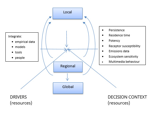
Figure 1 - Text Equivalent
Figure 1 shows the factors that play a role in the decision of whether local exposure modelling is insufficient and if regional- and global-scale exposure modelling is warranted. The elements that go into the decision and that must be available and that require integration are:
- Empirical data
- Models
- Tools
- People
The elements of the chemical and emission scenario(s) that need to be considered when making the decision are its:
- Persistence
- Residence time
- Potency
- Receptor susceptibility
- Emissions data
- Ecosystem sensitivity
- Multimedia behaviour
In addition, the figure highlights the decision context and the availability of resources as factors to consider when deciding if local exposure modelling is insufficient and if regional- and global-scale exposure modelling is warranted.
The discussion then considered 3 angles to answer the question of when it is appropriate to predict environmental concentrations beyond the local scale.
1. Availability of developed science and models for the decision context
First is the availability of developed science and models to the particular situation that is to be assessed. MB models should only be applied to those chemicals within the model’s domain, although there is no consensus on how to define domain. Further work on developing an understanding of model domain is warranted. Currently, MB models are best developed and practitioners have the greatest experience with nonpolar organic compounds (such as POPs). Several models have been developed, and there is some experience with the application of MB models to ionogenic compounds such as pharmaceuticals (Armitage et al., 2013; Csiszar et al., 2011; Franco & Trapp 2010; Trapp et al., 2010). A few models have also been developed to consider parent and transformation products where a linked consideration of these related compounds is needed to give a full assessment of the parent compound (Fenner et al., 2008; Gandhi et al., 2006). Some work has been done to extend MB model applicability to UVCBs. The SC noted that ECCC has invested in the development of models and approaches for ionizable substances. The SC advised that ECCC could promote the uptake of this approach to other models (for example, the EUSES). More generally, the SC suggested that ECCC support the scientific development needed to extend MB models to other types of substances outside the current domain of applicability.
2. Choice of appropriate models and approaches for each specific case
Second, the SC discussed if and how assessors choose the appropriate models and approaches for each specific case. The SC considered the practicality, predictability, and reproducibility of the results obtained from choices made as to which model(s) to run. The SC discussed 2 approaches that could be taken. One approach, consensus modelling (Ring et al., 2019), would be to obtain a more comprehensive set of results for a chemical by running numerous models. This approach would require investing in the training of assessors on how to use each model and how to interpret the results. This approach, of running multiple models, is possible because model run time is short given the latest developments in models and information technology infrastructure. The SC indeed noted that once in place, running a model is constrained by data but not by computational ability. As such, some members of the SC believed that given the low expense of running models, several models (or at least a more complete multi-scale model) should be run in all cases, unless this obviously does not make sense (for example, the chemical is outside the domain of applicability; the chemical does not exhibit multimedia behaviour). The advantage of this approach is obtaining copious model results, which could give insights that had not heretofore been considered. The disadvantages are the amount of data required to run the model(s) and time needed to interpret the results, and that the results could be overwhelming for the assessors given the copious model results.
The other option to guide which model(s) to run is to take a “fit-for-purpose” approach in which the use of a model(s) is clearly directed by the question(s) asked. This approach would follow a “decision tree” where, following a number of key questions, specific models would be run (Figure 2). The SC devoted some time to develop the main elements of such a decision tree. Below we present some points to illustrate the concept and to provide a starting point to the GoC, rather than to represent a definite proposal.
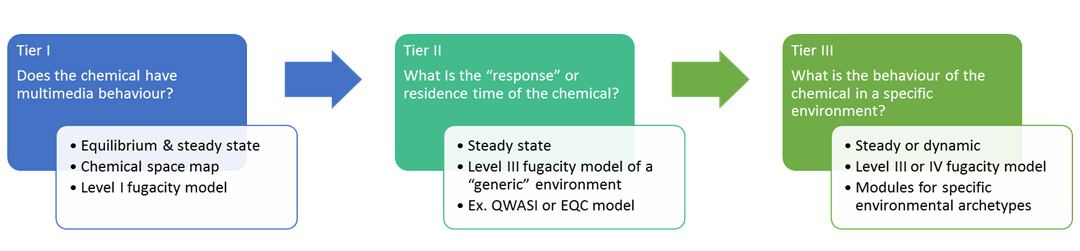
Figure 2 - Text Equivalent
Figure 2 reflects the decision tree to guide a tiered approach to using mass balance model(s) as needed. Tier I is the simplest level of consideration. Tier I is used to determine if the chemical exhibits multimedia behaviour, i.e., the chemical is found in air, water, soil. The tools for making this decision are simple equilibrium and steady-state models such as a level I fugacity model. As an alternative, a chemical space map can be used to make this decision if the chemical’s physical-chemical properties are within the map’s domain. Movement from Tier I to Tier II is warranted if the chemical exhibits multimedia behaviour. The modelling tools for use in Tier II are steady-state, non-equilibrium mass balance models such as a level III fugacity model of a "generic environment". Examples of such models are the QWASI (Quantitative Air, Water, Sediment Interaction) or EQC Model (EQuilibrium Criterion) models. Finally, movement from Tier II to Tier III is warranted if the chemical exhibits a long response or residence time in the Tier II model(s). Tier III involves the most complex model(s) that could assume either steady-state or dynamic (time dependent) conditions such as a level III or IV fugacity model. Unlike the Tier II model, the Tier III model might consider a specific environmental archetype(s) to provide a more realistic rather than generic assessment of environmental behaviour, as occurs with Tiers I and II.
Movement from Tier I to Tier II is warranted if the chemical exhibits multimedia behaviour. Movement from Tier II to Tier III is warranted if the chemical exhibits a long response or residence time.
Abbreviations: EQC, EQuilibrium Criterion; QWASI, quantitative air, water, sediment interaction.
The first tier (Tier I) is to determine if a chemical has multimedia behaviour that merits the use of a multimedia rather than single-medium model. The starting point is a chemical’s physical–chemical properties. Here, a chemical space analysis can guide decisions, noting that the chemical space needs to be extended to include the physical–chemical properties of a wider variety of chemicals such as ionogenic species and should consider methods to include UVCBs. For example, Figure 3 presents a “chemical space” diagram by plotting KAW (partition coefficient between air and water) versus KOW (partition coefficient between octanol and water) or Kd (soil–water partition coefficient). Inherent to the success of this first step is the availability of reliable physical–chemical property data.
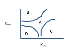
Figure 3 - Text Equivalent
Figure 3 shows a highly simplified, illustrative chemical space diagram to assess at Tier I whether a chemical will exhibit multimedia behaviour. In this case, the chemical space is defined by KAW (partition coefficient between air and water) versus KOW (partition coefficient between octanol and water). Chemicals with intermediate Kow and intermediate KAW (indicated by "A" at the centre of the chemical space map) are most likely to experience multimedia behaviour after emission and thus merit consideration using Tier II tools. Chemicals with high KAW and low KOW ("B" in the upper left corner) are expected to be found in air where atmospheric fate is important. Chemicals with high Kow and low KAW ("C" in the lower right corner) are likely to be found in "condensed" media such as soil, sediment and vegetation. Consideration using Tier II tools is recommended because of the long response time (i.e., persistence) in the environment. Finally, chemicals with low KOW and low KAW ("D" in the lower left corner) are expected to be found in water where aquatic fate is important.
Abbreviations: KAW, partition coefficient between air and water; KOW, partition coefficient between octanol and water.
Chemicals in Zone A are likely to exhibit multimedia behaviour whereas chemicals in Zone B are most likely to be found in air where atmospheric fate is important. Chemicals in Zone D are likely to be found in water where aquatic fate is important. Chemicals in Zone C are likely to be found in “condensed” media such as soil, sediment and vegetation. Here, use of a multimedia model should be considered to estimate chemical fate and distribution from point of emission to accumulation in condensed media. The SC discussed the simple Quantitative Air Water Sediment Interaction (QWASI) model developed by Mackay and colleagues (Mackay & Diamond, 1989; Mackay et al., 2014). The EQuilibrium Criterion (EQC) model, also developed by Mackay and colleagues, could also be used where the model considers chemical partitioning and fate in a “unit world” multimedia environment (Hughes et al., 2012; Mackay et al., 1996a; Mackay et al., 1996b).
For the next tier, Tier II, information should be sought on chemical response time. The response time, or “residence time,” gives information on the time to recovery (reduction in environmental concentrations) if emissions ceased. For Tier II, the mode of entry is important and could govern which compartment is of concern due to chemical accumulation and a long response time. Regional or global modelling is indicated if the response time is long (that is, the chemical is persistent). Also, if the residence time is long, then the hazard assessment needs to consider chronic effects. If the residence time is low enough, then there is no need to move to the next tier unless the chemical transforms to persistent and/or toxic by-products. Information on response time can be obtained from the models mentioned above, which are all steady-state models (no change with time). Despite the models assuming a steady state, information on chemical response or residence time can be obtained without increasing the complexity inherent in an unsteady-state or dynamic model.
Tier III involves more case-specific considerations. This is discussed at great length under Charge Question 2. For example, Tier III models could consider sensitive ecosystems, and regional and global considerations, including considerations of vulnerable populations, sensitive species, biodiversity, or endangered species. In terms of the overall workload, this should be a smaller group of chemicals because of the heavy data requirements and need for modelling expertise. For this tier, specific data that are needed include:
- site(s)-specific information about the physical environment, such as rain rate, length of vegetation growing season, snowfall, and air flow
- information about the food web
- distance from emission source to specific environment under consideration (for example, the Arctic)
Obtaining site-specific data with which to parameterize the model could be difficult. In the context of risk assessments that would lead to formal regulatory decision-making, data requirements and assumptions made are more critical and require a more in-depth analysis and justification than when used for prioritization.
The tiered/decision-tree approach, as described here, illustrates that many tools and approaches are available and can be organized in a systematic way.
3. Drivers for predicting environmental concentrations beyond local scale
The third aspect to the Charge Question is that model selection be guided by the decision context and the availability of suitable data. For prioritization, running several models in a batch approach would be feasible and useful in terms of prioritizing chemicals that might occur in the far field (see below for the tie-in with monitoring work). Exposure modelling can be particularly helpful in prioritizing industrial chemicals where specific use is often only known partially and where the hazard properties are often not fully characterized because of a lack of information. In this batch approach, generic assumptions can be made, and the margin of tolerable error is higher. Using exposure to prioritize further work where there is lack of data speaks well to the risk-based approach, which is one of the pillars of the CMP. Here, as in other instances, the consideration of exposure and hazard needs to be done in tandem. Alternatively, the assessment could be conducted in the context of regulatory decision-making where the model(s) are intended to provide greater insight into a chemical’s environmental behaviour, facilitate the interpretation of monitoring data, and allow assessors to investigate various scenarios.
Charge Question 2: How can the GoC better integrate chemical fate at relevant spatial and temporal scales to reduce key uncertainties in predicted environmental concentrations for both prioritization and risk assessment activities?
Under Charge Question 1, the SC discussed either using a battery of models or taking a tiered approach with the use of a sequential set of models, depending on the context under consideration. For Charge Question 2, the SC discussed, but did not decide upon, the strategy of taking a tiered approach versus running a battery of models as a first step. The SC then deliberated on the model(s) that would be used under either scenario and how the GoC could acquire the models and expertise needed to run them.
If a tiered approach is taken, then the approaches and models that could be used are shown in Figure 2. These steps follow those proposed by Don Mackay in his suite of fugacity models that progress from a simple Level I that illustrates the partitioning behaviour of a chemical in a defined “unit” world, to a Level III model that considers chemical behaviour assuming a steady state (for example, QWASI or EQC), to a more detailed, “site-specific” treatment of the environment at the third tier (for example, specifically parameterized QWASI, EQC, ChemCAN models). Taking this approach would require the GoC to maintain these models, which could either be independent or part of a progression of models sharing similar, fundamental calculations and parameterizations.
If a single, initial run is used, then either a battery of models or modules within a single model structure could be used, or a nested model could be used where the model incorporates different environments. An example of a model with nested architecture is SimpleBox (a multimedia environmental fate model). However, the SC commented on the challenges of maintaining a single, large model.
Regardless of whether a nested model or series of models are used, the following points were raised to enable the GoC to move towards improving their incorporation of MB modelling into its risk assessment “tool box.”
1. Develop and support a series of MB models taken from existing and emerging exposure science
The SC noted that many models are available. Thus, MB models used now by the GoC requires maintaining existing models and considering drawing new knowledge and modelling concepts from emerging exposure science.
As discussed under Charge Question 1, either a battery of models or a single, more complex model could be run, or the assessor could take a tiered approach. Both approaches require that the GoC could support a series of models. As noted above, it may be disadvantageous to support a single (and likely complex) model that would require significant effort to maintain. Alternatively, the SC considered it desirable to support a series of models that could be used as needed or to support a model consisting of modules that can be independently updated, refined, and kept current.
The SC also discussed the GoC developing and maintaining a “CMP model.” The RAIDAR (Risk Assessment IDentification And Ranking) system of models developed by Arnot and colleagues would be a candidate for adoption, given the ability of RAIDAR to estimate far- and near-field exposures to ecosystem and human receptors (Arnot & Mackay, 2008; Li et al., 2018).
Either way, the model(s) require some maintenance. As the science evolves, so too should the algorithms in the models. As knowledge of environmental systems and conditions increases, libraries of systems can be developed to parameterize the models for case-specific conditions. Computer coding formats also change over time and require ongoing efforts to maintain compatibility and accessibility. The SC noted that all these enhancements require resources.
2. Develop datasets to support the use of models
The SC emphasized that model output rests on sound model inputs. As such, datasets of inputs must be advanced and maintained. The main datasets that must be developed and maintained are the following:
- Physical–chemical properties [that is, solubility, pKa, partition coefficients, distribution ratios]. Assessors already avail themselves of QSARs to obtain estimates of physical–chemical properties, noting constraints given by domains of applicability. Examples of programs that have (and could be) used are Estimation Program Interface (EPI) Suite, United States (U.S.) Environmental Protection Agency (EPA) Chemistry Dashboard, SPARC Performs Automated Reasoning in Chemistry (SPARC), and Absolv.
- Degradation half-life data. Except for Level I models, degradation half-life data are required for model simulations, yet there are no QSARs or tools available for predicting half-lives in water, soil, and sediment for a range of chemistries. The most accessed tool for degradation half-life data is EPI Suite; however, it does not explicitly predict environmental half-lives. The CATALOGIC model is also available for estimates of soil biodegradation half-lives; however, it is proprietary. The BioWin module in EPI Suite predicts information on chemical biodegradability, but aerobic biodegradation half-lives in water are extrapolated and not directly predicted by the QSARs. Furthermore, rules of thumb are then required for extrapolating the extrapolated half-lives in water to half-lives in soil and sediment (for example, options such as 1:1:4 or 1:2:9 ratios can be applied, but with very limited scientific justification). The EPI Suite sub-model BioHCWin is the only QSAR in EPI Suite that explicitly predicts aerobic half-lives in water, but the applicability domain of this QSAR is for hydrocarbons only.
The most commonly available biodegradation studies are for ready biodegradability, and this test likely underestimates degradation (it over-estimates half-life). Higher-tier tests have been performed for fewer chemicals, and accessing those studies is more challenging when attempting to model many chemicals. Even fewer test results are available to attempt to directly address soil/sediment half-lives with experimental data or to determine what/whether degradants should be modelled. Finding degradation data for atmospheric half-lives can also be challenging. - Emissions (discussed below).
- System attributes (discussed below).
3. Integrate, in an iterative fashion, the use of models and monitoring data to support each other
The SC considered this an important point that has not necessarily been stated by other bodies that have discussed the use of models in a regulatory environment. The GoC supports several environmental monitoring efforts by ECCC and others. Monitoring data have and continue to provide an “early warning” sign of chemical movement beyond what was expected. A prime example is of the monitoring efforts conducted by the GoC in the Arctic; for example, under the Northern Contaminants Program (Government of Canada, 2018). Alternatively, screening-level models can suggest candidate chemicals that could have, for example, long-range transport (for example, Wania, 2003).
The SC commented that it is important to continue this productive interplay between the use of models and monitoring data to identify chemicals likely to have or that have been found to exhibit multimedia behaviour and/or long-range transport potential.
Other jurisdictions have developed user-friendly online databases [for example, the Information Platform for Chemical Monitoring (IPCHEM)];) to fill knowledge gaps on chemical exposure and its burden on health and the environment. The GoC and provinces spend considerable resources obtaining chemical measurements in environmental media. These data are extremely valuable for addressing data gaps on chemical exposure and for fate and transport model evaluations. Initial efforts to organize this information obtained by the GoC could evolve to produce an evergreen and publicly accessible monitoring database for Canada.
4. Develop and maintain in-house expertise with model development and maintenance. Develop strategic partnerships to promote model development and adoption
Achieving the advances outlined in the above point 1 relies on curating and maintaining models chosen for support by the GoC. The GoC also needs to keep abreast of new developments in fate and exposure modelling and assess their possible adoption into programs such as the CMP. For this approach to succeed, the SC discussed maintaining a steering committee with oversight of the GoC’s modelling needs and available models, and keeping abreast of new developments.
The SC then discussed the options of relying on “in-house” versus external expertise in model development and maintenance. These 2 options are not necessarily mutually exclusive. The GoC could provide ongoing support and open lines of communication with independent model developers in the research and consulting community and other (international) regulatory authorities. The advantage here is that the work is ongoing, and innovations can take place because model development is not necessarily constrained by “fit-for-purpose” use. The potential disadvantages are the lack of control, potential loss of continuity, and the inability for the GoC risk assessors to have immediate access to modelling expertise.
Thus, to add to the existing reliance on external expertise, the SC considered that the GoC develop “in-house” expertise in model development and maintenance. Having some in-house expertise would be necessary if the GoC is to maintain a suite of models. The in-house expert(s) would ensure that the model(s) are kept up to date and would serve as a resource to chemical assessors. The latter point bears some explanation. If indeed the GoC adopts the greater use of models to assess far-field exposure, then the risk assessors would require training and “back up” to ensure that model use is consistent with the assumptions, domain of applicability, and so forth, and that the results are appropriately interpreted. Thus, model adoption will require not only GoC efforts to support the models but also appropriate usage assurance.
5. Use case studies to guide model development and implementation
The recommendation of using case studies is an ongoing theme with questions tackled by the SC (for example, see Public Health report). Here, the use of case studies is intended to test and to gain experience with the use of MB models for assessment purposes. The SC did not go into detail regarding the types of case studies that should be conducted, but did note that the case studies need to consider the wide range of physical–chemical properties encountered, consider a generic versus specific archetype to typify model environments, and take into account the wide range of emission scenarios. Case studies should include data-rich chemicals, such as pesticides. Focusing a case study on a legacy chemical can also provide insights, including a degree of model evaluation. Generally, problem-driven development and evaluation of models and modelling approaches will ensure that resources are focused on the greatest assessment needs of the GoC.
Further Considerations
The SC went into further detail on the “how-to” of model development and application.
Emissions
A key requirement—and also a major uncertainty—in fate and exposure model predictions for concentrations in the environment is emission rate and location information. A multitude of emissions information (notably the medium to which emission occur, geographic locations, magnitude of the type(s) of emissions, and temporal emission trends) is critical for running and correctly interpreting model results beyond the simple models used to determine partitioning and whether a chemical has multimedia behaviour (for example, a Level I model). Despite the need for emission data, these are often the least well known of all model inputs. Thus, the SC was clear on the need to improve the estimates of emissions which underpin model results.
One way to avoid uncertainty in emissions information is to avoid using emissions rates and rather to run a model with a unit emission to a given medium or media. Here, a unit emission refers to a hypothetical emission such as 1 mol/h into a region. Running a model in this way could assist with prioritization. Beyond prioritization, models can be run in reverse (inverse modelling) to obtain aggregate emission estimates based on measured concentrations (for example, Diamond et al., 2010). This presents another case where monitoring and modelling require integration. The advantage of inverse modelling is obtaining “order-of-magnitude” estimates of emissions that are case specific. The disadvantage comes in not knowing necessarily the medium to which a chemical is emitted and attributing sources to those emissions. The capacity to operationalize inverse modelling and reduce uncertainty in fate model calculations is predicated by suitable and reliable monitoring data (see previous point).
The SC recommended that the collection of emissions data be prioritized. Those emission data are needed across the chemical’s life cycle, including end-of-life (not including landfills). The SC also suggested developing emission scenario data for data-rich and data-poor substances. Models that can predict chemical emission rates [for example, CiP-CAFE (Li, Arnot, & Wania, 2018a, 2018b; Li et al., 2017; Li & Wania, 2016)] should be evaluated and refined as necessary.
System attributes
Beyond the simple models needed for Tier I or II, the SC discussed the attributes or properties needed for a Tier III model(s). The following suggestions were made that would provide for system attributes tailored to the Canadian environment.
- A series of “functional” systems. Here, a “functional” system is an environment or a system that provides a common function. A non-exhaustive series of examples include:
- urban areas that provide the function of human settlement and activities
- an agricultural ecosystem, where a prairie system could include a slough that supports wildlife
- an arctic ecosystem, because of its unique sensitivity as an ecosystem and as an indicator of long-range transport (the SC discussed that there may be other functional ecosystems that are of importance such as a prairie slough, which is also a sensitive ecosystem indicative of agricultural activities)
- Geographically specific ecozones. These are represented in ChemCAN (Webster et al., 2004; Woodfine et al., 2002). This type of model could be updated by linking with geographic information system information. The SC recognized that updating the ecozones, including the general parameterization and also that of ecozone-specific food webs, requires research and development
- Parameterization within the functional systems and/or ecozone that includes extreme events and conditions (for example, droughts and floods). Here, the SC noted that model parameterizations need to keep abreast of environmental change, where exposures occurring during extreme events should be considered in addition to “average” environmental conditions. Extreme conditions should be important to consider with “high-consequence” emissions
- Differing geographic scales from local, to regional/watershed, to global
Expressing uncertainty
The SC discussed the importance of capturing and expressing the uncertainty in model estimates. The discussion did not go into detail about how best to capture uncertainty other than to note that it is now common to run models that include the probability distributions of various parameters in order to generate probability distributions of output data.
Another aspect of uncertainty in modelling is the need to judge the quality of input data. The SC raised the idea of developing guidance on evaluating data quality.
Model evaluation
Model evaluation remains an important aspect of model development and use. The SC discussed various aspects of model evaluation, including the correct terms that should be used (see Oreskes et al., 1994). Although MB models are based on fundamental physical processes, there remains considerable uncertainty in correctly capturing environmental processes and parameterization.
Model evaluation could be part of the activities undertaken to maintain models used by the GoC. Here, monitoring data can enable model evaluation; thus, again it points to the need to integrate chemical monitoring and modelling activities.
Charge Question 3: What are the primary advantages/disadvantages and key uncertainties the GoC might expect from implementing dynamic and more spatially resolved exposure assessment approaches for CMP chemical evaluation? Describe ways to overcome these disadvantages.
The SC discussed many advantages and disadvantages of integrating exposure modelling into ecosystem risk and far-field human health assessments. The discussion also included major uncertainties.
Advantages
- Can address the extensive exposure data gaps that result in uncertainty in basic knowledge of chemicals in the environment and the capacity to conduct chemical risk assessments
- Can extend the analysis of exposure beyond the persistent and bioaccumulative approach to give additional lines of evidence, leading to an increased of level of protection for the environment and human health
- Can lead to more transparent analysis and ability to communicate results to the public and stakeholders
- Can assist not only with exposure-based prioritization of substances with CMP and exposure-based prioritization of data needs, but also supports risk-based decision making
- Can assist with global efforts towards chemical management through, for example, the United Nations Environment Programme or the Stockholm Convention on Persistent Organic Pollutants
- Can provide the capacity for integration of scientific knowledge from multiple disciplines along with the assembly of data from multiple sources where the integration itself can provide new insights beyond that obtained from individual disciplines
- An initiative to further advance the incorporation of modelling into exposure assessment could provide opportunities for global leadership in this area, as Canada has been a leader in exposure modelling in the past
- In terms of the insights gained, exposure modelling can improve the knowledge of:
- greater realism in exposure estimates and scenarios than is currently the case, and hence, improved confidence of estimates used in risk assessments
- main processes and mechanisms responsible for fate
- future forecasts, given changes in emissions, environmental conditions, and so forth
- estimates of system recovery times
Last, the SC commented that many models are currently available to expedite their use in exposure modelling. A strategy for their use is required, which could build from experience (both in-house and with collaborators).
Disadvantages
- May increase data needs (including, in some cases, data on emissions)
- May questionably lead to an increase in false positives and/or false negatives
- Can lead to probabilistic model results that are difficult to interpret and communicate to the public and stakeholders (although issues of dealing with uncertainty pertain to both exposure and hazard assessments)
- Require additional and on-going expertise, and thus additional resources (models should be kept updated and curated)
Key uncertainties
Although there are many uncertainties associated with modelling and model input data, the SC recognized that modelling also enables the prioritization of those uncertainties by conducting a sensitivity analysis. Indeed, in the absence of a model, the relative importance of narrowing specific uncertainties cannot be judged.
The greatest uncertainty facing model application lies in emissions, which are difficult to quantify, and thus, rarely well characterized. This uncertainty was discussed under Charge Question 2 and is mentioned below as an area requiring research and development. The SC discussed strategies for obtaining data from businesses, while noting that complex supply chains and proprietary formulation data can make it difficult to obtain reliable and accurate data.
Solutions for overcoming challenges
The following were offered as strategies for overcoming the disadvantages associated with incorporating models into exposure assessment:
- Develop models and gather data according to defined problems (fit-for-purpose)
- Offset to some extent the monetary investment of incorporating exposure models by developing strategic partnerships to share the financial responsibilities
- Demonstrate the strength and advantages of incorporating exposure modelling by using case studies that illustrate the “value added”
- Better integrate sectoral collaboration among the GoC, provincial counterparts, academia, and consulting (this collaboration holds for sharing modelling expertise as well as integrating modelling and monitoring/measurement data)
- Invest in “in-house” modelling expertise and/or training and for integrating the considerable data gathered by the GoC into a curated, centralized database
- Incentivize for businesses the case for estimating emissions information, which will allow the GoC to move to more realistic scenarios rather than “worst-case” scenarios that are often currently run out of necessity
The SC recognized that Canada plays a leading role as a regulatory authority in the development of environmental exposure models and could further support the development and evolution of such. Strategic partnerships with academia and other authorities could strengthen this leading role. In this context, the possible alliance between ECCC and the European Union/Organisation for Economic Co-operation and Development (EU/OECD) (specifically in the context of EUSES/Chesar software developments) could lead to a robust implementation of the science developed under the leadership of Canada in the integrated tools that EU/OECD develops models and promotes their free use.
The SC also discussed specific areas that would benefit from research and development, some of which were mentioned in previous sections of this report:
- Expand the domain of chemicals for which the models are applicable to include, for example, ionogenic compounds, UVCBs, linked parent and transformation products
- Develop data infrastructure and methods for estimating emissions. The SC wanted to emphasize that the lack of emissions data is the weakest link in the entire modelling enterprise
- The SC suggested that new approaches such as “CiP-CAFE” (Chemicals in Products–Comprehensive Anthropospheric Fate Estimation, a dynamic substance flow model) could be pursued
Finally, the SC organized activities of an implementation strategy into short-, medium-, and long-term efforts needed to implement the improved use of exposure models under CMP:
- Short-term:
- system development
- data organization and integration
- identify data and approaches for integration
- invest in resources to operationalize modelling effort, including developing basic in-house expertise and training
- integrate measurement (monitoring) and modelling efforts
- Medium-term
- data support (for example, development of data infrastructure as discussed above)
- expand the domain of substance applicability
- refining of conceptualization and parameterization of functional systems (for example, urban, agricultural) and ecozones for use in higher-tiered model(s)
- Long-term
- develop new models and/or enhancements for existing models (for example, linking parent and transformation products)
- continue to expand the system to consider, for example, UVCBs, other functional systems, and more complete emissions scenarios
- build confidence with model expertise and applications
Conclusions
The SC appraised the strengths, weaknesses, and approaches for integrating fate and exposure models to compliment or enhance current efforts for ecosystem risk assessment and for assessing far-field human exposures. The SC expressed a consensus view that increasing incorporation of MB modelsinto current assessment would be of benefit for numerous reasons. The SC did not arrive at a clear path for implementation, but rather suggested options for implementing the expanded use of exposure models. Below we summarize the main points from the 2 day discussion on exposure modelling.
- The SC derived a list of characteristics of substances that can act as a guideline for determining when a multimedia exposure modelling approach is warranted.
- After determining that a multimedia approach is warranted, the SC provided 2 options for guiding which model or models could be used: (1) taking a tiered approach to determine which level of complexity is needed for the situation (fit-for-purpose), or (2) run a battery of models or a single, nested model to provide comprehensive information on chemical fate. Both options have their advantages and disadvantages.
- The following needs were identified for bringing exposure modelling into the current risk assessment approach:
- Develop and support a series of MB models taken from existing and emerging exposure science
- Support efforts to collate existing data to support the use of models and integrate monitoring (data gathering) and modelling efforts
- Support efforts to collect priority data required as model inputs and parameters (for example, collect data to improve emissions estimates, which are the most significant data gaps constraining model application; create databases and QSARs for degradation half-lives)
- Support work on extending the domain of MB models from “classical” nonpolar organic compounds to include, for example, ionogenic, UVCBs, dyes and pigments, organic salts and organometallics, and some polymers
- Consider supporting in-house modelling expertise as well as fostering collaborations and strategic partnerships among sectors within and beyond Canada to support model development and application
- Consider strategic partnerships with academia and other authorities. For example, a possible alliance between ECCC and the EU/OECD (specifically in the context of the EUSES/Chesar software developments) could lead to a robust implementation of the science developed under the leadership of Canada
- Consider supporting development of a higher-tiered model(s) with modules tailored to the diversity of Canadian environments in terms of functions (for example, urban, agriculture), ecozones, temporal variations in emissions, and changes (including the consideration of extreme events)
- Develop experience with expressing uncertainty from model estimates and model evaluation
- Use case studies to guide model development and implementation
- Integrate model development and chemical monitoring/surveillance to optimize the value of each
- The SC listed numerous advantages to increasing incorporation of MB modelsinto current assessment as well as disadvantages, some key uncertainties, and solutions for overcoming the challenges associated with using exposure models. The SC also commented on activities that could be taken in the short-, medium-, and long-term as part of an implementation strategy.
Glossary
- ChemCAN
- a Level III chemical fate model of 24 regions of Canada
- CiP-CAFE
- Chemicals in Products–Comprehensive Anthropospheric Fate Estimation
- CMP
- Chemicals Management Plan
- ECCC
- Environment and Climate Change Canada
- EQC
- EQuilibrium Criterion
- EU
- European Union
- EUSES
- European Union System for the Evaluation of Substances
- GoC
- Government of Canada
- MB
- mass balance, in the context of the type of model discussed
- OECD
- Organisation for Economic Co-operation and Development
- PBT
- persistent, bioaccumulative, and toxic, in the context of criteria for categorizing chemical toxicity
- POP
- persistent organic pollutant, as defined by the Stockholm Convention
- QWASI
- quantitative air, water, sediment interaction
- SC
- Science Committee
- UVCB
- unknown or variable composition, complex reaction products, and biological material
- vPvB
- very persistent and very bioaccumulative
References
Armitage, J. M., Arnot, J. A., Wania, F., Mackay, D. 2013. Development and evaluation of a mechanistic bioconcentration model for ionogenic organic chemicals in fish. Environ Toxicol Chem, 32:(1), 115–128.
Arnot, J. A., Mackay, D. 2008. Policies for chemical hazard and risk priority setting: can persistence, bioaccumulation, toxicity and quantity information be combined? Environ Sci Technol, 42(13): 4648-4654.
Arnot, J. A., Mackay, D., Sutcliffe, R., Lo, B. 2010. Estimating farfield organic chemical exposures, intake rates and intake fractions to human age classes. Environ Model Software, (25): 1166-1175.
Bonnell, M. A., Zidek, A., Griffiths, A., Gutzman, D. 2018. Fate and exposure modeling in regulatory chemical evaluation: new directions from retrospection. Environmental Science: Processes & Impacts, 20(1): 20-31.
Csiszar, S. A., Gandhi, N., Alexy, R., et al. 2011. Aquivalence revisited—New model formulation and application to assess environmental fate of ionic pharmaceuticals in Hamilton Harbour, Lake Ontario. Environ Int, 37(5): 821-828.
Diamond M. L., Melymuk L., Csiszar S. A., Robson M. 2010. Estimation of PCB stocks, emissions, and urban fate: will our policies reduce concentrations and exposure? Environ Sci Technol, (44): 2777-2783.
European Chemicals Agency [ECHA]. 2018. Workshop on EUSES update needs.
Fenner, K., Schenker U., Scheringer M. 2008. Modelling environmental exposure to transformation products of organic chemicals. In A. B. A. Boxall (Ed.), The Handbook of Environmental Chemistry: Vol. 2. Transformation products of synthetic chemicals in the environment (pp. 121-149)..
Franco, A., Trapp, S. 2010. Multimedia activity model for ionizable compounds—Validation study with 2,4-D, aniline and trimethoprim. Environ Toxicol Chem, 29(4): 789-799.
Government of Canada. 2018. Northern Contaminants Program—Background.
Hughes, L., Mackay, D., Powell, D. E., Kim, J. 2012. An updated state of the science EQC model for evaluating chemical fate in the environment: Application to D5 (decamethylcyclopentasiloxane). Chemosphere, 87(2): 118-124.
Isaacs, K. K., Glen, W. G., Egeghy, P., et al. 2014. SHEDS-HT: An integrated probabilistic exposure model for prioritizing exposures to chemicals with near-field and dietary sources. Environ Sci Technol, 48(21): 12750-12759.
Li, L., Arnot, J. A., Wania, F. 2018a. Revisiting the contributions of far- and near-field routes to aggregate human exposure to polychlorinated biphenyls (PCBs). Environ Sci Technol, 52(12): 6974-6984.
Li, L., Arnot, J. A., Wania, F. 2018b. Towards a systematic understanding of the dynamic fate of polychlorinated biphenyls in indoor, urban and rural environments. Environ Int, (117): 57-68.
Li, L., Liu, J. G., Hu, J. X., Wania, F. 2017. Degradation of fluorotelomer-based polymers contributes to the global occurrence of fluorotelomer alcohol and perfluoroalkyl carboxylates: A combined dynamic substance flow and environmental fate modeling analysis. Environ Sci Technol, 51(8): 4461-4470.
Li, L., Wania, F. 2016. Tracking chemicals in products around the world: Introduction of a dynamic substance flow analysis model and application to PCBs. Environ Int, (94): 674-686.
Li, L., Westgate, J. N., Hughes, L. 2018. A model for risk-based screening and prioritization of human exposure to chemicals from near-field sources. Environ Sci Technol, 52(24): 14235-14244.
Mackay, D., Di Guardo, A., Paterson, S., Cowan, C. E. 1996a. Evaluating the environmental fate of a variety of types of chemicals using the EQC model. Environ Toxicol Chem, 15(9): 1627-1637.
Mackay, D., Di Guardo, A., Paterson, S., Kicsi, G., Cowan, C.E., Kane, D. M. 1996b. Assessment of chemical fate in the environment using evaluative, regional and local-scale models: Illustrative application to chlorobenzene and linear alkylbenzene sulfonates. Environ Toxicol Chem, 15(9): 1638-1648.
Mackay, D., Diamond, M. 1989. Application of the Qwasi (quantitative water air sediment interaction) fugacity model to the dynamics of organic and inorganic chemicals in lakes. Chemosphere, 18(7-8): 1343-1365.
Mackay, D., Hughes, L., Powell, D. E., Kim, J. 2014. An updated Quantitative Water Air Sediment Interaction (QWASI) model for evaluating chemical fate and input parameter sensitivities in aquatic systems: Application to D5 (decamethylcyclopentasiloxane) and PCB-180 in two lakes. Chemosphere, (111): 359-365.
National Academies of Sciences. 2017. Using 21st Century Science to Improve Risk-Related Evaluations. The National Academies Press: Washington, DC; p. 260.
Oreskes N., Shrader-Frechette K., Belitz K. 1994. Verification, validation, and confirmation of numerical models in the earth sciences. Science, 263(5147): 641-646.
Ring C. L., Arnot J. A., Bennett D. H., et al. 2019. Consensus modeling of median chemical intake for the U.S. population based on predictions of exposure pathways. Environ Sci Technol, 53(2):719-732. doi: 10.1021/acs.est.8b04056. Epub 2018 Dec. 24.
Trapp, S., Franco, A., Mackay, D. 2010. Activity-based concept for transport and partitioning of ionizing organics. Environ Sci Technol, (44): 6123-6129.
Vermeire, T. G., Jager, D. T., Bussian, B., et al. 1997. European Union system for the evaluation of substances (EUSES). Principles and structure. Chemosphere, 34(8): 1823-1836.
Vermeire, T. G., Rikken, M., Attias, L., et al. 2005. European Union system for the evaluation of substances (EUSES): The second version. Chemosphere, (59): 473-485.
Wania, F. 2003. Assessing the potential of persistent organic chemicals for long-range transport and accumulation in polar regions. Environ Sci Technol, (37): 1344-1351.
Webster, E., Mackay, D., Di Guardo, A., Kane, D., Woodfine, D. 2004. Regional differences in chemical fate model outcome. Chemosphere, (55): 1361-1376.
Woodfine, D., MacLeod, M., Mackay, D. 2002. A regionally segmented national scale multimedia contaminant fate model for Canada with GIS data input and display. Environmental Pollution, (119): 341-355.