
Technical Guidance for Assessing Cumulative Environmental Effects under the Canadian Environmental Assessment Act, 2012
This document provides guidance on federal environmental assessments commenced under the former Canadian Environmental Assessment Act, 2012. It is retained for the completion of transitional environmental assessments commenced prior to the Impact Assessment Act. For more information on transitional environmental assessments, please consult the Legislation and Regulations page.
Interim Technical Guidance
March 2018
Version 2
Acknowledgements
The Agency would like to acknowledge the many valued contributions from experts and environmental assessment (EA) practitioners that have informed the content of this document.
These include the authors of the 1999 Cumulative Effects Assessment Practitioners’ Guide; the Cumulative Effects Assessment Working Group (G. Hegmann, C. Cocklin, R. Creasey, S. Dupuis, A. Kennedy, L. Kingsley, W. Ross, H. Spaling and D. Stalker) and AXYS Environmental Consulting Ltd. In addition, Gartner Lee Ltd., Golder Associates Ltd. and Stantec Consulting Ltd. made significant contributions to this document.
The Agency is particularly grateful to J. Barnes (Stantec Consulting Ltd.), P. Duinker (Dalhousie University), L. Hardwick (Stantec Consulting Ltd.), G. Hegmann (Stantec Consulting Ltd.), L. Greig (ESSA Technologies Ltd.), B. Noble (University of Saskatchewan & Aura Environmental Research and Consulting Ltd.), T. Skillen (Golder Associates Ltd.), J. Rice (Department of Fisheries and Oceans), B. Torrie (Canadian Nuclear Safety Commission), and M. Eyre (National Energy Board) for their contributions.
The Agency would also like to thank all those who submitted comments during the public comment period on the draft version of this document.
Document Information
Disclaimer
Please be advised that this draft guidance piece is an interim document. The Agency is currently reviewing the Environmental Assessment process and as a result of the review, EA practice, policies and procedures may change. This draft guidance document reflects current practice under the Canadian Environmental Assessment Act, 2012 (CEAA 2012). This Technical Guidance is for information purposes only. It is not a substitute for the Canadian Environmental Assessment Act, 2012 (CEAA 2012) or its regulations. In the event of an inconsistency between this document and CEAA 2012 or its regulations, CEAA 2012 or its regulations would prevail.
For the most up-to-date versions of CEAA 2012 and regulations, please consult the Department of Justice website.
Agency staff can use this document or portions of it in correspondence and share this document with external partners on an as needed basis by email, using the standard email text provided by Operational Support Directorate. For questions or further information please contact Guidance / Orientation [CEAA/ACEE] CEAA.guidance-orientation.ACEE@ceaa-acee.gc.ca
Updates
This document may be reviewed and updated periodically. To ensure that you have the most up-to-date version, please consult the Policy and Guidance page of the Canadian Environmental Assessment Agency's website.
Copyright
© Her Majesty the Queen in Right of Canada, as represented by the Minister of Environment and Climate Change, 2018.
This publication may be reproduced for personal or internal use without permission, provided the source is fully acknowledged. However, multiple copy reproduction of this publication in whole or in part for purposes of redistribution requires the prior written permission from the Canadian Environmental Assessment Agency, Ottawa, Ontario K1A 0H3, or info@ceaa-acee.gc.ca
Catalogue Number: En106-204/2018E-PDF
ISBN: 978-0-660-24634-5
Ce document a été publié en français sous le titre: Évaluation des effets environnementaux cumulatifs en vertu de la Loi canadienne sur l’évaluation environnementale (2012) – Orientations techniques intérim
Alternative formats may be requested by contacting: info@ceaa-acee.gc.ca.
This document is also available in Adobe's Portable Document Format (1.9 MB).
Table of Contents
- List of Abbreviations and Acronyms
- Introduction
- 1.0 Overview and Outcomes of Scoping
- 1.1 Identifying Valued Components
- 1.2 Determining Spatial Boundaries
- 1.3 Determining Temporal Boundaries
- 1.4 Examining Physical Activities that have been and will be carried out
- 2.0 Overview and Outcomes of the Analysis
- 2.1 Analyzing Various Types of Data and Information
- 2.2 Addressing Data Limitations and Uncertainty in the Analysis
- Appendix 1: Source-pathway-receptor Model
- Appendix 2: Types of Cumulative Effects
- Appendix 3: Methods for Cumulative Effects Assessment
List of Figures
- Figure 1. Environmental Assessment Framework and Cumulative Effects Assessment
- Figure 2. Generic Approach to Scoping for Cumulative Effects Assessment
- Figure 3. Future Scenario
- Figure 4. Example of a Matrix Structure for Outcome Documentation
- Figure 5. Source-Pathway-Receptor Model
- Figure 6. Additive Cumulative Effects
- Figure 7. Synergistic Cumulative Effects
- Figure 8. Compensatory Cumulative Effects
- Figure 9. Masking Cumulative Effects
- Figure 10. Network or System Diagram of Cumulative Effects
List of Abbreviations and Acronyms
- ATK
- Aboriginal Traditional Knowledge
- Agency
- The Canadian Environmental Assessment Agency
- CEAA 2012
- Canadian Environmental Assessment Act, 2012
- EA
- Environmental Assessment
- EIS
- Environmental Impact Statement
- GIS
- Geographic Information System
- OPS
- Operational Policy Statement
- Project
- A designated project under CEAA 2012 for which the Agency is the responsible authority
- Project EA
- EA of designated projects conducted under CEAA 2012 for which the Agency is the responsible authority
- TLU
- Traditional Land Use
- VC
- Valued Component
- ZOI
- Zone of Influence
Introduction
Context
The Canadian Environmental Assessment Act, 2012 (CEAA 2012) aims to protect components of the environment that are within federal legislative authority from significant adverse environmental effects caused by a project, including cumulative environmental effects.
In addition, CEAA 2012 ensures that a project is considered in a careful and precautionary manner to avoid significant adverse environmental effects, when the exercise of a power or performance of a duty or function by a federal authority under any Act of Parliament, other than CEAA 2012, is required for the project to be carried out.
CEAA 2012 requires that each environmental assessment (EA) of a project take into account any cumulative environmental effects that are likely to result from the project in combination with the environmental effects of other physical activities that have been or will be carried out.
Throughout the guidance, the term “environmental effects” refers to environmental effects as described in section 5 of CEAA 2012 (see description and examples below). In addition, the term “cumulative effects” refers to cumulative environmental effects as mentioned in paragraph 19(1)(a) of CEAA 2012.
Under CEAA 2012, the “environmental effects” to be considered are those in areas of federal jurisdiction as described in section 5, which include:
- effects on fish and fish habitat, shellfish and their habitat, crustaceans and their habitat, marine animals and their habitat, marine plants, and migratory birds;
- effects on federal lands;
- effects that cross provincial or international boundaries;
- with respect to Aboriginal peoples, effects of any changes to the environment on health and socio-economic conditions, physical and cultural heritage, the current use of lands and resources for traditional purposes, or any structure, site or thing that is of historical, archaeological, paleontological or architectural significance;
- changes to the environment that might result from federal decisions as well as any associated effects on health and socio-economic conditions, matters of historical, archaeological, paleontological or architectural interest, or other matters of physical or cultural heritage.
Examples of cumulative effects:
Fish & Fish Habitat: destruction of habitat of the same fish population from multiple physical activities.
Aquatic Species: shoreline destruction from multiple physical activities resulting in the removal of several patches of a marine plant.
Socio-Economic Conditions: environmental effects from multiple physical activities resulting in the decline of a bivalve population on which an Indigenous group depends as a source of income.
Physical and Cultural Heritage: damage caused to sites associated with the creation of legends, ceremonial functions, personal vision quests etc. as a result of multiple physical activities.
Current Use of Lands and Resources: effects on use of traditional fishing grounds owing to decreased fish population which results from multiple physical activities.
Archaeology: disturbance of an archaeologically significant site due to construction activities associated with multiple physical activities.
Please refer to Basics of Environmental Assessment and the Practitioners Glossary for Environmental Assessment of Designated Projects under the Canadian Environmental Assessment Act, 2012 for additional information on the EA process and key terms under CEAA 2012.
Purpose
The Operational Policy Statement on Assessing Cumulative Environmental Effects under CEAA 2012 (OPS) clarifies CEAA 2012 requirements related to cumulative effects and provides core guidance to ensure that these requirements are met in project EAs where the Agency is the responsible authority, and when the EA is conducted by a review panel.
This technical guidance document provides methodological options and considerations to support the implementation of CEAA 2012 and the approach outlined in the OPS in a way that achieves high quality EA.
This document informs the preparation of directives by the Agency, such as the Environmental Impact Statement (EIS) Guidelines, and supports proponents in the development of an EIS. It also provides guidance to Agency employees in their interactions with those engaged in federal EA, such as proponents, federal authorities, other jurisdictions, Indigenous groups, and the public.
Application
This technical guidance informs the assessment of cumulative effects undertaken as part of the EA of designated projects conducted under CEAA 2012 for which the Agency is the responsible authority. CEAA 2012 requires that an EA of a designated project take into consideration any cumulative environmental effects, which includes greenhouse gas (GHG) emissions associated with projects. This technical guidance does not apply to the assessment of cumulative effects of GHG emissions. Methodological approaches and considerations for cumulative effects assessment of GHG emissions continue to evolve. EA practitioners seeking direction on the cumulative effects assessment of GHGs under CEAA 2012 are encouraged to contact the nearest Agency regional office.
In this document, the term “project” refers to designated projects conducted under CEAA 2012 for which the Agency is the responsible authority, and “project EA” refers to the EA of designated projects conducted under CEAA 2012 for which the Agency is the responsible authority
For such a project EA, this technical guidance replaces the 1999 guide entitled “Cumulative Effects Assessment Practitioners Guide”. The 1999 guide will continue to apply for EAs initiated under the former Canadian Environmental Assessment Act that are still being conducted pursuant to the transitional provisions of CEAA 2012.
When the National Energy Board (NEB) is the responsible authority, direction and guidance can be found in the NEB filing manual. Applicants seeking guidance on nuclear projects should refer to the Canadian Nuclear Safety Commission’s regulatory framework.
This technical guidance should be used in conjunction with other Agency policy and guidance instruments. For an EA by a review panel, additional guidance and direction may be provided in the Terms of Reference or Joint Review Panel Agreement.
General Approach
The practice of EA calls for examining potential effects of a project on valued components (VCs). In the context of CEAA 2012, VCs are selected to enable identification or analysis of environmental effects as described in section 5 of CEAA 2012. This technical guidance therefore proposes a VC-centered approach for the assessment of cumulative effects.
The OPS outlines the five-step EA framework as it relates to cumulative effects assessment (see Figure 1). This document focusses primarily on steps 1 and 2, scoping and analysis. Practitioners should refer to the OPS for further guidance on steps 3-5 and also consult the Policy and Guidance page of the Agency's website for updated information as it is developed.
OPS Approach
All cumulative effects assessments should include the five steps described below - scoping, analysis, mitigation, significance, and follow up.
Figure 1. Environmental Assessment Framework and Cumulative Effects Assessment
Step 1: Scoping
Step 1 defines the scope of the assessment. This includes identifying VCs for which residual environmental effects are predicted, determining spatial and temporal boundaries to capture potential cumulative effects on these VCs, and examining the relationship of the residual environmental effects of the designated project with those of other physical activities. Scoping helps determine which VCs should be carried forward to Step 2 analysis.
Step 2: Analysis
Step 2 considers how the physical activities examined during Step 1 may affect the VCs identified for further analysis in Step 1. Step 2 addresses those VCs within spatial and temporal boundaries determined for the assessment of cumulative effects.
Step 3: Mitigation
Step 3 aims to identify technically and economically feasible measures that would mitigate adverse cumulative effects. Mitigation may include elimination, reduction or control or, where this is not possible, restitution measures such as replacement, restoration or compensation should be considered.
Step 4: Significance
Step 4 is concerned with determining the significance of any adverse cumulative environmental effects that are likely to result from a designated project in combination with other physical activities, taking into account the implementation of mitigation measures.
Step 5: Follow-up
Step 5 involves the development of a follow-up program that addresses both project-specific environmental effects and cumulative effects. A follow-up program verifies the accuracy of the EA and determines the effectiveness of any mitigation measures that have been implemented.
The detailed approach to the assessment of cumulative effects is established on a case-by-case basis taking into account:
- the project-specific EIS guidelines, direction provided by the Agency, or, for an EA by review panel, any additional guidance provided in the Terms of Reference or Joint Panel Agreement;
- the requirements of CEAA 2012 and core guidance set in the OPS; and
- the technical options and considerations presented in this guidance.
Timing for conducting the cumulative effects assessment
This guidance is consistent with the general practice that calls for first examining the environmental effects of the project in isolation (project-specific environmental effects) before moving to the consideration of other physical activities (for more information on other physical activities, see section 1.4 of this document). This allows practitioners to first consider mitigation measures for the project and determine if there are residual effects after these mitigation measures have been considered. Identifying such residual effects is one of the ways in which a practitioner can orient and focus the assessment of cumulative effects.
Nonetheless, practitioners may sometimes find it useful to conduct the assessment of cumulative effects at the same time as they are addressing the project-specific environmental effects. As a minimum, information and data needed for the cumulative effects assessment should be considered from the outset of the EA for planning purposes.
Scoping (Step 1) for the cumulative effects assessment can therefore be started during or after the assessment of potential project-specific environmental effects. In either case, as the EA advances and additional information is gained, it may become clearer which VCs should be carried forward to Analysis (Step 2). Scoping is therefore iterative, and adjustments can be made at different points during the EA process.
Scope and Organization
Most of the guidance in this document relates to the first two steps of the framework presented in the OPS. Section 1 covers scoping and Section 2 covers analysis. To facilitate future updates of this guide, each section is organized into stand-alone guidance sheets (e.g., guidance sheet 1.0, entitled “Overview and Outcomes of Scoping”, is the first guidance sheet dealing with Step 1).
Additional technical background is provided in appendices as follows:
- Appendix 1 provides information on the source-pathway-receptor model that can be used to identify the source of an environmental change, what the source may affect (receptor), and how the source may reach the receptor (pathway).
- Appendix 2 provides examples of types of cumulative effects to support the consideration of cumulative effects on VCs.
- Appendix 3 provides a brief introduction to some of the methods that may be used in conducting Step 1 (scoping) or Step 2 (analysis).
In this technical guidance, a methodology refers to a technical approach and related considerations for use in the conduct of an EA. In addition, a methodology generally frames the implementation of various methods. A “method” is a specific tool, technique, or procedure used as part of implementing the chosen methodology.
1.0 Overview and Outcomes of Scoping
As the first step in a cumulative effects assessment, scoping serves to orient and focus subsequent steps. Its overall outcome is a list of VCs that should be carried forward into the Step 2 analysis, as well as a rationale for VCs considered in scoping that are not carried forward. Scoping documents the scientific evidence and advice, as well as feedback from the public and Indigenous groups used to determine if further assessment of the VCs is warranted.
Methodologies
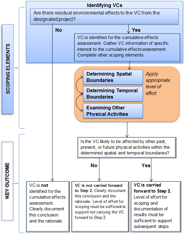
Figure 2 summarizes the recommended generic approach to scoping. The information in the following paragraphs provides an overview of the methodologies that can be used for the scoping step, starting with a description of the generic approach.
As per Figure 2, a cumulative effects assessment generally starts with addressing VCs for which residual environmental effects are predicted, after consideration of mitigation measures, regardless of whether those residual environmental effects are predicted to be significant.
For each of these VCs:
- gather information on the VC of particular relevance to the cumulative effects assessment (e.g., comments from the public, Indigenous groups, experts, government and non-governmental organizations);
- determine the spatial boundaries within which the potential for cumulative effects will be examined and, if appropriate, analyzed;
- determine the temporal boundaries within which the potential for cumulative effects will be examined and, if appropriate, analyzed;
- identify the other physical activities that will be considered in the cumulative effects assessment; and
- identify the VCs that will be carried forward to Step 2, based on the scoping.
Scoping for the cumulative effects assessment can be started during or after the assessment of potential project-specific environmental effects. With the former approach, project-specific scoping activities inform the selection of VCs by considering, concurrently, how the project and other physical activities may affect VCs. With the latter approach, the determination of which VCs to carry forward for the cumulative effects assessment can also be informed by the results of the detailed analysis of the environmental effects of the project. In either case, as the EA advances and additional information is gained, it may become clearer which VCs should be carried forward to Step 2.
The scoping elements (identifying VCs, determining spatial boundaries, determining temporal boundaries, and examining other physical activities) outlined in Figure 2 are complementary, allowing for considerations in each to inform integrated decision making on which VCs to carry forward to Step 2. VCs that are likely to be affected by other past, present, or future physical activities within set spatial and temporal boundaries should be carried forward.
A decision may be made not to carry a VC forward to Step 2 (analysis) for the purposes of the cumulative effects assessment. However, for the purposes of the project-specific assessment, that VC would still be considered in Steps 3-5 (mitigation, significance, and follow-up), noting that there are not likely cumulative effects on that VC.
Considerations
A reasonable approach should be taken to ensure that the cumulative effects assessment is undertaken at an appropriate level of effort that supports defensible conclusions. In completing the scoping step, practitioners should take into account the following considerations.
1. Existing Sources of Information
The public, Indigenous groups, experts, stakeholders, government and non-government organizations, as well as existing literature, can be important sources of information.
This information may include Aboriginal traditional knowledge (ATK), community knowledge and scientific knowledge, or simply an expression of concern regarding potential cumulative effects to a particular VC. Collection and use of ATK is addressed in the Agency’s reference guide, Considering Aboriginal traditional knowledge in environmental assessments conducted under the Canadian Environmental Assessment Act, 2012.
Example: Noise from the project could be identified by an Indigenous group as an issue of concern relative to wildlife in the context of traditional use of lands. There may be concern that existing noise in the area due to existing physical activities may already be at a level of concern and that the project would result in cumulative effects. This concern would typically result in the “noise” VC being identified for further consideration in scoping.
Where a cumulative effects assessment gathers information useful to understanding the historical context of past impacts on Aboriginal rights, practitioners should keep in mind that, in the context of consultation and accommodation, such information will also help in understanding potential impacts to Aboriginal rights.
2. Data limitations and associated uncertainties
VCs should not be omitted from being carried forward to Step 2 based on a lack of readily available data. Where data about a VC are not readily available, practitioners may use one of the following approaches, and document associated uncertainties:
- use surrogate data or model output within comparable environmental conditions;
- undertake new studies and/or collect traditional or community knowledge; or
- make inferences based on an appropriate body of knowledge (e.g., scientific and traditional knowledge about how the VC may be affected and to what extent)
Data and information gathered from the analysis of environmental effects of the project (leading to the identification of VCs that have residual environmental effects) will be available to practitioners.
Level of Effort for Scoping
In addition to the level-of-effort considerations outlined in the OPS, the following considerations should be taken into account for the scoping step:
- Where a VC is not carried forward to Step 2, the level of effort for scoping including the documentation of results must be sufficient to support not carrying the VC forward.
- Where a VC is carried forward to Step 2, the level of effort for scoping, including the documentation of results, must be sufficient to support subsequent steps of the cumulative effects assessment.
Additional considerations related to level of effort in scoping can be found in Subsections 1.1 to 1.4 of this document.
OPS Approach
The approach and level of effort applied to assessing cumulative environmental effects in a project EA is established on a case-by-case basis taking into consideration: the characteristics of the project; the risks associated with the potential cumulative environmental effects; the state (health, status, or condition) of valued components (VCs) that may be affected by the cumulative environmental effects; the potential for mitigation and the extent to which mitigation measures may address potential adverse environmental effects; and the level of concern expressed by Indigenous groups or the public.
Outcome Documentation
Documentation of the scoping step can take the form of two lists of VCs: those that are carried forward to Step 2, and those that are not carried forward, supported by a rationale.
There should be clear, well-supported documentation of the:
- description or definition of VCs, especially if the identified VC differs from any identified in the project-specific EIS Guidelines or from those considered so far in the EA of the project;
- rationale for decision made on each VC; and
- any other relevant information that helps justify the choice of VCs (e.g. public or concerns from Indigenous groups).
See also other outcome documentation in Subsections 1.1 to 1.4 of this document.
1.1 Identifying Valued Components
Identification of VCs is one of four elements of the scoping step (see Figure 2). The four elements of scoping are complementary, allowing for the considerations in each to inform integrated decision-making.
VCs refer to environmental features that may be affected by a project and that have been identified to be of concern by the proponent, government agencies, Indigenous people, the scientific community or the public. The value of a component not only relates to its role in the ecosystem, but also to the value people place on it. For example, it may have been identified as having scientific, social, cultural, economic, historical, archaeological, or aesthetic importance.
OPS Approach
Identification of VCs for the project EA is made in relation to section 5 of CEAA 2012 and takes into account direction provided by the Agency. Analysis is then undertaken to identify which of these VCs will be considered for the cumulative environmental effects assessment.
The cumulative environmental effects assessment should consider those VCs for which residual environmental effects are predicted after consideration of mitigation measures, regardless of whether those residual environmental effects are predicted to be significant.
Methodologies
Identification of VCs is based on the assessment of environmental effects of the project. Where residual environmental effects from the project are expected, those VCs are identified for consideration in the cumulative effects assessment.
Considerations
When identifying VCs at any point in the EA, practitioners should take into account the following considerations.
1. Gathering data and information on VCs of interest
Data and information sources to aid in gathering VC information of specific interest to the cumulative effects assessment include, but are not limited to:
- the Project Description filed by the proponent to initiate the EA;
- scientific and science-based literature;
- legislation;
- completed or in-progress EAs (federally or any other jurisdiction);
- available mapping (e.g., historical air photos, geomorphological data, hydrological data, vegetation mapping, or topographical maps);
- government websites (e.g., for land use plans, development strategies, or open data);
- regional studies conducted under CEAA 2012;
- other regional studies (e.g., conducted by a province);
- monitoring information, status assessments, or management plans from resource management agencies;
- input from the public, Indigenous groups, the scientific community, and government agencies;
- baseline studies; and
- information on wildlife species listed under the Species at Risk Act (e.g., recovery plans, management strategies) or other wildlife of conservation concern.
These sources can be used to understand the current state of knowledge on VCs and related issues, or to identify known regional issues of concern.
2. Characterizing VCs for Cumulative Effects Assessment
A practitioner has flexibility in characterizing a VC to provide the best insights into the nature and extent of cumulative effects related to environmental effects as defined in section 5 of CEAA 2012 by defining it either broadly or narrowly. If the VC is defined narrowly, consideration should be given to whether the result of the analysis on the narrow VC is relevant to any broader VC. Conversely, while the EA of the project in isolation may look at a broadly defined VC, it may be necessary in the cumulative effects assessment to focus on a narrowly defined VC such as particular species in danger of losing important habitats as a result of the project and other physical activities. The final choice may be affected by the available information.
Example: A VC may be defined broadly, such as “terrestrial vegetation” (e.g. where this VC is relevant under paragraph 5(1)(c) or 5(2)(a) of CEAA 2012); more narrowly as “forests”; or even more specifically as a species of particular ecological importance due to its rarity, ecological or social value, or vulnerability to the environmental effects likely caused by the project.
The state (health, status, or condition) of a species may be monitored because it is seen as an indicator species (i.e. a reflection of the state of the environment on a chosen scale). In an EA, it may be used as a surrogate to predict environmental effects on other species or another ecologically justifiable group if it provides a reasonably accurate prediction of effects and response on those other species/ groupings. While such an EA approach is reasonable and often used, it is important to recognize that one species or different species’ metric (e.g., population distribution, or density; birth, death, fertility rates; longevity; habitat suitability; linear density; etc.) may have a different degree of sensitivity to disturbances than others.
Example: Grizzly bear, a culturally important species to Indigenous groups in a project area, might prove to be a good indicator VC to represent other culturally important terrestrial animal species if it is known to respond similarly to the perturbations of projects and physical activities.
In characterizing the state of the VC, care must be taken in choosing one or more measurable variables that are directly or sufficiently indicative of the health, status, or condition of the VC. Reliance on an inadequate indicator (i.e., a measurable variable chosen to represent the state of a component) may lead to the premature exclusion of a VC from further consideration in the cumulative effects assessment.
Example: A bird species, selected as a VC under paragraph 5 (1) (c) of CEAA 2012 due to its use by Aboriginal peoples, may be affected by the availability and quality of its habitat. However, the status, health, and condition of the bird may also be affected by other factors. An indicator which reflects population abundance may yield a very different level of concern than an indicator defined in terms of habitat. Even though the local habitat may not yet be under pressure, a review of population data might show that the species is under pressure due to other factors, such as the loss of habitat used by that population in another country.
Beyond examining changes to the environment (such as fish under subsection 5(1)(a)), practitioners also need to consider effects of changes to the environment (such as changes to Aboriginal peoples use of lands and resources for traditional purposes, subsection 5(1)(c)). For example, while there may be no biophysical cumulative effects on a species, there could be cumulative effects on individuals that depend on that species in a particular locale.
Example: A project may affect only a small proportion of a regional deer habitat, while leaving ample habitat to support the deer population. After examining other physical activities, it is determined that cumulative effects to the deer population are unlikely. In this case, it is reasonable to document the evidence and conclude that the VC deer will not be carried forward for further analysis (Step 2). At the same time, however, the effect of the project on the small proportion of the deer’ regional habitat may result in a residual cumulative effect to Aboriginal peoples hunting practices (e.g., effects on site-specific locations and times of year for hunting). As a result, the VC deer relating to Aboriginal peoples hunting practices (paragraph 5 (1) (c) of CEAA 2012) should be carried forward to Step 2.
3. Using Benchmarks
Benchmarks help define what would be considered a significant adverse environmental effect on a VC. In some cases, it may be possible to identify established or generally accepted benchmarks. These may be in the form of standards, guidelines, targets, or objectives. Benchmarks are used to:
- aid in understanding where a VC’s state (health, status, or condition) stands in relation to multiple stressors;
- provide information on relevant tangible measurements of environmental consequences for a VC; and
- provide an indication of which VCs are of regional concern (i.e., if a benchmark for a VC has been established at a regional level).
Level of Effort for Identifying VCs
Given that identifying VCs with residual environmental effects is typically the result of previous phases of the EA, the level of effort for identifying VCs is the one adopted and justified for previous phases of the EA. Establishing the appropriate level of effort for gathering VC information of specific interest to the cumulative effects assessment should consider the criteria in the OPS (see Section 1.0 of this document for OPS level-of-effort considerations).
Outcome Documentation
The outcome of this scoping element should be clear, well-supported documentation of the:
- list of VCs with and without residual environmental effects from the project (note that the documentation supporting this list is provided through the documentation of other phases of the EA); and
- information on VCs of specific interest to the cumulative effects assessment.
1.2 Determining Spatial Boundaries
Determining spatial boundaries is one of four elements of the scoping step (see Figure 2). The four elements of scoping are complementary, allowing for the results of each to inform integrated decision making on scoping.
OPS Approach
Spatial boundaries should be identified and justified clearly, and be set taking into account direction provided by the Agency.
To consider the environmental effects of existing and future physical activities, the spatial boundaries need to encompass the potential environmental effects on the selected VC of the designated project, in combination with other physical activities that have been or will be carried out.
Methodologies
One of the following methodological options, or a combination of them, should be used to determine spatial boundaries. Spatial boundaries must support the consideration of cumulative effects for each VC identified for the cumulative effects assessment.
1. VC-centered spatial boundaries
Under this approach, spatial boundaries of a cumulative effects assessment are based primarily on the VC’s geographic range and the zone of influence (ZOI) of the project for the VC (The ZOI sets a spatial limit beyond which the residual environmental effects of the designated project and other physical activities on a given VC are not detectable). For example, spatial boundaries for a migratory species may take into account seasonal migration paths, regardless of jurisdictional boundaries.
This option is generally recommended, as it allows for the most meaningful spatial boundaries to be drawn for the VCs identified for the cumulative effects assessment.
Example: A caribou herd that is hunted by local Indigenous groups ranges within a 5,000 km2 area. This full area would be the primary basis for the spatial boundary for the VC. The population is predicted to be directly affected by the residual effect (habitat loss) of the project within a 3 km radius of the project. This would occur in the southern part of the caribou population’s range. The caribou herd is also being affected by transport roads and seismic lines that are being cut in the northern part of its range. Effects may include loss of habitat, decreased access to habitat due to caribou avoidance of crossing the seismic lines and increased potential for interaction with predators when crossing seismic lines. As well, in the future the herd could be affected by noise from a proposed new remote airport just outside of the herd’s range. Noise from the future airport could limit the use of habitat in proximity to the airport. The spatial boundaries should be designed to allow for consideration of the cumulative effects of all of these physical activities.
In considering the caribou herd in the context of the “current use of lands and resources for traditional purposes” VC, practitioners should consult with potentially affected Indigenous groups to understand if accessing hunting opportunities in other parts of the herd’s range is an option for them or not. This information should be considered in setting the spatial boundaries for the “current use of lands and resources” VC separately from the biophysical caribou VC.
2. Ecosystem-centered spatial boundaries
In some cases, the current understanding of an ecosystem’s boundaries and processes allow practitioners to take an ecosystem-centered approach. For example, the geographic extent of the VC may be dependent on ecosystem features such as topography, climate, soils, or geology. Spatial boundaries under this approach are therefore based on knowledge of the ecosystem and where the VC fits in it. This option requires a good understanding of ecosystem boundaries and processes. Ecological boundaries (e.g. a watershed) may define the geographic range of a VC (e.g., a population of a fish species). If a sufficient knowledge base is available, the setting of VC-specific spatial boundaries is done relative to the system in which the VC occurs. For example, an aquatic species could be examined across its distribution in a watershed, thus allowing practitioners to take into account the availability of habitat and the success of recruitment processes across the watershed.
Understanding the ecological setting of a project can inform the setting of spatial boundaries. For example, ecological land classification (e.g., ecoregions) can be very helpful in the identification of spatial boundaries for VCs, particularly for VCs that occur at the landscape level. It can also be useful at a smaller scale for VCs that are an ecotype (i.e., a genetically distinct variety, population, or race of a species adapted to specific environmental conditions). In some circumstances, ecotypes are at great risk due to their rarity or loss of their habitat from other physical activities. In such circumstances, the area of distribution of an ecotype may be the area of key concern for cumulative effects assessment, and it could then be selected as the spatial boundary rather than the larger ecoregion comprising complexes of flora and fauna on which it is nested.
Because of the potential large scale and complexity of ecosystems, an ecosystem-centered approach may be best suited when regional data are available, such as through a regional study, regional EA, or ecosystem-based planning.
3. Activity-centered spatial boundaries
With this approach, spatial boundaries in a cumulative effects assessment are based on the distribution of physical activities in the vicinity of the project (e.g., mining or forest resources harvesting where they might comprise the principal land use). This approach is generally not recommended, because it may fail to encompass all environmental effects acting on the VC and may not fully consider the VC under study (e.g., the type of VC and its geographic range). EA practitioners are encouraged to consult the Agency when contemplating use of this option.
4. Administrative, political, or other human-made spatial boundaries
Under this approach, administrative, political, or other human-made boundaries are established as the spatial boundaries. This may be particularly useful for socio-economic and cultural VCs. For example, spatial boundaries could be based on provincial, municipal, or statistical boundaries (e.g., census tracts), or the traditional territory of an Indigenous group for VCs such as current use of lands and resources, recreational tourism, health, or fisheries.
Administrative spatial boundaries can also apply to biophysical VCs. For example, wildlife information and management often occurs in defined management areas that may be useful spatial boundaries for cumulative effects assessment. Similarly, at times boundaries like ecological reserves, parks, or other protected areas may also be useful if, for example, they reflect biophysical conditions of relevance to the EA.
However, administrative, political, or other human-made boundaries may not take into account the spatial pattern of ecosystems, which typically consist of community gradients where attributes adjust progressively. Additionally, such boundaries may not reflect the spatial distribution of a mobile species.
Where a VC’s state (health, status, or condition) is managed within administrative, political, or other human-made boundaries, the collection of data and integrated implementation of mitigation measures may be most effective if considered in the context of these boundaries. Nevertheless, the use of such boundaries must be appropriate in the context and support the assessment of cumulative effects on specific VCs. EA practitioners are encouraged to consult the Agency when contemplating use of this option.
5. Any other option
If any other option is selected, it should be fully justified in the context of the project. It must also take into account the OPS, and enable the completion of an EIS that meets the information requirements of the project-specific EIS Guidelines and the legal requirements of CEAA 2012. Discussion with Agency staff prior to implementing any other option is recommended.
Considerations
Practitioners should take into account the following considerations in determining spatial boundaries.
1. Considering geographic scale as the EA progresses
The scale of the chosen boundary may lead to over- or under-predicting the importance of the predicted cumulative effects. With this in mind, practitioners must be aware of how cumulative effects are interpreted as the scale of boundaries change:
- Adopting a large spatial area may lead to misinterpreting the incremental cumulative effects of the project as being insignificant relative to everything else that is affecting the VC in the region, i.e., a small drop in a large bucket.
- Adopting a small spatial area may result in exaggerating the incremental cumulative effects of a project, i.e., a large drop in a small bucket.
An iterative approach to setting spatial boundaries should be followed. Practitioners should be prepared to adjust the spatial boundaries (for example, by covering a larger or smaller geographic extent for a VC) during the assessment process if new information suggests this is warranted.
2. Considering the designated project’s zone of influence and effects pathways
The ZOI sets a spatial limit beyond which the residual environmental effects of the designated project on a given VC are not detectable. The ZOI should be considered in setting spatial boundaries, for example, when:
- environmental effects of the project may extend over a far reaching area (e.g., long-range transport of pollutants in air sheds or waterways, far-ranging wildlife); or
- exposure to environmental effects of the project may result in a mobile VC moving into the ZOI of another physical activity.
Setting the ZOI should be informed by the nature of pathways that result in cause-effect relationships between the project and the selected VCs (e.g., effluent from a project in a river resulting in contamination of fish tissue which is then consumed by humans and wildlife).
Example: In the case of fish that may be affected by a change in water quality, the ZOI of the project may be determined by considering how far downstream the concentration of a particular contaminant can be detected at levels greater than background levels, and what geographic range of fish populations this may affect. Effects pathways would be considered to determine how the water contaminant could affect fish and would also inform whether the ZOI extends to other fish-bearing water bodies by transport of the contaminant through groundwater or other means.
3. Considering the influence of other physical activities
Effects pathways specify the cause-effect relationship among the project, the selected VCs and other physical activities. The selection of other physical activities to include in the cumulative effects assessment is covered in Section 1.4: Examining physical activities that have been and will be carried out.
Physical activities will generally not be the primary factor in establishing spatial boundaries for the cumulative effects assessment. Spatial boundaries should be based on the geographic range of the VC and the ZOI of the project and other physical activities. An understanding of land use is required to establish if other physical activities are likely to affect the same VC and to identify the ZOI for those other physical activities. Particular care is required when considering mobile or wide-ranging VCs.
Other physical activities located outside of the spatial boundary may still affect a VC within the spatial boundary. This does not mean that the spatial boundary needs to extend to include a physical activity outside the spatial boundary. The key point is that the environmental effects within the spatial boundary, whether they come from physical activities within or outside of the spatial boundary, should be considered for inclusion.
Example: A caribou herd hunted by local Indigenous groups ranges within a 5,000 km2 area. This full area would be the spatial boundary for the VC if the spatial boundary is set solely based on the geographic range of the VC provided that the ZOI of the project (either completely or in part) falls within the geographic range of the herd. However, the herd could be affected by noise from a proposed new remote airport just outside of the range. Noise from the future airport could limit the use of habitat within the range in proximity to the airport and should therefore be considered in the cumulative effects assessment. While this physical activity and its noise impact would then be included in the cumulative effects assessment, the VC-specific spatial boundaries would not need to be extended.
There are circumstances where the spatial boundaries may be adapted in light of examination of other physical activities, as demonstrated in the following example.
Example: A sedentary aquatic species with a patchy distribution within an entire watershed is identified as a VC for the cumulative effects assessment due to the residual release of a particular contaminant by the project. Pathways of effects indicate that the ZOI for release of the contaminant from the project extends to the watershed level. Further scoping using pathways reveals that only one other physical activity would also affect this aquatic species within a small ZOI nested in the watershed. The spatial boundaries could then be adjusted to focus on effects in this small ZOI, rather than cover the entire watershed.
4. Considering the availability and quality of spatial data
The availability and quality of the spatial data should be clearly described for each VC under study. The quality and quantity of the available spatial data, the level of effort that would be required to augment existing data, and information required to enable EA decisions will influence whether to collect more data. The decision regarding the collection of additional data should be clearly stated and justified. If no additional data is collected, a valid reason should be given. For example, a geo-database containing detailed species information for the past 20 years would likely be adequate to identify its spatial boundaries.
Practitioners should keep the following considerations in mind:
- The ability to set spatial boundaries may be enhanced for specific VCs in a well-studied watershed, along a well-known migration path, or where relevant remote sensing imagery is available;
- VC-specific field studies can help define the spatial boundaries of some VCs for which limited or inadequate information is available. However, additional detailed studies will not necessarily be required if there is sufficient information to make a decision on whether the VC should be carried forward to Step 2; and
- The study of multiple VCs at once may be particularly useful if the spatial distribution of the VCs under investigation is linked through, for example, predator-prey relationships, food webs, or natural barriers (e.g., on an island or in a mountain valley).
Level of Effort for Setting Spatial Boundaries
Spatial and temporal boundaries are set in light of other elements of scoping, including an understanding of how physical activities had, continue to, or will have an environmental effect on VCs.
The environmental effects of a physical activity on a VC must occur within the spatial and temporal boundaries set for the cumulative effects assessment (using the approaches outlined in this guidance) in order for that physical activity and its environmental effects to be considered in the cumulative effects assessment.
In addition to the overall level-of-effort considerations outlined in the OPS (see Section 1.0 of this document for OPS level-of-effort considerations), the level of effort needed to establish spatial boundaries will increase with the uncertainty regarding:
- the geographic extent of residual environmental effects from the project;
- the geographic extent of residual environmental effects of past, present, and future physical activities;
- the geographic range of the VC; and
- the quality of available spatial data.
The level of effort put into setting spatial boundaries must be sufficient to allow for full consideration of the environmental effects acting on a VC from all physical activities, and for the justification of the spatial boundaries in relation to each VC.
Outcome Documentation
The outcome of this scoping element should be clear, well-supported documentation of the:
- methodology and considerations used in determining the spatial boundaries; and
- spatial boundaries to be used in assessing the potential cumulative effects for each VC and the rationale for their boundaries.
The outcome documentation should be commensurate with the level of effort established. For example, the outcome documentation may be maps with explanatory text which rationalizes the chosen spatial boundary for each identified VC.
Information and data necessary for documenting the spatial boundaries may include maps (geographic information systems), remote sensing or aerial imagery, expert opinions, community knowledge and/or ATK, thresholds, indicators, and land-use plans.
1.3 Determining Temporal Boundaries
Determining temporal boundaries is one of four elements of the scoping step (see Figure 2). The four elements of scoping are complementary, allowing for the results of each to inform integrated decision-making on scoping.
OPS Approach
Temporal boundaries should be identified and justified clearly, and be set taking into account direction provided by the Agency.
Temporal boundaries for assessing a selected VC should take into account past and existing physical activities, as well as future physical activities that are certain and reasonably foreseeable. They should also take into account the degree to which the environmental effects of the physical activities overlap those predicted from the designated project.
Methodologies
Practitioners should endeavour to understand the nature of the perturbation and the persistence of potential cumulative effects in setting temporal boundaries. Time horizons for the project or selected physical activities should include timelines associated with construction, operation, decommissioning and abandonment.
One of the following methodological options, or a combination of them, should be used to determine temporal boundaries for the cumulative effects assessment. Temporal boundaries must support the consideration of cumulative effects for each VC identified for the cumulative effects assessment.
1. VC-centered temporal boundaries
Determining temporal boundaries according to each selected VC enables an examination of the unique characteristics of environmental effects on VCs and takes into account the VC’s natural variation over time. This option can focus temporal boundaries to account for the duration of the residual environmental effects of the project in combination with environmental effects of other physical activities on the same VC. In establishing temporal boundaries, the identification of past, present, and future physical activities is integral to understanding the cumulative effects on the selected VCs over time.
Example: A VC-centered approach could be used for a situation associated with a hydroelectric project where there was an increase in mercury in fish consumed by an Indigenous group. For the VC “Indigenous Health”, a practitioner would take into account the mercury contamination associated with effluents from a pulp mill that is no longer operating and future effects from flooding to create a reservoir (which leads to conversion and circulation of mercury already present in plants and soil into the water).
In this case, the temporal boundaries would relate to the environmental effects of increased mercury in fish from the decommissioned pulp mill which may still be affecting fish body burdens. If the mill operated for 50 years and was decommissioned 25 years ago, the past temporal boundary might extend back 75 years.
The future boundary would reflect the likely duration of the presence of increased mercury in the reservoir and fish due to flooding. If mercury levels were expected to decline to levels acceptable for human consumption in some 30 years, and the pulp mill residual environmental effects were predicted to decline in the same period of time, then the future temporal boundary could then be set to 30 years from the time of flooding.
2. Ecosystem-centered temporal boundaries
Using an ecosystem-centered approach, VCs are considered in the context of the current understanding of an ecosystem state and processes. Physical activities are then considered in terms of how they affect ecosystem processes and VCs, and for how long. For example, available information on the evolution of the ecosystem over time may help identify particular events in the history of the VC that could be useful in setting temporal boundaries for the VC. The information might also reveal a trend in the state (health, status, or condition) of the VC that could help predict a suitable point for a future temporal boundary. This option is better suited to circumstances where a reasonable understanding of the ecosystem and its processes is available or can be reasonably obtained.
It may also be useful if key VCs have been strongly influenced by historical drivers or shifts in ecosystem processes – for example, with historical changes in land use (e.g., past forested ecosystems having been converted into agricultural lands).This can help in two ways: providing evidence of the time scale at which change occurs relative to the natural or human drivers, and providing evidence of past shifts in ecosystem processes to assist with predictions of potential effects. Practitioners may also find that the effects of past and existing physical activities are reflected in current ecosystem processes. In some circumstances, it may be important to also understand natural cycles within ecosystems such as predator-prey cycles, and examine the recovery of VCs in relation to the variability of natural cycles of change in ecosystems.
3. Activity-centered temporal boundaries
This option may inform the setting of temporal boundaries, but should not be used in isolation. Focusing purely on physical activities for setting temporal boundaries may create a number of issues:
- time horizons of physical activities may not align well with consequential environmental effects on VCs (i.e., the lag time it might take a VC to respond to or recover from an environmental effect may extend beyond the phases of physical activities);
- this approach may not reflect natural variation in the VC over time, or its continuing evolution in response to effects from current or past physical activities; and
- temporal boundaries could stretch too far into the past or future, requiring extra effort to support the analysis, or may require information that cannot be obtained, as uncertainty generally increases the farther into the future the temporal boundary is extended.
Nevertheless, some environmental effects will occur in close association with the phases of a project or physical activity (e.g., noise associated with operation).
4. Any other option
If any other option is selected, it should be fully justified in the context of the project. It must also take into account the OPS, and enable the completion of an EIS that meets the information requirements of the project-specific EIS Guidelines and the legal requirements of CEAA 2012. Discussion with Agency staff prior to carrying forward any other option is recommended.
Considerations
Practitioners should take into account the following considerations in setting temporal boundaries.
1. Setting a past temporal boundary with a VC-centered approach
Baseline conditions refer to present-day conditions, prior to implementation of the project. These conditions may not be fully representative of the variations in natural conditions, due to natural variability, historical shifts, or effects from other human activity. Therefore, as a standard practice a description of the past state (health, status, or condition) of a VC should be included in the baseline description of each VC. This description should demonstrate how the state of the VC has evolved over time.
Setting a past temporal boundary allows for gathering of past data and information that will provide a more meaningful picture of the VC, allowing the practitioner to credibly state whether the baseline condition is representative or is at a particular point in a cycle.
Relevant past information includes scientific, ATK and/or community knowledge about natural variability, drivers of change, and historical shifts. This description of the past can take various forms, such as a narrative of the evolution of the VC from the past point in time to the present, a “pre-industrial case”, or a series of “past temporal snapshots” showing the evolution of the VC.
Example: In assessing the environmental effects to the VC “current use of lands and resources for traditional purposes by Aboriginal people” as per subparagraph 5(1)(c)(iii) of CEAA 2012, Aboriginal traditional land use (TLU) and ATK studies may be undertaken. These studies typically document historical and current Indigenous land- and resource-use activities that can inform project planning and the development of mitigation strategies. These studies may indicate the lifetimes of study participants as the temporal boundary and/or can include information about the cultural history and identity before industrial development took place. This information, along with other information sources (e.g., EIS of another physical activity), could be used to describe the past state of the VC and a narrative of its evolution.
The past temporal boundary would be set to a point in the past where a description of the past state of the VC is useful to understanding cumulative effects. Possible points in time that could serve as boundaries are:
- when a certain land-use designation was made;
- when environmental effects on the VC first occurred;
- when land use changed (e.g., the commencement of mechanized forest resources harvesting); and
- a point in time when the VC was in a less disturbed condition, especially if the assessment includes determining to what degree past physical activities have affected the VC.
Example: Gathering baseline data reveals that, 50 years ago, a particular migratory bird species (the VC, as the project has potential effects on federal lands inhabited by the species) habitat covered 10,000 km2, as opposed to the present day 1,000 km2. The decrease in habitat was due to development in the area. In this case, the past temporal boundary of the VC could conceivably be set to 50 years ago. However, the availability of historical data on the population of the migratory bird species dating back 50 years may be severely restricted, making this an unreasonable temporal boundary. It may be necessary to rely upon more recent data (e.g., forest management plans and associated migratory bird monitoring that have been in place over the preceding 25 years) and a shorter temporal boundary. Alternatively, practitioners could use surrogate data or modelling to attempt to fill the gap in data.
2. Setting a future temporal boundary with a VC-centered approach
As a standard practice, boundaries should be extended long enough into the future to take into account when cumulative effects may occur. This means that boundaries should consider the planning horizon and expected life cycle of the project, as well as future certain and reasonably foreseeable physical activities that will be assessed.
Practitioners should consider the temporal dynamics of VCs in response to the environmental effects of the project and other physical activities, which can result in delays in observing environmental effects on VCs in the field. For example, there might be lag time before effects on individuals are observable (e.g., chronic exposure resulting in effects over a long period of time).
It may also take several generations before environmental effects at the population level of a species become fully apparent. A VC may also take generations to stabilize to a new state, or to recover from the perturbations of the project and/or physical activities.
The point at which the project ceases to contribute to cumulative effects may refer to a point in time when the VC is predicted to have recovered to the baseline or another acceptable target, and the state of the VC can now be considered stable relative to environmental conditions and natural variability.
Example: In a highly transformed landscape like agricultural land in the prairies, it may not be reasonable to expect conditions to return to pre-European conditions of native prairie. In such cases, the future temporal boundary may be established by a return to current or pre-project or pre-disturbance conditions. For example, a project which includes a right-of-way on agricultural land in an area of former prairie would set a future temporal boundary for when the right-of-way is expected to be returned to agricultural production with its inherent pre-disturbance, ecological, and land-use condition, not to pre-European conditions.
Illustrating the temporal overlap among physical activities is recommended to help identify when their environmental effects may overlap. This can be done by creating a diagram that provides the major project phases and predicted duration of the project’s effects on a timeline with other physical activities included in the cumulative effects assessment. However, the timelines of the project need not overlap with other physical activities for cumulative effects to occur.
Information on the environmental effects of past or existing physical activities may also be of value to setting future temporal boundaries. For example:
- the environmental effects of past or existing physical activities on a specific VC may help predict the environmental effects of a project if the same or similar type of physical activity already had an environmental effect on a VC; or
- future decommissioning of an existing physical activity could affect the future condition of a specific VC.
3. Setting a temporal boundary using various methodologies
Applying the VC-centered approach to setting temporal boundaries can be supplemented by other approaches, such as methodologies centered on an ecosystem or on physical activities. Understanding the contribution of each approach and adding supplemental information from other approaches can assist in understanding complex system interactions. A way to integrate these methodologies can be to develop scenarios.
It may be helpful to build scenarios reflecting, for example, past conditions, current status, or expected evolution with or without the project. Scenario-building is well-suited when regional data are available, for example, through a regional study, regional EA, or ecosystem-based planning, such as in the following example, in the context of a forest management plan.
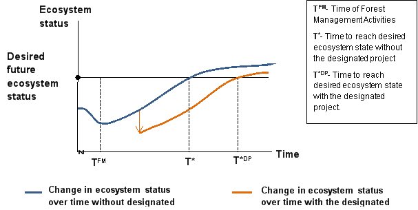
Example: Historical logging or mechanized forest resource harvesting may have progressively changed the status of an ecosystem in the past. These changes were then influenced by forest management activities aimed at reversing some of the effects (initiated at TFM in Figure 3).
Where a project is proposed in such an area, the future duration of the environmental effects of the project, in combination with those related to forest management, can support the selection of an appropriate future temporal boundary. This boundary would be set as the point in time in the future when the ecosystem can be restored to a certain condition or status.
As shown graphically in a simplified depiction in Figure 3, the desired future ecosystem state would have been reached at T* if the project had not been proposed. However, if the project goes ahead, the adverse environmental effects lead to a delay in when the ecosystem can reach the desired state. This occurs at T*DP, and could serve as the future temporal boundary for VCs within the ecosystem. Where data are available, the setting of past temporal boundaries can also be informed by knowledge of the ecosystem state at specific points in time.
Monitoring of the state of an ecosystem can be done over time using one or more indices (an index is an aggregation of measurable variables, see Appendix 3). For example, the measured variable can be associated with a key indicator species, such as a bird species known to be representative of the state of that particular forest ecosystem.
Level of Effort for Setting Temporal Boundaries
Spatial and temporal boundaries are set in light of other elements of scoping, including an understanding of how physical activities had, continue to, or will have an environmental effect on VCs.
The environmental effects of a physical activity on a VC must occur within the spatial and temporal boundaries set for the cumulative effects assessment (using the approaches outlined in this guidance) in order for that physical activity and its environmental effects to be considered in the cumulative effects assessment.
In addition to the overall level-of-effort considerations in the OPS (see Section 1.0 of this document for OPS level-of-effort considerations), the level of effort needed to establish temporal boundaries will vary with the:
- nature of the residual environmental effects, in terms of their measurability and scale or magnitude;
- time horizon of residual environmental effects of the project;
- time horizon of residual environmental effects of other past, present, and future physical activities; and
- selected temporal resolution(s) (i.e., years or decades).
Outcome Documentation
The outcome of this scoping element should be clear, well-supported documentation of:
- the methodologies and considerations used in the determination of temporal boundaries, including descriptions and rationale for scenarios if this approach is taken;
- the chosen past temporal boundary for the consideration of cumulative effects for each VC;
- the future temporal boundary for the cumulative effects assessment for each VC; and
- how the chosen temporal boundaries will adequately capture the expected cumulative effects.
The outcome documentation should be commensurate with the level of effort established. The documentation could involve a narrative description of each determined temporal boundary, or a table listing the VC with its chosen temporal boundary, accompanied by explanatory text.
1.4 Examining Physical Activities that have been and will be carried out
Physical activities to be considered in a cumulative effects assessment are not restricted to those listed in the Regulations Designating Physical Activities and those designated in an order made by the Minister of the Environment under subsection 14(2) of CEAA 2012.
Examining physical activities that have been and will be carried out is done as part of the scoping step (see Figure 2). The four elements of scoping are complementary, allowing for the results of each to inform integrated decision-making.
Examples of physical activities are numerous, and include agricultural development, management of a forested area, dredging a water body, hunting, fishing, remediation of a brownfield site, construction of a pulp mill, or operation and decommissioning of a mine. Practitioners should keep in mind that predicting cumulative effects to a VC will tend to be more accurate when all sources of environmental effects to that VC have been reasonably considered.
OPS Approach
The cumulative environmental effects assessment must consider other physical activities that have been carried out up to the time of the analysis, or will be carried out in the future, provided that these physical activities are likely to have an environmental effect on the same VCs that would be affected by residual environmental effects of the designated project.
Methodologies
1. Identifying Future Physical Activities
The OPS sets the methodology to be used for identifying future physical activities, by indicating that they are to be included in the cumulative effects assessment if they are certain and should generally be included if they are reasonably foreseeable. Some doubt about whether the physical activity will proceed is acceptable. The level of certainty may not be as high as for the project itself.
OPS Approach
A cumulative environmental effects assessment of a designated project must include future physical activities that are certain and should generally include physical activities that are reasonably foreseeable.
A future physical activity would be considered certain to proceed, and would be included in a cumulative effects assessment if one or more of the following criteria are met:
- The physical activity has received approval in whole or in part, such as:
- environmental assessment approval;
- pre-development approval for early works, permits for exploration, or collection of baseline data; or
- some other regulatory approval from a province.
- The physical activity is under construction;
- The site preparation is being undertaken.
A future physical activity could be considered reasonably foreseeable and should generally be included in the cumulative effects assessment if one or more of the following criteria are met:
- The intent to proceed is officially announced by a proponent. This information could be found in news media, the proponent’s website or via an announcement from the proponent directly to regulatory agencies.
- The physical activity is under regulatory review (i.e., the application is in process). This can be known, for example, if information about the review or application is available on a government website, or an EA notice has been made public.
- The submission for regulatory review is imminent. This could be known if the collection of data has already commenced, regulatory authorities have been contacted about information requirements, or through an announcement from the proponent.
- The physical activity is identified in a publically available development plan that is approved or for which approval is anticipated (e.g., a wastewater treatment plant in a city’s long term development plan).
- The physical activity supports – or is consistent with – the long-term economic or financial assumptions and engineering assumptions made for the project’s planning purposes.
- A physical activity is required in order for the project to proceed (e.g., rail or port transportation facilities, or a transmission line).
- The economic feasibility of the project is contingent upon the future development.
- The completion of the project would facilitate or enable the future development.
The criteria in the last three preceding bullets often relate to what is described as “induced development”. If the induced development is certain or reasonably foreseeable, it should be considered in the cumulative effects assessment. Examples of induced development include housing development that could arise due to the approval of the project.
OPS Approach
Here is how the concepts of ‘certain’ and ‘reasonably foreseeable’ are defined:
- Certain: the physical activity will proceed or there is a high probability that the physical activity will proceed, e.g. the proponent has received the necessary authorizations or is in the process of obtaining those authorizations.
- Reasonably Foreseeable: the physical activity is expected to proceed, e.g. the proponent has publicly disclosed its intention to seek the necessary EA or other authorizations to proceed.
2. Identifying Past and Existing Physical Activities
The following methodological options, or a combination of them, should be used to determine which past and existing physical activities to include in the cumulative effects assessment.
a) Using direct evidence relating to past and existing physical activities with VCs
Reasonable effort should be made to identify past and existing physical activities based on direct evidence available from the historical record and other reliable sources, such as reports, community knowledge or ATK.
OPS Approach
Present-day environmental conditions reflect the cumulative environmental effects of many past and existing physical activities.
Data and information on physical activities that occurred in the distant past is often limited. The challenge generally increases as the study extends into the past. In such circumstances, the information may still provide some insight into VC response.
Example: It may be known that early settlers cleared land for agriculture in the 19th century but then gradually abandoned part of the land due to changing lifestyles, or due to other factors such as declining fertility or drought. The abandoned portion of land may have naturally regenerated to its current condition of a forest or prairie. The available information may be anecdotal, but can still provide a defensible understanding of the environmental effects of agriculture, and informs the predictions of VC response to removal of the stressors.
Data and information on existing physical activities, or those that occurred in the recent past, are much easier to find. Sources include recent EA reports and land-use planning documents.
Example: A new coal mine is proposed in a watershed where there is an existing coal mine that releases selenium in the water that could potentially lead to cumulative effects on fish and fish habitat. The environmental effects of the existing mine in relation to fish and fish habitat must be understood in order to assess the cumulative effects of the new mine in the same region. Furthermore, any other past physical activity that has affected the watershed in relation to fish and fish habitat should be included.
In some cases, information on past or existing physical activities may help identify appropriate mitigation measures. Information on existing physical activities should cover their full lifecycle, particularly if decommissioning is certain or reasonably foreseeable.
b) Using present-day VC conditions to represent past and existing physical activities
This approach is used to address past and existing physical activities when a practitioner has only limited data and information, and needs a reliable means of making inferences about their effects on VCs. For example, it may be well-known that the current environmental conditions in a forested area exist in response to forest resource harvesting dating back to a distant past, but information on how the harvesting occurred and its effects over time may no longer be available.
In using this option, the practitioner first needs to consider whether the observed present-day VC conditions are indeed representative of the environmental effects of past and existing physical activities in the study area. Efforts are then focused on describing how past and existing activities may have contributed to the current state of VCs.
The practitioner should also attempt to evaluate whether the current VC condition is stable or whether it is still changing in response to past and existing physical activities. For example, an understanding of recovery stages after clear-cuts in similar environments may be helpful in determining whether the present-day VC condition is likely to remain stable or what its future state might be. This helps establish if present-day VC conditions are adequate surrogates for representing past and existing physical activities.
3. Any other option
If any other option is selected to identify past, existing, or future physical activities, it should be fully justified in the context of the project. It must also take into account the OPS, and enable the completion of an environmental impact statement that meets the information requirements of the project-specific EIS Guidelines and the legal requirements of CEAA 2012. Discussion with Agency staff prior to carrying forward any other option is recommended.
Considerations
Practitioners should take into account the following considerations in deciding which physical activities to include.
1. Appropriate information to gather about physical activities
As a general rule, the amount of information that can be obtained for future physical activity is usually proportional to the degree of certainty about it proceeding. For a past activity, there is generally more information available for projects that occurred in the recent past.
Each physical activity that is examined should be described in adequate detail to allow potential environmental effects to be characterized for later assessment. Key pieces of information to note about other physical activities may include:
- location, physical size (e.g., area covered, volume of process throughput), and spatial distribution of components (i.e., site specific, randomly dispersed, travel corridors);
- components (e.g., main plant, access roads, waste disposal site) and supporting infrastructure (e.g., waste treatment, power lines);
- expected life or period of activity (including start date), and phasing involved (e.g., exploration, construction, standard operations, later plans for upgraded or expanded operations, decommissioning, and abandonment);
- variations in seasonal operation (e.g., winter closures);
- frequency of use (for intermittent activities – e.g., helicopter use);
- transportation routes and mode of transport (e.g., roads, railways, shipping lanes);
- processes used (for industrial activity – e.g., open pit mining);
- emissions, discharges, and wastes that are likely to be released, and where;
- approvals received (e.g., permit and license conditions in effect); and
- duration of any in-place or planned follow-up program.
Where a scenario of future development is being employed, data surrogates for key pieces of information may be established by referencing typical development characteristics.
2. Information constraints
Information about a physical activity may not be readily available if, for example:
- proprietary technology or confidential production records are involved; or
- the design of the physical activity is too preliminary to provide enough useful information.
Information from similar physical activities at other locations (known as surrogate information) may be useful. It could be used in a case where future physical activities are reasonably foreseeable, but there is little information available.
Example: The development of a future gold mine may be considered reasonably foreseeable, but little information is available. Information on the environmental effects of a surrogate mine could be used. For example, the physical activity would probably include an open pit, mill, tailings storage facility, and water treatment facility. Caution in the use of this surrogate information would be required since the mine in question may have different geology or chemistry, processes, and tailings-management issues.
3. Pathways and categories of environmental effects
Pathway diagrams may assist in identifying and assessing environmental effects of other physical activities on the VCs identified (see Appendix 1: Source-pathway-receptor model).
The use of broad categories to assess physical activities in a generic way may be appropriate, for example, when little detail is available beyond the type of physical activities (e.g., forest resources harvesting), or when there are too many physical activities (e.g., in an urban area or along a highway) to characterize individually. Categories may be established in recognition of the similar patterns in the environmental effects they may cause. Examples include:
- shape (e.g., linear, aerially dispersed, areal point);
- sector type (e.g., resource extraction, power generation, urban infrastructure);
- industry type (e.g., mining, forest resource harvesting, municipal infrastructure); or
- transportation type (e.g., aircraft, boats, road traffic).
This information will be helpful when conducting the Step 2 analysis described in this document.
Level of Effort for Examining other Physical Activities
Spatial and temporal boundaries are set in light of other elements of scoping, including an understanding of how physical activities had, continue to, or will have an environmental effect on VCs.
The environmental effects of a physical activity on a VC must occur within the spatial and temporal boundaries set for the cumulative effects assessment (using the approaches outlined in this guidance) in order for that physical activity and its environmental effects to be considered in the cumulative effects assessment.
In addition to the level-of-effort considerations outlined in the OPS (see Section 1.0 of this document for OPS level-of-effort considerations), the level of effort needed to identify past, present, and future physical activities will vary with the:
- number of VCs under consideration;
- spatial boundaries selected;
- temporal boundaries selected;
- number of potential physical activities (past, present and future);
- land-use planning and/or applicable management plan information available;
- sensitivity of VCs to the perturbations of various physical activities;
- status of developments; and
- environmental and regulatory review applications for physical activities.
Outcome Documentation
The outcome of this scoping element should be clear, well-supported documentation of the:
- methodology used in the selection of physical activities;
- physical activities considered for inclusion which may include a map depicting the location of the physical activities in relation to the project and the VC under consideration; and
- physical activities considered for inclusion that will not be carried forward for analyzing cumulative effects.
A table or matrix format (as shown in Figure 4 below) may be useful for presenting information regarding the rationale for including each physical activity identified and the VCs that they may affect. It may also be used to categorize physical activities as past, existing, or future (certain or reasonably foreseeable). Where there is evidence that certain or reasonably foreseeable physical activities can be seen as induced development, it should be noted. Where scenarios are used to reflect future or past activities, it should also be noted.
The outcome documentation should be commensurate with the level of effort established. For example, in identifying past physical activities, the availability and use of an extensive historical record would require more documentation than in the case of a more limited historical record.
Past, Existing, and Future Physical Activities in a Largely Undeveloped Area |
Valued Components |
||||
|---|---|---|---|---|---|
1 |
2 |
3 |
4 |
Description |
|
Physical Activity A |
Check | Check | This future physical activity is reasonably foreseeable, since it is currently under regulatory review. It has the potential of affecting VC#1 & VC#2, given the nature of the physical activity and predicted effects pathways within the spatial boundaries established for these VCs. Furthermore, such effects on VC#1 & VC#2 are likely to occur within the same timeframe as the potential effects of the project on the same VCs. The effects of Physical Activity A and those of the project therefore both fall within the established temporal boundaries for VC#1 and VC#2. The environmental effects of Physical Activity A on these two VCs will be considered further in the Step 2 analysis. |
||
Physical Activity B |
Check | Check | Check | This is a past activity that will yield useful information about potential future effects on VC#1, VC#2 and VC#3. |
|
Physical Activity C |
Check | Check | This is a certain future physical activity with potential effects on VC#3 and VC#4. In the context of the area, it can be considered induced development. |
||
Physical Activity X |
This activity is not expected to affect any of the VCs identified for the cumulative effects assessment, therefore it is not included. |
||||
2.0 Overview and Outcomes of the Analysis
Step 2 of the framework is analysis of cumulative effects (see Figure 1).
This step builds on the results of scoping (Step 1) and considers how all physical activities identified during the scoping stage may affect the VCs within the spatial and temporal boundaries determined for the assessment of cumulative effects.
Step 2 analysis focuses on understanding the cumulative effects for each VC retained for further analysis.
OPS Approach
The methodologies used to predict cumulative environmental effects must be clearly described. With this information, reviewers of the EIS will be able to examine how the analysis was conducted and what rationale supports the conclusions reached. Any assumptions or conclusions based on professional judgment should be clearly identified and described.
Methodologies
Assessment of cumulative effects requires an understanding of both the estimated cumulative effects on VCs and the contribution of the project to cumulative effects.
The source-pathway-receptor model (see Appendix 1: Source-pathway-receptor model) can be used to depict the relationship between the project and other physical activities (as sources of an environmental change) and the VC (as the receptor affected by the change).
Baseline information serves as a point of reference – before a project is developed – against which cumulative effects can be predicted and assessed. In order to analyze cumulative effects, it is essential to understand the state of the receiving environment into which a project is entering. This means that, for each selected VC subject to analysis, information should be gathered on its state within the determined spatial and temporal boundaries.
One of the following options, or a combination of them, can be adopted to analyze cumulative effects on each VC.
1. Comparison using reference case(s)
Data from other areas with comparable conditions, or from a reference case, can be used to analyze or understand potential cumulative effects. Comparable conditions can include similar environments, or environments that are experiencing similar environmental effects as a result of similar physical activities. Some past physical activities may be included as a reference because they provide the best source of information for understanding past environmental conditions.
Example: An open pit metal mine in an area of boreal forest with many fish bearing streams could be a reference case for an open pit mine in a similar environment in a different part of the country.
The results of monitoring and follow-up of other similar physical activities that have similar receiving environments can be one source of information. This method is useful only when the reference case is comparable. The EA should include a rationale for the use of a reference case and explain its relevance, limitations, and assumptions for assessing the cumulative effects of the project.
When considering use of a reference case for a VC related to Aboriginal peoples as per section 5 (1)(c) of CEAA 2012, it is important to recognize that each Aboriginal group is unique and there may be specific considerations not addressed by the reference case.
2. Comparison using models
Predictive models can generate information that supplements available data or simulates existing and future conditions in those cases where data are limited or difficult to attain. Models can also estimate the response of a VC to cumulative effects.
Models can be qualitative (e.g., a conceptual model, typically less data-intense) or quantitative (e.g., a numerical model, typically more data-intense). The most common use of quantitative models is to predict the state of a physical condition or chemical constituent by using a computer-based application to assess various indicators or parameters such as air and water quality, species condition or response, water volume flows, airborne deposition on soils and vegetation, and habitat condition. Qualitative models can include descriptive narratives or graphic representations that illustrate the conceptual relationships between the environment and human activities.
Example: To model changes to groundwater flow linked to a Navigation Protection Act authorization (for the dewatering of a navigable water that would lead to changes in groundwater flow) under section 5 (2) of CEAA 2012, two types of models may be considered. A conceptual model would illustrate how groundwater flow may be affected by a project and other physical activities. A computer simulation of groundwater flow may predict the potential numerical quantity and quality of groundwater under a range of future conditions (e.g., future phases of the project or different mitigation measures), with or without the project.
Where models are used, it is necessary to provide the rationale for the chosen methodology, the assumptions involved in its use, and the limitations of the predicted data, including uncertainty on data interpretation, and statistical error and confidence.
3. Any other option
If any other option is selected, it should be fully justified in the context of the project. It must also take into account the OPS, and enable the completion of an EIS that meets the information requirements of the project-specific EIS Guidelines and the legal requirements of CEAA 2012. Discussion with Agency staff prior to carrying forward any other option is recommended.
Considerations
Practitioners should take into account the following considerations in conducting the analysis.
Environmental effects of other physical activities can interact with those of the project in various ways. For example, some effects may be simply additive, while others may result in effects greater than if they had occurred on their own (for more information, see Appendix 2: Types of Cumulative Effects).
Changes in the state of a VC may therefore be attributable to different changes to the environment resulting from the project and other physical activities that are acting together on the VC in various ways. In considering how various physical activities may interact to affect a VC, practitioners may find it helpful to compare the predicted future environmental state of the VC, both with and without the project.
The methodologies describe general ways that cumulative effects can be analyzed. Regardless of the methodology, a range of methods can be used. For more information about the types of methods that can be used, see Appendix 3: Methods for Cumulative Effects Assessment
Level of Effort for the Analysis
In addition to the overall level-of-effort considerations outlined in the OPS (see Section 1.0 of this document for OPS level-of-effort considerations), the level of effort needed to undertake the analysis of cumulative effects will vary depending on the:
- sensitivity of the VC to the environmental effects of the project;
- likely contribution of the project to cumulative effects;
- complexity of a VC’s response to multiple environmental stressors;
- state (health, status, or condition) of a VC with regard to known thresholds, standards or benchmarks;
- past or existing disturbance levels and extent of other physical activities that are or may contribute to cumulative effects on the VC; and
- selected methods used for the assessment.
Outcome Documentation
The outcome of the analysis should be a clear, well-supported documentation of the:
- methodological approach and methods used and the rationale for their use;
- estimated cumulative effects on VCs resulting from the project in combination with the environmental effects of other physical activities that have been or will be carried out, including the analysis conducted and rationale supporting the conclusions reached; and
- contribution of the project to the cumulative effects, considering past, existing, and future physical activities, to facilitate the identification of appropriate mitigation.
The outcome documentation should be commensurate with the level of effort established. Outcome documentation may include VC specific descriptions of the methods used to analyze each VC and the results of analysis. The level of detail contained in each respective section should be consistent with the level of effort required to analyze the corresponding VC.
2.1 Analyzing Various Types of Data and Information
Having access to data and information related to other physical activities and traditional and community knowledge is critical for conducting the Step 2 analysis.
To make decisions about which data is to be collected or generated, practitioners should have a clear understanding of how the data and information will be used in the assessment, how to establish a proper scale of analysis, and what methodologies and specific methods will be employed for their analysis.
OPS Approach
Data collection and/or generation are important components of a cumulative environmental effects assessment. At times, it may be challenging to obtain or generate data to support the analysis.
Methodologies
The methodological options presented here orient the analysis of various types of data and information frequently used in a cumulative effects assessment.
1. Using information about current and past environmental conditions
OPS Approach
A description of past environmental conditions can improve the understanding of cumulative environmental effects for a specific VC.
The OPS recognizes that a description of past environmental conditions can improve the understanding of cumulative effects for a specific VC. As such, practitioners should make reasonable efforts to understand the extent to which past and present physical activities are responsible for baseline conditions.
Baseline data can be compared to past conditions to reveal spatial or temporal patterns or trends so that predictions can be made. Information on past environmental conditions may also help establish if present-day VC conditions are likely to be stable. For example, data and information on the response of a forested area to harvesting over time may help establish if the current state has reached equilibrium and/or if the response over time corresponds to the body of knowledge on recovery stages.
Some characteristics of useful baseline information for the purpose of a cumulative effects assessment under CEAA 2012 include:
- detailed data (either qualitative or quantitative) are available for each selected VC within the spatial and temporal boundaries identified for the cumulative effects assessment;
- natural variability, drivers of change, and historical shifts for the VC are identified, if reasonably obtainable;
- trends or spatial patterns in quality, quantity, value, or use of VCs are identified where reasonably obtainable;
- the current status of the existing environment is presented in the context of relevant benchmarks; and
- data or perspectives relevant to baseline conditions include those that are obtained through community knowledge and/or ATK, where appropriate.
Models may be used to generate baseline conditions. For more information on conceptual and numerical models, see Appendix 3.
2. Using information on the environmental effects of physical activities
OPS Approach
Information on the environmental effects of past or existing physical activities may be helpful:
- if the effects of past or existing physical activities on a specific VC will help predict the environmental effects of a designated project;
- if information on past or existing physical activities will assist in the identification of appropriate mitigation measures for the designated project; or
- if an existing physical activity will be decommissioned in the future and this decommissioning would affect the future condition of a specific VC.
The focus of a cumulative effects assessment is on understanding key environmental effects on specific VCs in conjunction with other past, present and reasonably foreseeable physical activities.
Pathway diagrams are useful to identify and evaluate potential cumulative effects on VCs by exploring linkages to other physical activities (see Appendix 1 for more information).
However, as a region becomes more heavily disturbed due to increasing development, it may become difficult and less relevant to determine which physical activity is contributing to specific environmental effects, and to what degree. While attributing specific environmental effects to individual physical activities may not always be feasible, estimation of the cumulative effects on VCs should be done.
It is important to consider if past physical activities that are no longer physically present, operating, or active continue to affect an identified VC (e.g., ongoing environmental effects of an abandoned gravel pit, or a contaminant plume from a brownfield site). In some cases, the source and pathways of environmental effects may no longer be readily observable; however, they may continue to affect the state of the receptor VC. Consideration should also be given to whether an existing physical activity will be decommissioned in the future, and whether this decommissioning might affect the future condition of a specific VC.
If the state of the VC is likely to be stable, then the cumulative effects assessment can address how the baseline will be further affected by additional changes in the environment due to future activities. On the other hand, if the VC is still changing as a result of past or existing activities, then the analysis has to address two influences: i) how past and existing activities are expected to affect the future; and ii) how future activities will affect the future.
With complex interactions, the whole does not necessarily correspond to the sum of the parts. Continuing environmental changes associated with past and existing activities may result in a worsening or improvement of VC conditions. Where there is evidence that effects are not simply additive, it should be noted.
Example: The operation of a generating station releases cooling-water effluent into a lake that results in a change in the fish population due to thermal pollution. The fish population is also affected by fishing and sewage-related pollutants from residential development along the shoreline. All of these types of environmental effects on the fish should be included in the cumulative effects assessment.
3. Using Aboriginal traditional knowledge and community knowledge
OPS Approach
Community knowledge and ATK available to the proponent should be incorporated into the cumulative environmental effects assessment, in keeping with appropriate ethical standards and without breaking obligations of confidentiality, if any.
Collection and use of ATK is addressed in the reference guide Considering Aboriginal traditional knowledge in environmental assessments conducted under the Canadian Environmental Assessment Act, 2012.
How community knowledge and ATK available to the proponent are used for the assessment of cumulative effects should be described and be a part of the selected methodological approach, without breaking obligations of confidentiality, if any, while also maintaining appropriate ethical standards. Legislated requirements associated with access to information must be considered.
Considerations
1. Establishing the proper scale for analysis
The assessment area for cumulative effects may be larger than required for the assessment of the project-related environmental effects to capture the greater extent of overlapping cumulative effects of other physical activities. The type of data required may change as the scale of the assessment changes.
Where cumulative effects extend over larger areas, the assessment may have to be based on satellite imagery or existing habitat surveys completed at very broad scales.
Example: Maps or photo mosaics at scales ranging from 1:250,000 to 1:50,000 are sometimes used to depict broad-level baseline environmental data for the purposes of a cumulative effects assessment (e.g., to convey available habitat). In some cases, it may be more instructive to include photos of the area (regular or panoramic views) and surrounding areas rather than maps (e.g., to depict changes in viewscape).
In other cases, practitioners may rely on various landscape-level metrics, such as linear feature density, as a predictor of the change in VC health, status, or condition, or to characterize the degree of disturbance or activity. Regardless, practitioners should select appropriate scales and tools to support meaningful evaluation.
In some cases, the scale is small and relies on field surveys.
Example: Species-at-risk studies may be relatively intensive within the proposed footprint of the project and involve on-site mapping.
2. Selecting the appropriate analytical method
Different methods can be used to analyse the data and information (see Appendix 3). Selecting the method to be used will depend on the nature of the data and information available and generated for the cumulative effects assessment, as well as the nature of the VC and pathways of effects.
Level of Effort and Types of Data and Information
In addition to the overall level-of-effort considerations outlined in previous sections of this document, the level of effort needed to undertake the analysis of cumulative effects will vary depending on the:
- quality/quantity of information collected about cumulative effects for each VC during the scoping process;
- quality/quantity of information available about the environmental effects of other physical activities that contribute to cumulative effects;
- amount of existing knowledge on a VC’s sensitivity to environmental effects (natural and anthropogenic); and
- amount of data judged useful for modelling, mapping, statistical analyses or any other methods used.
Outcome Documentation
EA documentation must clearly explain and justify the methodologies and methods that have been used to assess cumulative effects, along with the following supporting information:
- types of data and information that were gathered or generated for each VC, and why this information was deemed necessary ;
- specific methods that were used to gather or generate this data and information, and why they were selected; and
- specific methods that were used to analyze this data and information, and why they were selected.
The outcome documentation should be commensurate with the level of effort established. For example, the amount of existing data used in the analysis versus the generation of new data will vary according to project-specific variables. Concerns of Indigenous groups regarding a specific aspect of a VC may necessitate the generation of new data through field studies. In this case, detail regarding the methods used in the study and any rationale for their selection should be documented.
2.2 Addressing Data Limitations and Uncertainty in the Analysis
Collecting and using appropriate data and information is central to the analysis of cumulative effects. A reasonable attempt to collect data and information must be demonstrated. A lack of reliable data and information will tend to make the predictions less certain, and potentially faulty.
Few – if any – cumulative effects predictions are certain. Uncertainties associated with information and methods may occur at many points in the process of analyzing cumulative effects. For example, there may be poor information about other physical activities, or conflicting reports about the effectiveness of mitigation measures. Even where the data are reliable, data interpretation could be challenging. For example, it may not be clear to what extent an effect pathway is likely to result in a change in the environment.
Practitioners must meet the requirement to assess cumulative effects in the face of data limitations and uncertainty. The EIS should present a complete picture of the potential types and scale of cumulative effects and the data required and used for their assessment. While there are frequent data limitations in cumulative effects assessment that cannot be fully overcome, the uncertainties that result from these limitations should be documented.
Assumptions used in modelling and other analytical methods may limit the analysis. Where possible, it should be noted if results are sensitive to small changes in assumptions
OPS Approach
Potential cumulative environmental effects should be considered, as appropriate, in the analysis, even when there is little supporting data or there is predictive uncertainty.
Reviewers of the EIS should be presented with a complete picture of the potential types and scale of cumulative environmental effects. In all cases, uncertainties and assumptions underpinning an analysis should be described and information sources clearly documented.
Methodologies
Various methodologies used to address data limitations and uncertainties in a project EA are also useful in considering cumulative effects.
1. Documenting efforts and limitations
A reasonable attempt to collect and/or generate information must be demonstrated. A lack of usable information for the analysis can have important implications to the predictive certainty of the cumulative effects assessment.
Where there is little supporting data, or where there is predictive uncertainty, the assessment of cumulative effects should still be conducted.
Limitations imposed by data and other types of uncertainty should be clearly described. This involves outlining how these limitations affected the choice of methodology and assumptions.
2. Using various sources and types of knowledge
A variety of approaches for addressing data limitations are available and have been mentioned in other parts of this technical guidance, including:
- use of ATK and community knowledge to fill data gaps;
- use of surrogate data from similar areas to estimate past environmental conditions;
- use of surrogate data from similar physical activities to predict cumulative effects;
- modelling to assess possible cumulative effects over the range of future conditions; and
- inferences based on an appropriate body of knowledge, using professional judgment.
3. Using scenario building
Scenario building may be useful to account for a range of future conditions for a VC and address uncertainty regarding the future state of a VC.
Scenario building consists of describing a set of possible alternatives that might reasonably take place leading to several possible past or future conditions. They are most helpful for studies of the mid- and long-range future and when several alternative scenarios – each one significantly different from the others – are to be considered.
4. Using adaptive management
Adaptive management may be an appropriate strategy for helping to reduce uncertainty about the environmental effects and the effectiveness of mitigation. Adaptive management provides flexibility to identify and implement new mitigation measures or to modify existing ones during the life of a project.
However, a commitment to implementing adaptive management measures does not eliminate the need for sufficient information regarding the cumulative effects of the project, the significance of those effects, and the appropriate mitigation measures required to eliminate, reduce or control those effects.
For further information on adaptive management, see the Agency’s Operational Policy Statement: Adaptive Management Measures under the Canadian Environmental Assessment Act, or any future updates to that document.
Considerations
Although aspects of cumulative effects cannot be known with certainty, that does not mean the EA is deficient. The practitioner must simply strive to provide the best information to support decisions about the project.
In determining whether data and information should be obtained or generated, practitioners should consider the ability, cost, and utility of the data to be collected, its intended use, and the limitations to its use in the assessment of cumulative effects. This also needs to be weighed against the nature and scale of the project, the receiving environment and the potential cumulative effects.
Caution should be exercised if the degree of uncertainty is unusually large (e.g., effects are expected in the future, but it is not possible to predict whether they will improve or harm a particular VC). In these cases, predictions will be highly sensitive to the assumptions made. Relying on a particular assumption could result in a faulty conclusion. It would therefore be appropriate to present the results as a range, in line with the range of underlying assumptions.
In addition, as set out in the OPS, a Step 5 follow-up program can be established to monitor the VC. This will help determine whether the mitigation measures identified in Step 3 are appropriate in the face of actual environmental effects.
Level of Effort to Address Uncertainties
The level of effort needed to address uncertainty will depend on:
- what decisions were made in Steps 1 and 2 concerning VCs, methodologies, methods, and data collection; and
- what is required to clearly state assumptions and data limitations throughout the EA.
Outcome Documentation
In addition to the criteria identified in previous subsections on analysis, the outcome of the discussion of data limitations and uncertainties should be a clear, well-supported documentation of:
- model assumptions and data limitations in the assessment of cumulative effects; and
- the implications of assumptions used and their limitations for the predictive certainty of the cumulative effects assessment.
The outcome documentation should be commensurate with the level of effort established. For example, the number and complexity of any model assumptions and data limitations will affect the documentation needed to explain the implications of the assumptions and data limitations.
Appendix 1: Source-pathway-receptor Model
This Appendix provides information on the source-pathway-receptor model as background information. This model (see Figure 5) is used in EAs to identify:
The source of an environmental change (source)
The source is the activity or event that causes environmental stresses. For example, the source might be the project (i.e., a mine) or another physical activity (i.e., agriculture).
What the source may affect (receptor)
The receptor is the environmental component that is affected by the impacts of a physical activity. Since receptors differ in health and resiliency, each receptor has its own, unique sensitivity to environmental change. These receptors are the focus of the cumulative effects assessment and are typically referred to as VCs.
How the source may reach the receptor (pathway)
The pathway is the route the source takes to reach a VC. Pathways are the mechanisms through which a change in the environment occurs. Pathways can include physical or chemical transport through air, water, soil, animals, food supplies, etc. In order to consider cumulative effects, it is essential to understand these mechanisms and the state of the receiving environment within which a project takes place.
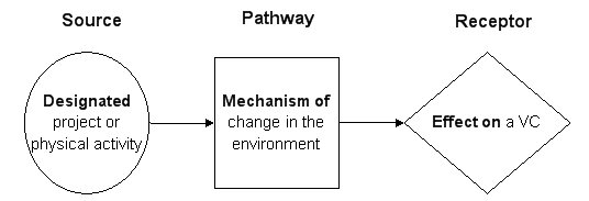
Appendix 2: Types of Cumulative Effects
This Appendix provides information on types of cumulative effects.
It is important to consider how cumulative effects may interact and manifest in practice in order to make sound and justifiable predictions about their significance. Key types of cumulative effects presented in this reference document include:
- additive;
- synergistic;
- compensatory; and
- masking.
Determining how cumulative effects occur can be a complex task, and can vary based on the VC being assessed. For example, even if the cumulative effects on habitat are additive, the ultimate effect on a species may be synergistic. Although classifying cumulative effects can be helpful to conceptualize various forms of cumulative effects, the critical point is the need to assess how the cumulative effects are acting on VCs (Duinker & Grieg 2006).
Additive Cumulative Effects
An additive cumulative effect is the sum of individual effects of two or more physical activities. Figure 6 demonstrates the loss of habitat increases with each new element of development (a new town, followed by new roads and a golf course).
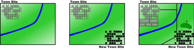
Synergistic cumulative effects
A synergistic cumulative effect occurs as a result of the interaction between two or more effects, when the resultant combination is greater or different than the simple addition of the effects. Consider the example described in the following text and shown in Figure 7 (adapted from Greig, L.A. et al, 2003).
Panel A: Caribou habitat is divided in two large blocks joined by a migration corridor. Each block has contiguous winter and summer habitats, but their proportions are unequal and reversed in the two blocks.
Panel B: Harvest of timber is assumed to remove the small southern areas of winter and summer habitats with relatively little effect on carrying capacity for the migratory caribou herd.
Panel C: Harvest of timber in the migration corridor is assumed to almost completely block migration. Animals stranded in one or the other large habitat block need to find life requisites for the entire year in that block by utilizing the smaller habitat blocks, and the carrying capacity is substantially reduced.
Panel D: The synergistic cumulative effects of both projects combined is expected to reduce the caribou carrying capacity of the total area much more than the sum of the carrying capacity reductions of the two actions when taken independent of each other.
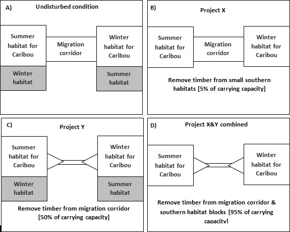
Compensatory Cumulative Effects
Compensatory cumulative effects are effects from two or more physical activities that “offset” each other.
For example, as illustrated in Figure 8, a metal mine project might cause a decrease in a specific fish population due to effluent discharges, while a cogeneration plant might enable an increase in this same population through its warm water discharges. These effects may offset each other and, accordingly, the cumulative effects on this fish population may not be measureable.
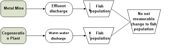
Masking Cumulative Effects
The effects of one project might mask the effects of another in the field. For example, as illustrated in Figure 9, the warm water plume associated with a generating station (shown under “A” in Figure 9) may be of such magnitude that the effects of a small plume associated with another project (introduced as shown under “B” in Figure 9) would not be detected. If the generating station were to stop its physical activities, then the effect of the other project would become visible.
It is therefore possible that the effects of an earlier project could mask the effects of a new project. In this case, it is reasonable to conclude that the new project is not likely to result in environmental effects. This conclusion is correct as long as the effect of the earlier project continues. Once this earlier project is terminated, the effect from the new project would become evident. If masking of cumulative effects is predicted, a follow-up program may be required to ensure that mitigation measures remain effective in managing cumulative effects when the earlier project is terminated.
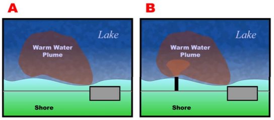
References
Gartner Lee Ltd. 2006. Cumulative Effects Assessment “Tips” Document. Prepared for the Canadian Environmental Assessment Agency.
Greig, L. A., P. N. Duinker, R. R. Everitt, and K. Pawley. (2003). Scoping for cumulative effects assessment. Prepared for Indian and Northern Affairs Canada Environment Directorate, Whitehorse, Yukon Territory. ESSA Technologies Ltd., Richmond Hill, Ontario.
Duinker, P. N., & Greig, L. A. (2006). The impotence of cumulative effects assessment in Canada: ailments and ideas for redeployment. Environmental Management, 37(2), 153-161.
Appendix 3: Methods for Cumulative Effects Assessment
This Appendix provides a brief introduction to some of the methods that may be used in the cumulative effects assessment for Step 1 (scoping) or Step 2 (analysis).
Numerous methods are available for conducting a cumulative effects assessment, and often these are simply typical EA tools modified to better consider cumulative effects. The methods discussed in this Appendix include:
- Questionnaires and Interviews;
- Checklists and Matrices;
- Network and Systems Analysis/Diagrams;
- Indicators and Indices;
- Conceptual and Numerical Models;
- Trend Analysis; and
- Spatial Analysis.
Questionnaires and Interviews
Description
Questionnaires and interviews are a means of gathering a broad range of information from knowledgeable or interested individuals or groups.
These methods can be used to collect information about past, present, or planned development projects, baseline data, changes in the socio-economic environment over a period of time, and opinions about where, why, and how cumulative effects may occur.
Applicability to Cumulative Effects Assessment
Interviews and questionnaires can be used to assist in the collection of baseline data and increase understanding of the environmental effects of other physical activities, the VCs affected, and possible mitigation measures. Interviews and questionnaires are most applicable to the scoping of the cumulative effects assessment.
It can be useful to interview experts during scoping and/or analysis to provide a range of expert knowledge during a cumulative effects assessment.
Checklists and Matrices
Description
A checklist is a simple method that can be used to record VCs and potential cumulative effects, but is not typically useful for analysis.
Matrices can be used to summarize and present complex information in a concise manner. Matrices are two-dimensional grids, with information arranged in rows and columns. Practitioners can enter data in the form of descriptive words, symbols, or numbers into the grid to record and organize information. Matrices range from simple interaction matrices, with project physical activities along one axis and VCs along the other, to more complex matrices that describe potential cumulative effects. Matrices can also describe mitigation and follow-up relative to specific cumulative effects.
Applicability to Cumulative Effects Assessment
Checklists are most applicable to the scoping of the cumulative effects assessment to, for example, help highlight common or likely cumulative effects among physical activities and the project under consideration.
Matrices can be used to present and organize information on the cumulative effects of a project and other physical activities on VCs. They are often used to identify the likelihood of cumulative effects on one or more VCs. They can also be used to score or rank cumulative effects. Matrices are often used in EA reports to add information such as mitigation and follow-up recommendations, and even the significance of the cumulative effects and the contribution of the project.
Network and Systems Analysis/Diagrams
Description
Network and systems analysis identifies the pathway of cumulative effects using a series of chains or webs between a proposed action and a VC. This method is based on the concept that there are links and interactions between individual VCs. A VC is affected not only directly by the source activity, but also indirectly through another VC. This method uses a network or system diagram, which is essentially a flow chart with connector lines between a project and/or physical activities and VCs.
An example of a network or system diagram for cumulative effects assessment is provided in Figure 10.
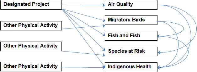
Applicability to Cumulative Effects Assessment
By mapping cause-and-effect relationships among projects, other physical activities, and VCs, possible cumulative effects can be identified. Network and systems analyses are most applicable to the scoping of the cumulative effects assessment, and can be helpful to identify the pathways among a project, multiple other physical activities, and multiple VCs.
Indicators and Indices
Description
In EA, an indicator is a measurable variable and an index is an aggregation of variables. Both can represent the state (health, status, or condition) of a VC. For example, if caribou are selected as a VC, then indicators might include the total size of the herd, the density of animals in a habitat, and rates of mortality and reproduction.
An indicator or index can represent environmental effects on more than one VC. For example, habitat fragmentation can be an indicator of habitat quality for wildlife or vegetation or the current use of lands and resources for traditional purposes by Aboriginal peoples.
a) Stress Indicators
Stress indicators are measurements that provide information about the attributes of human-caused disturbances or the surrounding environment, such as the magnitude, intensity, and frequency of physical activities, or natural phenomena that may bring about changes in environmental components. Some examples of stress indicators for which models have been developed and have been correlated to specific VC conditions include kilometres of roads per square kilometre; total cleared area; percent of area disturbed by class of activity; total area burned; and stream crossing density.
b) Ecological Indices
An ecological index is a numerical or descriptive categorization of a large quantity of ecological data or information involving multiple metrics. It is used to summarize and simplify information, to make it useful to decision-makers and stakeholders. Some examples of ecological indices are core habitat area, habitat patch size, index of biological integrity, and Hilsenhoff biotic index.
c) Social Indicators
Social indicators provide information on social VCs and facilitate comparisons over time that are well-suited for examining long-term trends in a community. Some examples of social indicators are population size and growth, equity (distribution of benefits), quality of life (self-assessed), locus of control (psychological), and cultural well-being.
Applicability to Cumulative Effects Assessment
Indicators and indices can be used during the scoping, analysis, significance, and follow-up steps of the cumulative effects assessment. For the determination of significance, indicators and indices can form the basis for establishing benchmarks. In cumulative effects assessment, indicators and indices can be useful for:
- summarizing and communicating information on the health, status, or condition of a VC, either in the present or historically;
- increasing the understanding of a VC’s response to environmental effects;
- acting as a tool for evaluating VC sustainability over time;
- evaluating the effectiveness of mitigation measures and cumulative effects management strategies; and
- planning follow-up, monitoring, and adaptive management programs.
Conceptual and Numerical Models
Description
Conceptual and numerical models are methods that represent or simulate the environmental interactions among projects, VCs, and other physical activities. Models used in cumulative effects assessment can be qualitative (conceptual models) or quantitative (numerical models).
a) Conceptual Models
Conceptual models are generalizations of reality that provide an understanding of a more complex process or system. They represent the relationships among receptors (e.g., VCs), stressors (e.g., environmental effects), and sources of stressors (e.g., projects or other physical activities). The outputs from conceptual models are typically qualitative or descriptive narratives, or graphic representations, such as a matrix or a box-and-arrow diagram.
Conceptual models may enhance understanding of the response of VCs to environmental effects resulting from past and existing physical activities. They may also serve as a useful tool to represent the structure, functions, and hierarchical relationships of the terrestrial, aquatic, and atmospheric systems affected by physical activities.
b) Numerical Models
Numerical models are a set of mathematical equations developed to simulate the behaviour of a system over time. They enable the quantification of cause-and-effect relationships by representing environmental conditions. A model could focus on a particular VC (e.g., water quality), or could represent a complex natural system. Some examples of commonly used numerical models are hydrological and hydrogeological models, air and water dispersion models, and species habitat models. In order to assess changes in the environment, such as air and water quality, water volume flows, and airborne deposition on soils and vegetation, numerical models usually require computers to provide solutions using complex and iterative numerical methods.
Modelling can be a powerful technique for quantifying the cause-and-effect relationships leading to cumulative effects. Once the linkages have been quantified, numerical models can be used to make predictions into the future.
Applicability to Cumulative Effects Assessment
In a cumulative effects assessment, models can be used to identify and provide:
- the characteristics and interactions between VCs, the project, and other physical activities;
- the anticipated cumulative effects of multiple physical activities or events within identified study spatial and temporal boundaries;
- linkages of processes and environmental effects across disciplinary boundaries; and
- a scientific basis for the identification of VCs and their associated indicators, the establishment of spatial and temporal boundaries, the identification of other physical activities, and the prediction of cumulative effects.
For example, the Impact Model approach involves testing the validity of a statement, similar to that made in a scientific hypothesis. Such hypotheses provide a clear basis for prediction of cumulative effects by setting out how cumulative effects are likely to arise, and the accompanying rationale for a prediction.
Trends Analysis
Description
Trends analysis assesses the health, condition, or status of VCs over time, and is commonly used to develop projections of past or future conditions. The trend is often described relative to an environmental benchmark. The objective of trends analysis is to identify a pattern – in the form of a mathematical equation – which represents the behaviour of a VC. To support trends analysis, the data can be depicted in various ways, including:
- a simple quantitative indicator of a trend, such as numbers of animals from annual surveys, to reflect changes in population levels over time;
- a series of figures illustrating changes in habitat pattern;
- video simulations from a modelling exercise, showing complex changes in geographic or aesthetic resources (i.e. visual landscape); and
- aerial imagery showing time-series information.
Applicability to Cumulative Effects Assessment
Trends can help practitioners identify cumulative effects issues, establish appropriate environmental baselines, or project future cumulative effects.
Spatial Analysis Using Geographic Information Systems
Description
Spatial analysis is a method for identifying the spatial distribution of effects or analyzing geographic information. Spatial analysis can be applied to a range of physical activities and environmental conditions, and is used for identifying physical effects in terms of geographical location. Geographic information systems (GIS) are the most commonly used tool in spatial analysis.
a) Geographic Information Systems
GIS typically involves the preparation of maps or layers of geographic information that are then superimposed on one another. The layered map can be used to provide a composite picture of the baseline environment .
With GIS it is possible to correlate measures of disturbance to physical activities and relate those disturbances to the occurrence of VCs. This is a tool for creating a model of cause-effect relationships.
b) Overlay Mapping
Overlays provide a technique for illustrating the geographical extent of different environmental effects. Each overlay can be a layer of information, such as a map of a single effect. When superimposed on one another, the overlaps illustrate areas where there are potential cumulative effects.
With GIS software, overlay mapping is particularly suitable for pinpointing sensitive zones where development should not occur. This can then serve as the basis for land management proposals and other mitigation measures.
Applicability to Cumulative Effects Assessment
Spatial analysis is useful for identifying where cumulative effects may occur as a result of the geographic location of the project in relation to other physical activities.
GIS is also a useful tool in cumulative effects assessment owing to its ability to store, manipulate, and display large sets of complex, geographically referenced data. It is well suited to complex spatial applications, and can be used to display the consequences of multiple actions and to support mitigation proposals for undertaking cumulative effects assessments.