
The ABC Method: a risk management approach to the preservation of cultural heritage
This manual offers a comprehensive understanding of risk management applied to the preservation of heritage assets, whether collections, buildings or sites. It provides a step-by-step procedure and a variety of tools to guide the heritage professional in applying the ABC method to their own context. The method can be applied to a range of situations, from analysis of a single risk to a comprehensive risk assessment of the entire heritage asset.
[PDF version, 2.45 MB]
Table of contents
- Overview
- Step 1: Establish the context
- Tasks for the establish the context step
- Explanations for the establish the context step
- Task scope and time horizon
- Mandate, policies, and procedures of the organization
- Legal context
- Financial context
- Governance context
- Stakeholders
- The value pie: Introduction
- The value pie: Setting up the table
- The value pie: Using value categories
- The value pie: When items aren’t so easily defined
- The value pie: Using values directly as intangible items
- The value pie: Multiple contributing values to each item
- Items with multiple values: A worked example
- The value pie: Capturing ensemble value
- The value pie: Applying it to only some parts of the heritage asset
- The value pie affects risk assessment
- Step 2: Identify risks
- Tasks for the identify risks step
- Explanations for the identify step
- Identify specific risks
- Write the risk summary sentences
- Susceptible and exposed = affected
- Checklists
- Frameworks and their purpose
- The 10 “Agents” of deterioration
- The causal chain from hazard to adverse effect, via the 10 agents
- The three “Types” of risk occurrence
- “Rare” as a rigorously defined term
- The five “Stages” of control
- The six “Layers” around the heritage asset
- The three sources of knowledge
- Comprehensive risk identification: The Ten Agents and Three Types of Occurrence Table
- Comprehensive risk identification: Use efficient paths for surveys
- Rare events and regional data
- Collecting local knowledge
- Identifying risks by causes other than the 10 agents
- Step 3: Analyze risks
- Tasks for the analyze step
- Explanations for the analyze step
- The three ABC components for quantification of risk
- The ABC scales
- A scale: Frequency or rate
- B scale: Loss of value to each affected item
- C scale: Items affected
- Do you want paper or electronic?
- The risk scenario
- Analyzing A for rare events
- Analyzing A for common events
- Analyzing A for cumulative processes
- Analyzing A using a time horizon
- Analyzing which items to include: Check the value pie for guidance
- Analyzing B when loss is total
- When loss is partial: Analysis of the deterioration
- When loss is partial: From deterioration to loss of value
- When loss is partial: Using fractions
- When loss is partial: Using diagrams
- When loss is partial: Using words
- When loss is partial: Using equivalence to total loss
- When loss is partial: Equivalence chains
- When loss is partial: Value judgements may not be necessary
- Analyzing C if all items have equal value
- Analyzing C when items vary in value
- Analyzing a risk by using the probable institutional response
- Review for coherence in the analysis of the three components
- Finding knowledge
- Knowledge phases during risk analysis
- Aggregating and disaggregating specific risks
- Facts plus theories: The general method for analyzing scenarios
- Theory: Exposure to events
- Theory: Exposure to cumulative processes
- Analyzing risks by control levels
- Can we predict the future?
- Making deductions from the evidence of past adverse effects
- Separating the technical issues from the subjective issues during the analyze step
- The arithmetic behind the ABC scores
- Step 4: Evaluate Risks
- Step 5: Treat Risks
- Conclusion
Overview
Introduction
The main lesson from these experiences has been that scientific expertise, rational decision making, and public values can be reconciled if there is a serious attempt to integrate them. The transformation of the risk arena into a cooperative risk discourse seems to be an essential and ultimately inevitable step to improve risk policies and risk management.
No one is distressed by failing to see very subtle points that require specialized knowledge. We are distressed, however, if we overlook the obvious.
Welcome to heritage risk management
Why use it?
If you have ever wondered what to do when facing a pressing and difficult preservation decision, then this method can help.
If you have ever wondered how to balance preservation with sustainability, shrinking resources, user demands, and public accountability, then this method can help. Finally, if you have ever wondered how to present all this succinctly to decision makers, with transparent priorities, then this method can help.
The goal of heritage risk management
In simple language, our goal is the best preservation of the value of the heritage asset with the available resources.
In more technical terms, our goal is to assess the risks and deterioration processes affecting our heritage asset, and then to act to reduce them as effectively as possible, given the available resources.
What is risk-based decision making?
Risk-based decision making is the application of risk assessments to a decision. The distinction with risk management is only a matter of degree. Many useful preservation decisions can be made using very focused assessments of one or two risks. If, on the other hand, one wants to “manage” risks of a heritage asset, one needs assessments of most, if not all, of the risks.
Structure of the manual
Overview section
The Overview section summarizes the who, what, why, and how of the method. Several examples of its use are provided. It opens the door to thinking about not only comprehensive risk management, but also smaller decisions within heritage preservation, i.e. risk-based decision making.
The five steps
The core of the manual is built around the five steps of a management cycle. These are:
- Establish the context
- Identify risks
- Analyze risks
- Evaluate risks
- Treat risks
Within each of the steps, the manual provides a subsection on tasks and a subsection of explanations.
Tasks
For each of the five steps, three or more tasks have been outlined. The sections on each step begin with these tasks. Each task is explained by a list of detailed activities.
Who can do this?
Anyone responsible for heritage preservation
This manual outlines the ideas behind risk management of heritage assets, such as collections, buildings, and sites, and provides a step-by-step procedure for doing it. Once you begin to view preservation decisions from this perspective, you will be “doing” heritage risk management.
A participatory process
Risk management involves many players inside and outside the organization. This manual can be used to inform all participants.
Just want the big picture?
For those just curious about the method, or who have been asked to participate in the process, please read the Overview section.
First-time user?
This manual was developed as a resource for a course in the method. The best way to use it is in the context of mentoring or training.
If you are trying to apply the full method for the first time, without the benefit of a teacher, we suggest that you begin by reading the entire manual. Then locate one of the many individuals around the world who have taken the ICCROM course called “Reducing Risks to Collections” (see the ICCROM website for lists of participants) and who are passionate about sharing and building the method. Canadians can contact CCI for assistance; others, please contact the organization ICCROM.
Paper method or database?
Paper
This method can be applied using only paper forms. Some calculations and graphing will be necessary. This can be managed with a calculator or by using spreadsheet software such as Microsoft Excel® or OpenOffice.
Database
The most convenient tool is the CCI Risk Management Database, developed specifically for the method. It automates all the calculations necessary for comprehensive assessments and the evaluation of risk reduction options. It generates reports based on your data and text entries. For information on the database, contact CCI.
Origins of the Manual
Partner Institutions
From 2006 until 2012, ICCROM, the Canadian Conservation Institute (CCI), and the Netherlands Cultural Heritage Agency (RCE; formerly the Institute for Cultural Heritage, ICN) established a collaboration framework “to create an international shift in attitude from traditional preventive conservation practice to risk management within the heritage profession.” Among the activities of this collaboration were research, training and dissemination, and the production of resource materials, which CCI was to lead.
Manual background
This manual was conceived in the framework of that collaboration. Since then, the text has been substantially revised based on the experience of CCI in applying the ABC method to Canadian institutions and that of ICCROM in projects carried out in Latin America, Asia, and Europe.
Acknowledgements
The training initiatives were coordinated by ICCROM in the framework of the partnership. Content was developed and delivered by staff of ICCROM (Catherine Antomarchi, José Luiz Pedersoli, and Isabelle Verger); staff of CCI (Stefan Michalski, Irene Karsten, Julie Stevenson, Jean Tétreault, Tom Strang, Paul Marcon); staff of ICN (Agnes Brokerhof, Bart Ankersmit, Frank Ligterink). Early development of these courses benefited from the ideas and experience of Robert Waller while he was head of the conservation section at the Canadian Museum of Nature. Other contributors included: Veerle Meul, while with Monumentenwacht Vlaanderen, Belgium; and Jonathan Ashley-Smith, United Kingdom. A special thanks to Vesna Zivkovic, head of the preventive conservation section at the Central Institute of Conservation of Serbia, who developed the course glossary, many course resources, and tools.
A final thanks to Catherine Antomarchi for her careful review and many improvements of both the English and French versions.
Authors
The lead author of this manual was Stefan Michalski at CCI. Co-author was José Luiz Pedersoli Jr. for ICCROM.
Examples of risk-based decision making
Introduction
These examples illustrate the variable scope of risk-based decision making, from small to large. Some come from the participants’ case work during the ICCROM-CCI-ICN courses “Reducing Risks to Collections.” The rest were created by considering how common preservation decisions can be considered from a risk-based approach. It is our hope that these examples inspire users to consider many preservation decisions from the risk perspective, not necessarily with the full methodology of the manual, but at least with the fundamental ideas.
Decisions about a single risk
Documents in “bad” boxes
The staff of an archive in a small museum know that standard “best practice advice” states that they must replace all ordinary cardboard boxes with “archival quality” boxes. Given the cost of archival boxes, and the labour of making the change, the archive asks: What risk exactly are we reducing if we replace existing boxes?
A risk analysis, based on best available knowledge, concludes that the risk will be the browning of the sheets in direct contact with the box. This is 2 sheets out of perhaps 200–400 sheets in each box. Maximum browning is estimated to take at least several decades to occur. The archivist considers that the loss of value due to maximum browning of these two sheets is very small, since no information is jeopardized.
When the risk is analyzed and scored, the expected magnitude of risk is found to be negligible.
Humidity fluctuations and a permanent collection of furniture
The permanent collection of furniture in a small museum has been in the museum building for at least 30 years. The director is considering upgrading climate control, since it has always been considered desirable for furniture, but is well aware that “museum quality climate control” means large capital expenditures for equipment, ongoing maintenance costs, and growing energy costs. The municipality is pressing sustainability as a major decision-making issue for any new funding.
A careful visual examination of the 19th-century furniture pieces in the museum displays shows no damage that can be ascribed to humidity fluctuations of the last few decades. (There are signs of physical damage from the moves of the last two decades, however, and from visitor abrasion.)
A risk analysis based on this local knowledge, supported by current theory, concludes that if the building is left unchanged, the risk due to relative humidity (RH) fluctuations is very small, but that several new risks will be created by a mechanical system due to the inevitability of mechanical failures.
Decisions comparing two options
Climate control specifications for a mixed collection
A museum located in a temperate continental climate zone with a mixed historic collection, primarily furniture and oil paintings, has two proposals for climate control systems for its new building:
- A low-cost system with moderate fluctuations, seasonal setbacks, and no true summer dehumidification.
- A more expensive system, more energy consuming, and less easily repaired, but with true summer dehumidification.
Both systems have winter humidification. The conservation department has been asked to report on the implications of the different ranges of RH fluctuations and temperature fluctuations on the collection.
The risk from both RH fluctuations and temperature fluctuations is cracking of the furniture and the paintings. The assessment considers the risk from daily fluctuations, the risk from seasonal setbacks, and the risk from a complete failure of the system during winter or summer operation. Although there was considerable uncertainty in the analyses, the risk assessment suggests that overall, the greatest risk from either system, when looking into the future, is the chance of humidification failure in winter. The simpler system has much shorter repair times estimated for the humidifier, since the local maintenance firms could repair this system, but the other system would require consultants from outside the city.
Furthermore, it became apparent during analysis of this greatest risk that it could be reduced dramatically by designing the humidification system with two humidifiers, rather than one, each of which could handle the average load if one failed. This emerged as the best proposal for improving the simpler system.
Decisions comparing several risks
Climate control decisions for mixed collections
A museum wants to “improve” its climate control. They carry out a risk assessment of the current climate conditions. The issue of “incorrect RH” is a complex one, with four subtypes of incorrect RH. Each of these subtypes has different forms of damage, e.g. high RH causes mould, which causes local staining and disintegration, typically of flexible organic materials such as textiles, paper, and leather. RH fluctuations, on the other hand, cause fractures of rigid items such as furniture and oil paintings. Increasing RH above 0% causes increasing chemical decay of archival material and increasing corrosion of metals.
The museum discovers that the risks were not in the priority that they expected. The risk of further deterioration of the furniture due to continued fluctuations is low. The deterioration from rapid chemical decay of parts of the photographic archives in the current temperature conditions is high. The chance of a mould event in the archives is also high, given the likelihood of a small flood in its current location and the total lack of resources or planning to clean up the water quickly.
Decisions comparing risks in an asset of buildings plus collections
Historic house museum
A museum is in a historic house; the collection and house form an ensemble (around a nationally famous person). There is pressure to improve human comfort inside for the visitors, so a full scale “improvement” in climate control is proposed.
A comparative risk assessment of the current climate control situation (none) and of the proposed improvements (extensive) demonstrates that the risks to the ensemble will escalate considerably with the “improvements.” This is because the predicted deterioration of the collection due to RH and temperature fluctuations, assuming they continue to follow the pattern of the last 30 years, is small, but the likely damage to the building of the proposed climate control system is large, due to two distinct issues:
- immediate damage to the building fabric due to system installation, which will result in an endless loss of historic authenticity for visitors, and
- mould and decay of the wall fabric due to moisture damage to the building over the next 10–30 years.
There is also a public health risk and the probable loss of museum operation if these moulds are dangerous to occupants. (In a hot climate, the equivalent issue would be condensation during summer air conditioning.)
The counter argument is that visitors will continue to complain and may ask for refunds. Further examination of the complaints shows that the issue is one of summer discomfort, aggravated by the security policy of closed windows. Risk analysis clarifies that although closed windows reduce theft during closed hours, they cannot reduce theft during opening hours. The museum decides to experiment with natural ventilation in the upper floors, augmented by fans in some rooms, and to ask the engineering consultants to reconsider low-energy, sustainable options further.
Decisions based on a comprehensive risk assessment
Planning the next 10 years in a historic village: Assessment
A municipality asks its historic village museum for a long-term plan, with annual budget implications. The museum decides that part of the planning process will include a comprehensive risk assessment of the collections and buildings.
Unlike the previous example, where pre-selected risks were compared, the museum makes a conscious effort to identify all possible risks, including a few “exotic” risks, such as airplane crashes (it is near a major airport).
One of the unexpected risks that emerges is the imminent retirement (and expected death within 20 years) of a particular staff member. He is the only person who knows all the details about the historic buildings that were moved to the site in the last 30 years. He never had the time, or inclination, to write it down. If this information is not captured before the loss of this individual, much of the value of the buildings will be lost, or at the least, expensive to recover.
Planning the next 10 years in a historic village
The museum in the above example has been asked for a plan. After receipt of the comprehensive assessment, they begin to explore options for reducing the largest, unacceptable risks. They also explore options that address several risks at once. This is now comprehensive risk management.
Integrated risk management
Planning the next 10 years in a historic village: Integration
The director realizes that the organization must develop risk management plans not only for the site and all its heritage assets, but also to meet new fire safety codes, to address public safety and liability issues, to consider the emergency preparedness plan, and to make it all fit with the museum’s insurance policies.
Currently these are all disconnected planning documents and even disconnected branches of the municipality’s layers of bureaucracy. The director begins to draft a museum master plan for the next 10 years. A diagram is assembled of all the various risk management programs already in place for liability etc., and those now considered for the risks to the heritage asset itself. In meetings with senior staff, and with their insurance advisor, the organization begins to see where these different risk management plans support each other and where they need to be coordinated better.
Methods of risk-based decision making
Defining and measuring risk
What is risk?
In everyday language, risk is “the possibility of loss.” (Merriam-Webster online dictionary) The ISO recently defined risk as “the effect of uncertainty on objectives.” (ISO 31000:2009 / ISO 73:2009) The Society for Risk Analysis in the USA has abandoned attempts at a universal short definition and adopted six variations that serve different industries. Its first definition, however, states that “Risk is the possibility of an unfortunate occurrence.” (Society for Risk Analysis, 2015a) For the ABC method, we define risk as “the possibility of a loss of value to the heritage asset.”
How to measure risk
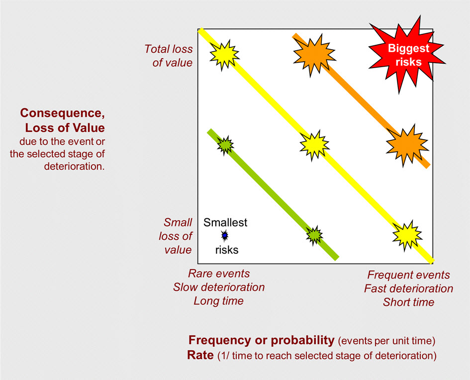
Metrics are the tool for determining whether a risk is bigger or smaller than another risk. In its list of risk metrics from various fields, the first noted by the Society for Risk Analysis (2015a) is: “The combination of probability and magnitude/severity of consequences.” Figure 1 is the map of such combinations.
For risk to heritage assets, risk is defined as “the expected fractional loss of value to the heritage asset per unit time,” e.g. % loss of value per century. In the ABC method, the risk is expressed on a 15-point logarithmic scale (analogous to the magnitude scale for earthquakes) and measurements on this scale are called the “magnitude of risk,” abbreviated MR.
Placing events and cumulative processes side by side
Although examples of risk tend to focus on rare events, risk includes frequent events and even cumulative processes. As the other risks, cumulative processes are also measured in terms of consequence, i.e. loss of value, but one must select a particular stage of deterioration or a particular time in the future to assess a combination of consequence and the time it took to get there. Thus a high rate process is comparable to a frequent event whereas a slow rate process is comparable to a rare event.
When risk is intangible
It is easy to slip into thinking that risk only measures tangible phenomena, e.g. the gradual erosion of a wall or the chance that the wall will collapse during an earthquake, but in heritage as in public health, tangible phenomena are only half of the analysis. The consequences depend on intangible phenomena, such as loss of value.
Mapping risks
The standard diagram for comparing risks
In all fields of risk assessment, the basic diagram for comparing risks uses two axes, shown in Figure 1. One axis measures how bad the event will be and is often called “Consequence” or “Impact.” In the ABC method, it is called the “Loss of Value.” The other axis measures how often the event is expected to occur and is often called the “Likelihood” or “Probability” of the event. In the ABC method, it is called “Frequency” for events and “Rate” for cumulative processes.
© Government of Canada, Canadian Conservation Institute. CCI 96638-0001
Figure 1. Map of loss of value versus frequency or rate.
Description of Figure 1.
The graph shows a three-by-three grid of star shapes representing risks. The stars increase in size from the bottom left corner to the top right corner.
Technical notes to the risk map
In semi-quantitative risk assessment, this diagram is often presented as a simple table with three rows and three columns, labelled low, medium, and high. The top right corner (High+High) and the lower left corner (Low+Low) are unambiguous as the highest and lowest risks, but determining the relative size of mixtures in between is not so obvious and becomes the goal of more precise risk analysis such as the ABC method.
The diagonal lines of different colours that connect equal size risks will only be straight if the X and Y axes are geometric or logarithmic, e.g. 1, 5, 25 or 1, 10, 100, rather than linear, e.g. 1, 2, 3. Simple risk maps in most fields do imply big multiplicative jumps between steps, not just uniform increments.
The risk management cycle
A cycle
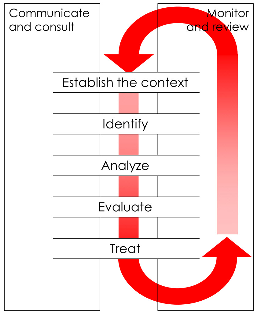
This manual is structured around a risk management cycle that was found originally in the Australian / New Zealand Standard for Risk Management (AS/NZS 4360:2004) and that is now part of the ISO 31000:2009, Standard for Risk Management. The process has five sequential steps and two ongoing activities, shown in Figure 2.
© Government of Canada, Canadian Conservation Institute. CCI 96638-0021
Figure 2. The risk management cycle.
Description of Figure 2.
A large red arrow shaped like an oval racetrack follows a path through the five steps then loops back to the top. Steps: establish the context; identify; analyze; evaluate and treat (causes). Ongoing activities: communicate and consult; monitor and review.
A starting point
All risk management methods emphasize the cyclic nature of management, but one does need to start somewhere. The first step is to establish the context — especially the scope of the initial assessment and its goals for the organization.
Assessment: The core process
The three central steps — identify, analyze, and evaluate — are the core of the process. Together, they are referred to as risk assessment.
Treat risk causes, not effects
Normally in conservation we think of the word “treat” in terms of the heritage items themselves. Here we think in terms of the risks, their causes, and their reduction.
Normal good management
We can recognize the two ongoing activities (communicate and consult, monitor and review) as standard elements of all good management, especially when acting in public trust. This manual focuses on the five sequential steps that are peculiar to risk management:
- Establish the context
- Identify
- Analyze
- Evaluate
- Treat (causes)
Analysis of a single risk
What is analysis?
Analysis is the fundamental step within any risk-based method: it is the quantification of the risk. It is the most technical part of risk-based decision making, but it is not necessarily just science. This manual emphasizes common sense, framing the questions well, and knowing where to look for technical answers.
What is analysis of a single risk?
Analysis of a single risk is an answer to a question like: What is the risk due to the “bad” boxes used to house the paper archives? Or what is the risk of theft due to the poor locks on the door? Or, what is the risk to the façade of a historic building or to the rock art in an archaeological site from outdoor weathering?
Using the manual for a single risk analysis
A single-risk analysis presumes that you already have a sense of context for the question you are asking and that you already have the risk identified, e.g. the “bad” boxes housing the paper archives will cause browning and weakening of the contents in a certain period of time.
In this case, proceed directly to step 3 of the manual, Analyze Risks. You may find, however, that you need to subdivide the risk into several parts in order to analyze it well.
Assessing risks of the same kind
What is assessment?
Risk assessment is the fundamental institutional process. It adds a step before analysis — identify the risks — and it adds a step after analysis — evaluate the risks. In terms of the five steps, assessment is steps 2 to 4:
- Identify
- Analyze
- Evaluate
What is assessment of risks of the same kind?
For example, an assessment of the risk due to lighting throughout a collection would consider many specific light-fading situations — different parts of the collection in different rooms.
As will become apparent as you do various forms of risk analyses, an assessment of the same kind of risks has the large advantage of permitting one to use the same damage criterion for all the risks.
For example, in the lighting risk assessment, this could be “a just noticeable fade anywhere on each item.” For the risk of loss of tooling detail in many stone sculptures in many locations of a site, this damage criterion could be “total loss of current remaining tool marks.” In the two examples, each risk then differs from one situation to another only in terms of the time to reach the criterion.
Using the manual for assessment of risks of the same kind
You will use the first four steps of the risk management cycle:
- Establish the context
- Identify
- Analyze
- Evaluate
Comparative risk assessment
What is it?
Comparative risk: “Comparison of two or more risks with respect to a common scale.” BusinessDictionary.com
Although the term “comparative” can be applied when the risks measured are of the same kind, e.g. comparing the weathering of one part of a site with weathering of another part of the site, we adopt the sense used in its origins — the comparison of very different kinds of risks, e.g. comparing radiation to pollution to car accidents. (Kates and Kasperson 1983) If we compare risks from earthquakes, theft, vandalism, pollution, etc., in order to decide which best to act on to preserve the asset, then we are doing comparative risk assessment.
The difficulty of comparative risk assessment
Comparing risks with different kinds of deterioration requires the adoption of a common scale to convert the predicted deterioration into predicted loss of value. This is the hard part of comparative risk assessment and the essential part. It links material science to cultural values. This conversion is described in the Analyze step.
Discovering the small magnitude of some risks
One of the primary purposes of comparative risk assessment is the recognition of greatly exaggerated risks. These are issues that “everyone knows are important” but which fail to gain significance in the cold light of comparative assessment. Some examples include the assumption that “acids” from ordinary paper boxes will somehow cause major loss to everything inside them or that the deterioration due to humidity fluctuations identical to those of the last 30 years will somehow add dramatic new damage. The exaggeration of such risks comes about from a combination of two factors: the lack of perspective in most preservation guidelines, followed by the ease and clarity with which one can identify well-known solutions — in the previous example, the purchase of acid-free boxes and the purchase of HVAC climate control. The fact that these may be extremely expensive solutions to a marginal risk or deterioration, and that perhaps the organization has bigger risks with lower cost solutions, never gets assessed.
Using the manual for comparative risk assessment
The same four steps as used in assessing risks of the same kind will be followed:
- Establish the context
- Identify
- Analyze
- Evaluate
A comparative risk assessment is not necessarily comprehensive (see next subsection). There are many reasons for limiting the identification of risks to a particular checklist, rather than a comprehensive checklist. One may be asked, for example, to assess only the risks that fall within the conservation department’s traditional responsibilities, or only the risks related to a particular design issue, such as climate control systems, or only the (many) risks due to visitors to a site.
Comprehensive risk assessment
What is it?
“(The) objective of a comprehensive risk assessment is to ensure that all pertinent knowledge, both qualitative and quantitative, is recorded, evaluated, and presented in a fashion that is understandable to decision makers." (Tardiff and Rodricks 1988)
“Comprehensive” and “pertinent” are relative — they depend on the goals of the assessment. In terms of this manual, “comprehensive” refers to the goal of minimizing all forms of loss to the entire heritage asset, whatever the causes.
Why comprehensive assessment?
To achieve the goal of minimizing all forms of loss of value to the heritage asset, we have to manage all risks and deterioration processes. We have to be comprehensive in the identification step. We have to do our best to analyze and evaluate these risks despite many uncertainties. Then we must focus on treating the largest risks.
Discovering big unknown risks
Comprehensive risk assessment will have achieved most of its value if it uncovers large risks that were not being addressed. Such risks tend to have been unaddressed because they were outside conventional areas of responsibility. Common examples include internal theft, the loss of institutional memory (staff retirement), pest risks due to careless staff behavior, etc.
How to be comprehensive
Two types of tools occur throughout risk management to aid comprehensive identification: checklists and conceptual frameworks. These are all described in the Identify step.
Using the manual for comprehensive risk assessment
The same steps will be followed as before:
- Establish the context
- Identify
- Analyze
- Evaluate
The difference is that one uses the tools of the identify step to explore as widely as possible all the risks, even those outside one’s “comfort zone.”
The communicate and consult activity becomes essential in comprehensive risk assessment because one is guaranteed to be outside one’s area of technical competence, and often outside one’s area of responsibilities. It is an institutional-wide process, and it relies on information from as many outside sources as one can obtain.
Comprehensive risk management
What is it?
Comprehensive risk management is the linkage of a comprehensive risk assessment with a risk treatment plan. It is the enactment of the full management cycle of Figure 1.
Using the manual for comprehensive risk management
The same steps as for comprehensive risk assessment will be followed, with the addition of the treat step.
- Establish the context
- Identify
- Analyze
- Evaluate
- Treat (causes)
Integrated risk management
What is integrated risk management?
There are several systems of risk management already active in organizations: disaster preparedness, public risk management, liability insurance, fire and security management, collection management, business resumption plans, etc. Integrated risk management is the effective coordination of all these systems in order to meet the institution’s goals.
Wider systems of risk management
For senior managers, risk management will already mean the framework and processes in place to deal with risks to the organization, business resumption plans, public safety, etc. Even for small organizations, risk management will already mean their approach to insurance and various forms of liability.
Heritage risk management will be integrated within the organization’s risk management systems, which encompass its legal, financial, and governance obligations. Fire management, for example, is first and foremost a life safety issue, with legal codes in place. Fire risk management for heritage assets cannot supersede life safety, e.g. single storey public buildings with easy egress may not require sprinklers to save lives, but they are a good idea to save the building.
For the very largest system, our planet, risk management has meant the implementation of sustainability as a global criterion for all contributing subsystems.
Integrating horizontally and vertically
The hierarchy of risk management systems comes about because of a hierarchy within an organization and between organizations. Each layer has its goals, responsibilities, and span of authorities. Within each layer, such as heritage management, this manual suggests that one manage all the risks that affect one’s goals (and responsibilities) in a comprehensive manner. This is one type of integration — horizontal.
On the other hand, risks due to longstanding hazards such as fire, criminals, pests, and natural disasters, or those within the jurisdiction of a particular building function, such as climate control, have well-established offices, experts, and authorities to serve them. Integration along new pathways, whether vertical or horizontal, is never easy. It will vary from informal exchange of information to formal linkages, all the way to restructuring of the organization.
Everyone is doing it
One of the advantages of adopting a risk management approach to heritage is that increasingly, all the layers above your layer (especially government) are adopting this conceptual framework. Communication will be easier and credibility more likely.
Background ideas of risk-based decision making
Rethinking disaster risk management and emergency preparedness
The old, narrow concept of heritage “risks”
In organizations, as in everyday life, we tend to think of risk in terms of fires, floods, earthquakes, war, etc. One does not plan on how to prevent such hazards, one can only plan on how to reduce losses during and after the event. This is only one type of risk — rare and catastrophic — and only one type of risk treatment — emergency preparedness.
The new, wider concept of heritage risks
Let’s take an example from the health field: the risks from cigarette smoke. We mean a range of processes, from cumulative deterioration of lung capacity that starts on the first day one inhales tars to the growing burden of carcinogens that eventually tip the body into rapid deterioration. When we think of risks to our health, we mean not only risks from smoke, but risks from earthquakes, risks from crossing the street, risks from UV, etc. In the same way that we try to balance our management of all these different risks, we must do the same for our heritage.
Integrating the rare with everything else
Emergency preparedness for heritage is usually the responsibility of the same staff that will initiate heritage risk management…you. For you, the integration is not a matter of separate responsibilities or authorities, it is a matter of linking concepts and planning that share the same goal — preservation of the heritage asset. Emergency preparedness for heritage assets will always be distinct in some of its techniques and sources of expertise — catastrophes do bring distinct problems of scale and urgency — but they are just a particular set of risks within the larger set of all risks to the asset. Doing triage or writing manuals on what to do with wet collections uses exactly the same knowledge, the same individuals, as risk management of small events.
As a planning and management element, it makes sense to integrate emergency preparedness within a system of comprehensive heritage risk management. And it may well emerge that in the light of a single measurable goal, the balance of resources currently directed to “routine” risks such as climate control, as compared to resources directed to flood mitigation, needs revision.
Integrating collections with sites and buildings
Integrating approaches
The professions specializing in heritage sites and buildings have developed their own methods and terminologies for risk management. Much of their focus has been on emergency preparedness, also called disaster planning. It is not the intent of this manual to displace those methods, nor to pretend to provide a substantive introduction to those methods.
Sites and buildings have also developed methods of estimating or ranking relative value and have encountered the same dilemmas and disputes that arise when one attempts such measures.
Although this ABC method originated with a collections perspective, we have incorporated ideas and methods borrowed from many areas of risk management, including the sites and buildings literature.
We hope that the two areas of specialization, movable and immovable heritage, both struggling to find practical and effective methodologies for wise decision making, can continue to share concepts and, perhaps, begin to build coherent integrated approaches.
The example of the historic house museum
There is one classic dilemma of heritage risk management that already integrates collections and buildings: the problem of climate control for a collection in a historic house museum. Humidification in cold climates and air conditioning in hot climates both lead to wall condensation, then mould and building decay. There can be problems of staff health, public health, and litigation.
Although not framed until recently in a risk management perspective, there is a considerable literature available on the problem and numerous museum renovations that have foundered on the dilemma.
In an innovative series of meetings sponsored by organizations for conservators of collections (American Institute for Conservation) and conservators of buildings (Association for Preservation Technology International) in the 1990s, a series of ethical guidelines were developed for decision making in such situations, called the New Orleans Charter for Joint Preservation of Historic Structures and Artifacts. (Stovel and Taylor 1996) In effect, however, these guidelines only stipulate that the decision makers consider both the collection and the building, and that they balance preservation of the two, but they do not offer a method. Risk assessment is a suitable method.
Uncertainty and anxiety
Anxiety about all the uncertainty
Everyone who applies the method experiences moments of anxiety over the uncertainty inherent in it. Uncertainty enters many parts of the risk management approach, not just uncertainty in the sense that we cannot know exactly when chance events will strike, but also uncertainty about the future context, uncertainty about the rate of cumulative processes, uncertainty about which items are affected, uncertainty about value judgements, etc.
Some anxiety is just due to the newness of the method in our field and will diminish as more of us share experiences and as experts in preservation begin to adapt to its demands.
Risk experts in other fields have developed many ways to deal with uncertainty — some of which we have adapted for this manual.
At some point, one will also wonder whether spending even longer at gathering information, or waiting for the experts to give better answers, will yield a significantly better analysis, a significantly better decision. This is the problem of “bounded rationalism,” which means simply that we make decisions as best as we can, with the best information available. We cannot wait for the perfect decision — it never comes.
The method only informs decisions, it does not automate them
In the midst of writing up difficult assessments, it will be important to remember that the purpose of this method is not to automate the decisions, but to inform the decision makers as clearly and usefully as possible. If an assessment is difficult and uncertain, then the reasons for that uncertainty become a useful part of the report. One of the decisions may well be to devote more resources towards reducing that uncertainty, so that a better decision can be made later. In any case, it is essential that risk assessment explicitly addresses the existing uncertainty and clearly communicates it to the decision makers.
Why bother?
The alternative methods — making decisions based on generalized rules, or habits, or visible improvements in facilities — while much less anxiety-provoking, provide no clear connection to the preservation goal. If the generalized rules are indeed based on sound knowledge, then that knowledge can be used much more effectively within a risk management approach. If visible improvements are known indicators of meeting the preservation goal, then that same knowledge can be put to even better use by risk management. As much as possible, the Analyze section of this manual attempts to recast established preservation knowledge within the risk management framework.
The goal of heritage risk management
The goal of conservation
Traditionally, our goal can be stated as: Preserving our heritage assets as well as possible, at the same time as providing access as well as possible, given limited resources.
Developing a measurable goal
Risk-based decision making is built on the idea that one can use some notion of value to define the goal, and that one can make some kind of rational computation to quantify all the phenomena that jeopardize that goal.
The positive perspective
Risk management can be considered a special form of cost-benefit management. From the perspective of cost-benefit analysis, and taking the example of any resource, the goal is:
- To maximize the benefits of the resource over time, as measured at some specified point in the future, and for a given cost.
A similar though not identical goal states:
- To maximize the value of the resource, as measured at some specified point in the future, and for a given cost.
The negative perspective
From the negative perspective of risk management, we can restate the goal as:
- To minimize the loss of value to the resource, as measured at some specified point in the future, and for a given cost.
The practical goal of this manual
In practical terms, and in terms of a heritage asset, we can rephrase the goal as:
- To assess the risks to the heritage, and to act to reduce them as effectively as possible, given the available resources.
Although there are subtle differences between these four stated goals, (Michalski 2008) for the purposes of the ABC method, the last two will be our guides.
Limitations of any method
“Independent of the tool, there is always a need for a managerial evaluation and review, which sees beyond the results of the analysis and adds considerations linked to the knowledge and lack of knowledge that the assessments are based on, as well as issues not captured by the analysis.”
All management tools such as the ABC method are called decision-support tools rather than decision-making tools because they assist rather than automate decisions. On the other hand, consider this statement by an author who has studied extensively which risk assessment methods have or have not worked well for public health management:
“Only a few voices want to restrict scientific input to risk management…even participants from the lay public were not only willing to accept, but furthermore demanded that the best technical estimate of the risks under discussion should be employed for the decision-making process.”
Time horizon and the social discount rate
A measurable goal requires us to specify a particular future
- To minimize the loss of value to the asset, as measured at some specified point in the future, and for a given cost.
For risks due to very rare events or very slow cumulative processes, it does not matter which point in the future we use for measuring our goal — 3 years, 10 years, 100 years — we will measure the same magnitude of risk. For risks that are frequent or fast and which reach a point of maximum damage quickly, however, it does matter — the point in time we choose for measuring the goal will change the magnitude of the risk. This means that priorities might change between different types of risk.
For example, if some pristine coloured item is subject to complete fading in 10 years by the lighting in a new exhibit, then from the perspective of the viewers of the next 10 years, this fading may be the highest risk to the asset and a priority to treat, more than the risk from theft or fire. From the perspective of viewers 30 years or 100 years in the future, however, that fading damage will have stopped long ago, whereas the chance that the item is stolen or burns increases proportionally to time. They may want us to give priority to the fire and theft issues.
Modelling the total value over time
The qualifying phrase “at some specified point in the future” in all the goals is important. Measuring the goal at different points in the future can give different priorities of risk, leading to different decisions.
In mathematical formulations of the goal, the benefits or value are accrued not at a precise point in the future, but by using a diminishing weight over time, expressed through a curve known as the social discount rate. This curve models the balance between concern for the benefits of the current generation and a slowly diminishing concern for the benefits of future generations. In this manual, social discount rate will be kept in the background, but the methods presented in the analyze step and evaluate step do take it into account, and it will be brought forward when it influences the risk-based decisions. We will, however, tend to speak of the more recognizable concept of “time horizon” or “short-term goals versus long-term goals,” rather than “the influence of variable social discount rate.”
For further discussion of social discount rate see Michalski, 2008.
The equivalence of fractional loss with the chance of total loss
Definite fractional loss versus the chance of total loss
Consider two extremes in uncertainty — the chance of total loss due to a rare event versus a completely certain loss that is only partial.
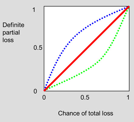
In Figure 3, one can plot the decision maker’s equivalence between definite partial loss and the chance of total loss. For example, what if one is offered a choice between a) a 50–50 chance of the heritage asset burning down in the next 75 years, and b) definite damage that will cause a loss of half the value of the heritage asset in 75 years. From the perspective of risk assessment, these two scenarios have the same magnitude of risk; they are equivalent. In Figure 3, the red line plots such equivalence. Someone who is “risk-averse” has an equivalence plot shown by the blue line: they prefer taking a definite 50% loss, rather than a 50% chance of losing everything. Someone who is risk-seeking (the green line) prefers to take a 50–50 chance of losing the whole heritage asset, rather than commit to definitely losing half of it.
© Government of Canada, Canadian Conservation Institute. CCI 96638-0023
Figure 3. Equivalence between definite partial loss and the chance of total loss. Red line: risk equivalence. Blue line: risk-averse judgements. Green line: risk-seeking judgements.
Description of Figure 3.
The X axis is chance of total loss from 0 to 1; the Y axis is definite partial loss also from 0 to 1. The line for equivalence is a diagonal straight line from the lower left corner (0,0) to the upper right corner (1,1). A blue line for risk-averse judgements starts at 0,0 and finishes at 1,1 but is curved above the diagonal, indicating that one perceives a 50-50 chance of total loss as equivalent to a 75% definite partial loss. Conversely, the green line for risk-seeking is curved below the diagonal, indicating that one perceives a 50-50 chance of total loss as equivalent to a 25% definite partial loss.
Are heritage organizations risk-blind or risk-seeking?
Part of our motivation for encouraging risk assessment in heritage organizations is our experience that they appear “blind” to risks such as fire and disasters when doing preventive conservation as compared to their full attention on slow cumulative processes, such as boxes that may be emitting acids (or not.) One might argue that this risk-blindness is a case of risk-seeking. This seems unlikely. It is more likely the general blindness problem Dörner (1996) has shown in his book The Logic of Failure, when people try to make decisions in complex systems that have either very slow feedback (in our case, very slow deterioration) or very infrequent feedback (in our case, rare disasters).
When rare events become cumulative processes
The whole notion of rare begins to diminish when one looks from the perspective of national and international agencies who advise thousands of heritage organizations. From this perspective, one sees fires, floods, major thefts, severe pest incidents, “freak” accidents, etc., on a routine basis, many events per decade, or even per year. Our obligation to provide the wisest advice to individual heritage organizations is coloured by our obligation to provide the wisest advice to all heritage organizations as a collective holding the heritage of all of us.
Summary list of tasks
1. Establish the context
- Task 1: Consult with decision makers. Define the scope, goals and criteria.
- Task 2: Collect and understand the relevant information.
- Task 3: Build the value pie.
2. Identify risks
- Task 1: Assemble the appropriate tools and strategies.
- Task 2: Survey the heritage asset and make a photographic record.
- Task 3: Identify specific risks, name them, and write their summary sentences.
3. Analyze risks
- Task 1: Quantify each specific risk.
- Task 2: Split or combine specific risks, as needed.
- Task 3: Review and refine the analyses.
4. Evaluate risks
- Task 1: Compare risks to each other, to criteria, to expectations.
- Task 2: Evaluate the sensitivity of prioritization to changes in the value pie.
- Task 3: Evaluate uncertainty, constraints, opportunities.
The risk assessment is now completed. The task may end here.
5. Treat risks
- Task 1: Identify risk treatment options.
- Task 2: Quantify risk reduction options.
- Task 3: Evaluate risk reduction options. An external consultant’s task may end here.
- Task 4: Plan and implement selected options.
One cycle of risk management is now completed.
Communicate and Consult
These activities are ongoing through all five consecutive steps above.
- Explain the risk-based approach if it is novel.
- Consult with experts and stakeholders, as well as colleagues.
- Make clear reports, clear graphs. Document the process thoroughly.
Monitor and Review
These activities are also ongoing through all five consecutive steps above.
- At each step, be prepared to go back and review a previous step.
- Review the risk reductions achieved by previous risk treatments.
- Coordinate future cycles within the existing cycles of the institution’s management.
Step 1: Establish the context
The three tasks for this step are:
- Consult with decision makers. Define the scope, goals and criteria.
- Collect and understand the relevant information.
- Build the value pie.
Tasks for the establish the context step
Task 1: Consult with decision makers. Define the scope, goals and criteria
Establish management support
This is an essential step in any organizational project, but especially for risk assessment because the method is unfamiliar, it asks difficult questions, and it involves many parts of the organization.
Communicate the method
Explain the risk management approach. Provide examples, resource materials, and presentations. Use graphs and tables from case studies as illustrations. Expect to do so throughout the assessment process.
Establish support for consultation with staff
Risk assessment requires access to staff knowledge. Some of this knowledge will be sensitive since it concerns security (such as discussions of anti-theft procedures) and some of it will be sensitive since it concerns failure of the organization to preserve its assets. It is essential to have clear management support for consultation within the organization. Different organizations can have very different cultures and very different agendas for the risk assessment.
Communicate before a site visit
External consultants can use correspondence prior to the actual site visit to establish many of these points. Use a written questionnaire.
Define the scope
In consultation with decision makers, establish the kind of risks that are within scope: a single risk, a fixed list of risks, or a comprehensive assessment of all risks.
Establish the target assets, which may include collections, historic buildings, and site components.
Define the goals of the project
Establish the organization’s goals for the risk assessment. Provide proposals for those unsure of what goals are possible.
Establish the time horizon
For most situations, a time horizon of 30 years is appropriate. If the scope of your task has other targets, such as a 100-year preservation mandate, or a 10-year management plan, establish which will be used to evaluate risks and to evaluate options.
Establish criteria for risk evaluation
After one has identified and analyzed risks, one will need to decide whether to do something about each one. Aside from obvious criteria such as regulations and costs, one will need guidance on what magnitude of risk is “acceptable.” It is helpful to know from the beginning of an assessment how the organization will balance use of the asset with risks due to that use.
Task 2: Collect and understand the relevant information
Key documents of the organization
These are essential to have in-hand:
- The organization's mission statement (may be called “Purpose,” “Goals,” “Mandate,” etc.)
- Statements of significance (or equivalent documentation) about the items within the scope of the assessment.
- Documentation about any value-based categorization that applies to the heritage asset being assessed.
When key documents do not exist
Build them during the risk assessment. It is common for the assessment process to uncover, and to make explicit, ideas about the heritage asset value that were previously unspecified.
Other policy documents
These are useful to have in-hand:
- Description of governance
- Policies concerning the target public
- Policies concerning use of the heritage asset
- Policies concerning preservation of the material heritage.
Operation and facility documents
These are useful to have in-hand:
- Organizational chart
- Financial documents
- Building plans
- Disaster plans
- Loan forms
- Incident registers
- Climate control records
- External suppliers of services and products that impinge on the material heritage
- Results of previous consultations.
External documents
These are useful to know about:
- National and international laws and other legal instruments regulating the use, protection, ownership, and control of cultural heritage
- Government policies and orientations concerning cultural heritage and risk management.
Communicate before a site visit
The questionnaire sent prior to the site visit should contain a request for all key documents listed above.
Task 3: Build the value pie
Communicate and consult extensively
Building the value pie requires extensive communication of the idea and goals behind it and extensive consultation to quantify the relative value of the groups and subgroups of items within the heritage asset.
Establish the boundaries of the heritage asset being assessed
Clarify which part of the heritage asset of the organization is within the scope of the risk management plan or of this particular assessment.
Identify the main "groups" within the asset
Make a list of the main categories or groups of items that constitute the heritage asset, e.g. Site, Building, and Collection. Groups often reflect organizational structure. For a small assessment, there may be only one group, e.g. Collections or Site.
Identify the “value subgroups” within each group
Divide each group of items into subgroups of similar value for the organization and its mandate, e.g. building elements A, building elements B, etc. If the organization already has established categories of value which apply to the heritage asset, use these as value subgroups, e.g. treasures, above average items, and average value items.
Make a draft of the value pie table
Make a first draft of the table containing the identified groups and their value subgroups. Account for all items in the heritage asset.
Define items and count them
Define clearly the individual items in each value subgroup, in whatever form makes sense for communication and for analysis. Count the number of items in each value subgroup.
Determine the relative values
Quantify the relative value of groups and value subgroups. The goal is to derive the fractional value of each item relative to the whole asset, e.g. each average painting holds 0.1% of the asset value.
Generate the value pie graphics
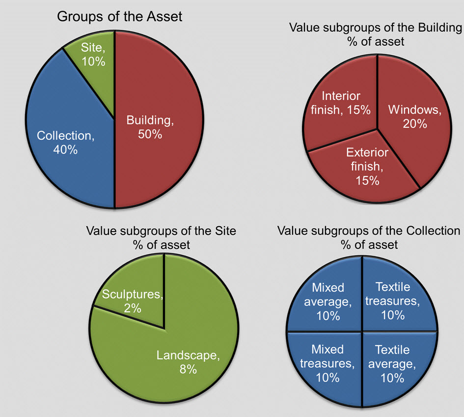
Create pie charts from the value pie tables (as shown in Figures 4 and 5). Discuss with stakeholders whether the relative size of segments in the value pies appear correct, and adjust the tables if necessary.
Besides the CCI Risk Management Database, spreadsheet software such as Microsoft Excel® or OpenOffice Calc can be used to automate calculations and to generate the corresponding pie chart(s).
Document the process
Document the entire process of building the value pie, in particular all justifications and arguments used to establish the relative values of the groups and subgroups.
Explanations for the establish the context step
Task scope and time horizon
Identify the purpose of your task
Your task might be a single risk analysis to support a specific conservation decision, or it might be comprehensive risk management to develop and implement cost-effective measures to treat the largest risks to your heritage asset over a number of years.
What is the scope?
Scope refers to the boundaries within which you will analyze, assess, or manage risks. The widest scope includes all possible risks to all items of the heritage asset, irrespective of their location or situation — on site, on exhibition, on-site and off-site storage, on loans, during transport, cataloged or not, etc. It will probably require the expertise of many professionals and the responsibilities and authorities of all layers of the organization. In many cases, however, the scope will be limited to a certain set of risks and/or to a specific portion of the heritage asset, e.g. the management of theft and mechanical damage risks during a travelling exhibition of ceramic items, or the risks to an archaeological site from flooding during the next year.
Tasks with narrower scope will likely be less demanding in terms of expertise, degree of organizational involvement, time, and resources. In any case, it is necessary to discuss and define the roles and responsibilities of the different people and parts of your organization participating in the task and to agree upon what will be its deliverables or products.
Which time horizon do you consider?
Consider the time horizon in relation to the risks which will be analyzed, assessed, and managed. Using different time horizons (for instance, 3, 10, 100, or 300 years into the future) will change the magnitudes of some risks and possibly the priorities in treating them. Selecting a given time horizon means that you have decided to measure risks from the perspective of that moment in time when the asset is “handed over” to future owners.
Mandate, policies, and procedures of the organization
What is the organization’s mandate?
The organization’s mandate (or mission statement) contains the official instructions about the purpose and core responsibilities of the organization, including clear statements about what to preserve and how to use the heritage asset. It serves as a reference within the organization to judge the significance of these items — individually, in relation to each other, and in relation to items not belonging to the heritage asset. It also guides decisions about acquisitions, access, insurance, etc.
Find the policies and procedures that can guide and support your task
Policies are written statements that communicate management’s intent, objectives, requirements, responsibilities, and/or standards concerning the activities of the organization. Procedures describe how each policy will be put into action within the organization. The presence or not of effective policies and procedures will influence many risks to your heritage asset, through activities such as collection management (acquisition, documentation, conservation, lending, deaccessioning), building and site management, user access, public safety and security, disaster preparedness, and insurance.
Coordinate with existing risk systems
There are usually established systems inside and outside the organization that “manage” particular risks to the heritage asset. Each tradition of “risk management” or “security” will speak a different technical dialect and may be wary of collaboration, but they can be an essential source of information for risk assessment, as well as part of an integrated risk management plan.
Legal context
How does the legal context affect risks?
The legal context includes the laws by which your organization and its operation are bound — national and international laws and other legal instruments regulating the use, protection, ownership, and control of cultural heritage. Pay extra attention if the scope of your task includes legally sensitive issues like access to information held by public bodies, first nation or indigenous heritage, illicit traffic, international loans or trade, human rights, and intellectual property.
An international database
An online UNESCO Database of National Cultural Heritage Laws offers access to both national and international legislation related to cultural heritage.
Financial context
Questions
- Is there a conservation/preservation budget in your organization?
- How big and flexible is it?
- How and by whom is it implemented and managed?
- What is the financial value of your heritage asset?
- How is the financial situation in the heritage sector in your country?
- What financial changes, challenges, and opportunities do you expect for the future?
Understand your planning cycle
Understanding how your organization plans and operates financially will put you in a better position to assess risks, to develop risk treatments, and to obtain the funds necessary to implement them.
Especially for implementation of ongoing or long-duration tasks, it is important to incorporate their budgetary requirements into the overall, long-term financial plan of the organization. If necessary and possible, look for extra-budgetary funding opportunities within the financial context of your task.
Governance context
What is the governance context?
Finally, it is important to know how your risk-based task relates to and fits into the policies and orientation of your government towards culture and heritage, as well as into the policies concerning the use of risk management as a tool to improve the performance of government organizations. This is particularly relevant if your organization is a government agency or part of one. Understanding this context and adapting to it provides an effective way to obtain governmental support and to find synergies and develop collaboration with governmental agencies for the implementation of your task.
Contexts change over time
As with all elements of context, the legal, financial, and governmental frameworks are dynamic and will change with time. Keep in mind that it is necessary to keep monitoring and reviewing the context of your risk-based task in order to make the necessary adjustments to allow its successful implementation.
Stakeholders
Who are they?
Any person or organization who can be impacted by or cause an impact (positive or negative) on the activities of your organization and, in particular, on your risk-based task should be considered. These persons and organizations are referred to as stakeholders. They can be both internal and external to your organization. Internal stakeholders include, for instance, the directors, employees, and managers in different layers and departments of the organization, the board of trustees, and shareholders. The organizational chart is a useful tool to help identify internal stakeholders and their hierarchical structure within the organization. External stakeholders include the public and (local) communities related to the heritage asset, tourists, scholars, donors and sponsors, external suppliers of services and products, government agencies, etc.
How do they affect your task?
The impact of stakeholders on your risk-based task will depend on their level of power, influence, interest, and support concerning the task. As you proceed with the identification of stakeholders, it is useful to assign priorities to them according to their importance to the task ahead. Several techniques of Stakeholder Analysis and Mapping are available to help do that, e.g. the article in Wikipedia on Stakeholder analysis.
Engage them
Stakeholders in your heritage asset might perceive risks and their magnitudes differently because of different needs, interests, value systems, assumptions, concepts, etc. Since they can have a significant impact on the risk-based decisions to be made, it is important to develop cooperation between the main stakeholders and the risk assessment team. This includes understanding, discussing, and incorporating their input into the process; involving and engaging them to support risk management strategies by indicating their benefits, costs, etc. Failure to identify and involve major stakeholders from the beginning and throughout your risk-based task will jeopardize its successful implementation.
The value pie: Introduction
Why a value pie?
Most of us, and most organizations, have always applied more care to “more valuable” things. The value pie is just a pie chart that shows us how value is distributed throughout the heritage asset.
Risk management must take into account differences in relative value if one is to allocate resources wisely.
What values?
For purposes of this method, “value” is a single parameter that equates to relative significance, or relative importance, of the item. It takes into account and encompasses all component values identified as relevant by the organization and other stakeholders, such as aesthetic, historical, spiritual, etc. The primary guidance to quantify the relative value of items for risk management purposes will be the organization's mandate and the judgements of stakeholders.
Isn’t quantification of heritage value meaningless?
The value pie is not a measure of absolute value. It is not about precise numbers. It is about quantifying, as best we can, the shared feeling that some things are more important than others, so that the priorities established by the risk assessment reflect this feeling. Often, it is simply about specifying what things are similar in value: is a box with 1000 photographs in an archive of 100,000 photographs similar in value to one painting in the collection of 100 paintings?
Don’t values change over time?
Yes. The value pie is not a permanent judgement. It only serves the purposes of this particular risk management cycle. It can and should be modified to reflect changes in value assessments over time.
Use tools to automate calculation
The manual provides examples of the value pie tables, and later their use during analysis, so that a reader can understand the calculation and even perform the calculations manually if necessary, but it is recommended that one use spreadsheet software such as MS Excel® or OpenOffice Calc or the CCI Risk Management Database to make the tables and the value pie graphic.
Use the value pie for visual guidance
The value pie has been developed through experimentation with various groups of students and users. All pie charts take advantage of our ability to understand and judge the relative size of pieces in relation to each other and to the whole. For most people, such diagrams are much more meaningful than numbers. Automated spreadsheets or databases plus a projector allow stakeholders to explore various settings of the pie chart numbers, to see which one “looks about right.”
The value pie: Setting up the table
The asset
The “asset” refers to the whole heritage asset. The example provided is for an asset that has a site, a building, and various collections of artifacts.
Groups
Groups are the first level of division of the asset. In the example of Table 1 and Figure 4, there are three groups: Building, Collections, Site. These have been assigned 50%, 40%, and 10% respectively.
Value subgroups and item count
Value subgroups contain items of equal, or nearly equal, value. In the example of Table 1 and Figure 4, the Collections group has been divided into 4 value subgroups: “Textile treasures” containing 6 items; “Mixed treasures” with 4 items; "Textiles, average" with 1200 items; and "Mixed, average" with 10,000 items. These have been assigned equal slices of the value pie of the Collections group, 1/4 or 25% each. Note that the number of items in each value subgroup is not the same.
The Building group has been divided into 3 value subgroups: 12 windows of equal value (representing together 40% of the value of this group), 1 exterior finish (30%), and 1 interior finish (30%).
The two value subgroups identified within the Site group are: 14 sculptures of equal value (representing together 20% of the value of the site group), and 1 landscape (80% of the site group).
During risk analysis, if necessary, it will be possible to consider different fractions of the interior or exterior finish of the building when analysing different specific risks (similarly for landscape in the Site group.)
Item as a % of the asset
The final column of the Value Pie Table is a key parameter for risk analysis and must always be checked for consistency in order to validate and, if necessary, adjust the % values assigned to the different groups and subgroups. It is the value of each item expressed as a fraction (%) of the whole asset.
In the example, the collections have many more items, but since the Collections group has been assigned equal value to the Building group, each “mixed average” item in the Collections group carries only a very small fraction of the entire asset value, about 0.008%.
On the other hand, each window of the building represents about 1.7% of the value of the whole asset; in other words, each window is valued as equivalent to ~200 of the “mixed average” items in Collections. It can be confusing at first to see such large ratios between items, but they arise simply because groups with very different numbers of items have been given similar total value.
If these results don’t “feel right,” then experiment with the fractions assigned to groups and subgroups. Look for consistency with the organization’s mandate and the judgement of stakeholders. In this example, the ratio is correct because these few windows are essential to the building, and the building is more important than the collection.
| Group | Group as % of the asset | Subgroup | Number of items in the value subgroup | Value subgroup as % of its group | Value subgroup as % of the asset | Each item as % of the asset |
|---|---|---|---|---|---|---|
Building |
50% |
Windows |
12 |
40% |
20% |
1.7% |
Building |
50% |
Exterior finish |
1 |
30% |
15% |
15% |
Building |
50% |
Interior finish |
1 |
30% |
15% |
15% |
Collections |
40% |
Textile treasures |
6 |
25% |
10% |
1.7% |
Collections |
40% |
Textiles, average |
1200 |
25% |
10% |
0.008% |
Collections |
40% |
Mixed treasures |
4 |
25% |
10% |
2.5% |
Collections |
40% |
Mixed, average |
10,000 |
25% |
10% |
0.001% |
Site |
10% |
Landscape |
1 |
80% |
8% |
8% |
Site |
10% |
Sculptures |
14 |
20% |
2% |
0.14% |
© Government of Canada, Canadian Conservation Institute. CCI 96638-0025
Figure 4. Value pies for an asset with three groups and several value subgroups (derived from Table 1).
Description of Figure 4.
There are four pie charts, one large and three small. The large pie chart shows three pieces representing the building at 50% of asset value, the collection at 40% of asset value, and the site at 10% of asset value. The three smaller pie charts show the value subgroups within each of these three pieces, with the same percentages as defined in Table 1 under value subgroups.
The value pie: Using value categories
When value categories exist already
Your organization, or your nation, may already have a system for classifying cultural heritage items into different levels of value, according to predefined criteria. For example, the U.S. Library of Congress has established five levels of value for its collections, named after precious metals:
- Platinum: irreplaceable of the highest intrinsic value
- Gold: significant cultural, historical or artifactual importance
- Silver: materials at increased risk of theft or damage due to fragility
- Bronze: little or no significant cultural, historical or artifactual importance, generally replaceable
- Copper: materials held temporarily
(Hamburg 2000, p. 68)
If this is your situation, use the existing classifications to construct your value pie. In our experience, however, such classification systems are not often in place, and the assessor becomes the first to propose one.
When curatorial categories may apply
If no system exists, then it might be useful to look at the curatorial organisation of the heritage asset. It is possible that the value groups coincide with or are derived from already existing groups of items in the heritage asset, e.g. by typology, by sub-collections. In the example of the previous box, both value categories (“treasures,” “average”), and curatorial categories (“textiles,” “mixed collections”) are used in combination. Such mixtures are common and relatively convenient to use.
When categories need a process of consultation
If there is no value-based categorization that applies to your heritage asset, the best way to determine the number and the relative importance of value subgroups, i.e. the number of slices and their size in your value pie, is through a participatory consultation process involving the organization’s staff, external experts, and other stakeholders. The consultation should be guided by your organization’s mandate and policies, alongside statements of significance.
Discuss within the group if all items of the heritage asset have equal value, which typically is not the case, or if there are items or groups of items with different values, e.g. national treasures, special items, general items. How many different levels or groups of item value can you identify in the heritage asset? How do they compare with each other in terms of their contribution to the value of the whole asset? Discuss, build consensus, articulate your answers in a transparent way, and document them. Sometimes it helps to consider hypothetical situations such as: if there was a fire, which item(s) or group(s) of items should be saved first and why?
Keep it simple
Keep your value pie as simple as possible, with the smallest necessary number of meaningful value categories.
The value pie: When items aren’t so easily defined
Examples of easy to define items
Art items: e.g. paintings, polychromes
Precious items: high value confers identity
Decorative arts: practical functionality confers clear-cut identity, e.g. tools, cabinets, utensils
Distinct elements of any complex heritage asset: windows, doors, etc. of a building, sections of a dig
Examples of ambiguous items
Cabinets, shelves or boxes of related things: e.g. archival fonds, natural history specimen sets, related archaeological fragments
Cabinets or boxes of many small things: e.g. badges, bones, shards, boxes that have never been catalogued
Assets measured by their footprint: e.g. kilometers of archive shelving, square meters of archaeological site
Back to the goal for guidance
Heritage risk management has the goal of minimizing loss of value to the heritage asset, so we can allow flexibility in item definitions as long as it makes the achievement of that goal as simple and reliable as possible.
Simple and reliable for asset value
The definition of “an item” that you choose for assessment purposes must be able to capture the treasures amongst the common items. In the case of “equal value items,” the items must truly represent equal value items (more or less!). For example, if you decide to count each photographic negative as an item, is it equal in value to a whole movie reel or a print? Whatever one feels is the main value of the asset, it must be possible to apportion it meaningfully to the items selected.
Simple but reliable for analysis
In mixed collections of many boxes of small items, one will always be balancing feasibility of the risk analysis with reliability: do you count boxes whose contents will yield a highly uncertain risk analysis, or do you analyze each item in a project that will take hundreds of person-years?
Some collections, especially archives, natural history collections, and archaeological collections, have very large numbers of small items of similar value, systematically organized in boxes on each square metre of floor or each metre of shelf and can be counted by these units of volume. Fortunately for risk assessors, such collections usually know very well which ones are their precious items.
Simple but reliable for treatment
Designing risk treatments such as improvements in facilities or fixtures is much simpler if items have already been quantified in practical units such as metres of shelf, numbers of boxes, etc.
The value pie: Using values directly as intangible items
A reminder of the meaning of “item”
In this manual, “items” are simply the smallest meaningful constituents of the heritage asset, where “meaningful” is in terms of risk management. They do not have to be single objects; they do not even have to be tangible, but they do need to help the quantification of risk and risk treatment.
When items can best be tangible things
For museums, libraries and archives, items are usually obvious — the objects themselves — although as noted in other sections, an item may become a metre of shelving or a fonds.
For buildings and sites, items can also be physical components. A group may be a building, and its items may be its components, such as windows, walls, special decorative elements, etc. This is especially true whenever the local manager is already in the habit of pointing out components that carry most of the recognized value, such as a rare type of original window or an elaborate decorative detail.
If, in addition, such components have particular vulnerabilities to particular hazards (wooden windows to rot, plaster decorations to abrasion and vandalism) then risk analysis will be easier, more meaningful, and more precise if one uses these physical components as items for the value pie. Risk treatments will also be better identified and evaluated.
When items can best be intangible things: Values and attributes
Many of the formal guidelines for building and site management are formulated now in terms of values or attributes. If it is more meaningful for the managers and stakeholders, more easily linked to other assessments, more easily and reliably analyzed in terms of specific risks, then one should use values or attributes as the items in the value pie.
How to set it up
Consider the use of the four values proposed by English Heritage: Evidential, Historical, Aesthetic, Communal. (Drury and McPherson 2008) Table 2 shows the value pie for two buildings. Note that there is only 1 “item” in each value subgroup. In this example, the 4 “items” are assigned as equal in Building B but different in Building A.
| Group | Group as % of asset | Value subgroup | Number of items in value subgroup | Subgroup as % of group | Subgroup as % of asset | Item as % of asset |
|---|---|---|---|---|---|---|
Building A |
80% |
Evidential value |
1 |
20% |
16% |
16% |
Building A |
80% |
Historical value |
1 |
20% |
16% |
16% |
Building A |
80% |
Aesthetic value |
1 |
20% |
16% |
16% |
Building A |
80% |
Communal value |
1 |
40% |
32% |
32% |
Building B |
20% |
Evidential value |
1 |
25% |
5% |
5% |
Building B |
20% |
Historical value |
1 |
25% |
5% |
5% |
Building B |
20% |
Aesthetic value |
1 |
25% |
5% |
5% |
Building B |
20% |
Communal value |
1 |
25% |
5% |
5% |
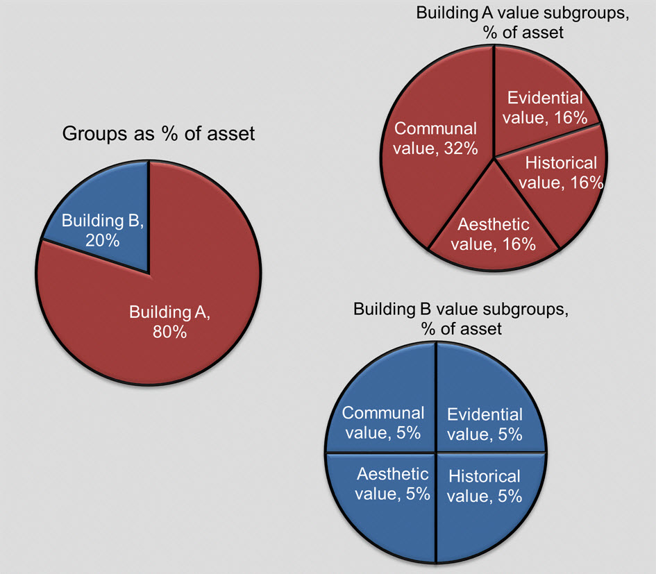
© Government of Canada, Canadian Conservation Institute. CCI 96638-0027
Figure 5. Value pies for two buildings using values directly as intangible items (from Table 2).
Description of Figure 5.
The largest of the three pie charts shows two pieces representing the groups of Table 2. These are Building A at 80% of the asset value and Building B at 20% of the asset value. Two smaller pie charts show the subgroups within these buildings, with the same percentages as defined in Table 2.
The value pie: Multiple contributing values to each item
Weighted contributing values
This example follows the general pattern of weighted contributing values. Readers may be familiar with the pattern from other decision-making tools that apply weighting to multiple factors.
This is not a case of using values directly as intangible items in the value pie (discussed previously) but of the more common case of measuring the value of tangible items in terms of several contributing values, such as those listed as primary criteria in Appendix D of the Canadian government's Guide to the Management of Movable Heritage Assets.
This example considers only a single group, called “Collections.” In some situations, collections will be the entire heritage asset.
Structure the consultation process
When dealing with challenging situations involving complex heritage assets with multiple stakeholders and multiple managers in different sectors of the organization, it is important to adopt a well-structured and well-facilitated approach. The following example is a simplified version of several complex projects developed by Pedersoli.
Steps
- As a team, identify and write down clear definitions of all contributing values (e.g. historic, scientific, artistic) that determine the significance of the heritage asset (Table 3).
- As a team, discuss and quantify the relative importance of these contributing values, assigning weights to them that take into account the organization’s mandate (Table 3).
- As a team, define a suitable ratio scale to score the “degree of occurrence” of each contributing value in different items of the heritage asset. In the example given, Table 4, six steps of x3 were selected after discussion.
- As a team, identify meaningful subgroupings of items in the heritage asset. As suggested previously, one can use existing curatorial or typological categories and subcategories, i.e. are they perceived as having different relative importance? With the team, score the “degree of occurrence” of each contributing value in each subgroup of items. If necessary, divide the subgroups further if items differ significantly in relative value. If there are a few very important items within a large collection, score them individually.
- Calculate the weighted sum for each value subgroup by multiplying the scores and the corresponding weights and then adding up the obtained products (Table 5). These weighted scores indicate the relative value of each subgroup within the heritage asset.
- Calculate the relative value of each item in terms of the group and finally in terms of the whole asset.
If consensus cannot be reached about one or more specific points during the consultation process, majority vote can be used as an alternative to solve the issue, but in such cases, all arguments (pro and con) should be put forward and discussed prior to voting, documented, and permanently attached to the resulting value pie for explanation and transparency.
Items with multiple values: A worked example
| Contributing values | Definition of the value | Weight |
|---|---|---|
Historic value |
The item is directly associated with and contributes in a fundamental way to the understanding and appreciation of the country’s history over a particular period and in a given region. |
15 |
Scientific value |
The item bears information or data that (might) contribute in a significant way to scientific research and academic studies. |
5 |
Artistic value |
The item possesses artistic and/or design quality, containing items that are representative of recognized artists, styles, art, or design movements. |
1 |
| Points | Definition of the score |
|---|---|
0 |
The items do not possess this contributing value. |
1 |
The occurrence of this contributing value in the items is very small. |
3 |
The occurrence of this contributing value in the items is small (of the order of 3 times greater than that corresponding to the score “1”). |
9 |
The occurrence of this contributing value in the items is medium (of the order of 9 times greater than that corresponding to the score “1”). |
27 |
The occurrence of this contributing value in the items is large (of the order of 27 times greater than that corresponding to the score “1”). |
81 |
The occurrence of this contributing value in the items is very large (of the order of 81 times greater than that corresponding to the score “1”). |
243 |
The occurrence of this contributing value in the items is exceptional (of the order of 243 times greater than that corresponding to the score “1”). This score indicates the maximum intensity of the occurrence of this feature throughout all components of the heritage asset. |
| Value subgroup | Historical value points | Scientific value points | Artistic value points | All points | Subgroup as % of the group |
|---|---|---|---|---|---|
Value subgroup A |
243 x 15 |
243 x 5 |
3 x 1 |
4863 |
4863/10504 = 46.3% |
Value subgroup B |
243 x 15 |
81 x 5 |
27 x 1 |
4077 |
4077/10504 = 38.9% |
Value subgroup C |
9 x 15 |
3 x 5 |
1 x 1 |
151 |
151/10504 = 1.4% |
Value subgroup D |
81 x 15 |
9 x 5 |
3 x 1 |
1263 |
1263/10504 = 12.0% |
Value subgroup E |
9 x 15 |
3 x 5 |
0 x 1 |
150 |
150/10504 = 1.4% |
Totals |
- | - | - | 10,504 |
100% |
| Value subgroup | Subgroup as % of the group | Number of items in the subgroup | Item as % of the group Collections (and of the asset since only one group) |
|---|---|---|---|
Value subgroup A |
46.3% |
2220 |
46.3%/2220 = 0.021% |
Value subgroup B |
38.9% |
9800 |
38.9%/9800 = 0.0040% |
Value subgroup D |
12.0% |
148 |
12.0%/148 = 0.081% |
Value subgroup C |
1.4% |
120 |
1.4%/120 = 0.012% |
Value subgroup E |
1.4% |
5620 |
1.4%/5620 = 0.00025% |
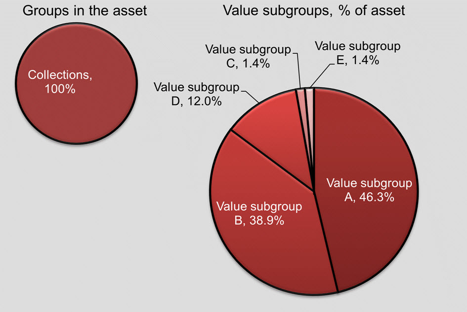
© Government of Canada, Canadian Conservation Institute. CCI 96638-0029
Figure 6. Value pies from Table 6.
Description of Figure 6.
There are two pie charts, one large and one small. The small pie chart shows that the asset has only one group, called Collections. The large pie chart shows the value subgroups A, B, C, D, and E listed in Table 6. They are sorted from largest to smallest: A, B, D, C, E.
The value pie: Capturing ensemble value
What is an ensemble?
An ensemble is a group of heritage items that acquires significant value due to the existence of the group. In poetic terms, the whole is greater than the sum of its parts. Although one can argue that all heritage collections are ensembles, we are concerned here with situations where consideration of ensembles radically changes the risk analysis. The three types of ensemble, in increasing complexity, are:
- a set of identical items which must be complete, e.g. dishes, playing cards, temple columns;
- an assemblage of dissimilar items that make up a functional entity, e.g. the doors, windows, walls, etc. that make a building; and
- a group of items with a shared association, e.g. the original items in the room of a famous individual.
What is ensemble value?
For purposes of risk analysis, ensemble value is the value inherent in the ensemble per se that is lost when any one of the items in the ensemble is lost. Ensemble value is lost with the first loss of an item from the group; it cannot be lost again when a second and a third item is lost.
Two methods for ensemble analysis
There are two methods for analyzing ensembles:
- the ensemble is one big item
- the ensemble is the individual items plus an added ensemble item (which is intangible).
The choice will affect both the way one constructs the value pie and the way one does the risk analysis.
The “one big item” method
This is the simplest method. One considers the ensemble as one item, e.g. one set of dishes, one building, one room of original furnishings as used by the famous personage. This method applies best when one (or more) of the following applies:
- When the heritage value resides primarily in the ensemble, i.e. the group only has value as a complete set.
- When one cannot meaningfully analyze loss of value other than considering the ensemble as a single item.
- When one has many ensembles to consider. This implies that ensembles are the relevant item for the organization.
The “added ensemble item” method
This method allows one to consider both the value of each item on its own and the ensemble value. One enters the individual items, but one also adds a new item that represents the intangible value of the ensemble per se. One then needs a new value subgroup to collect these ensemble items.
Test the chosen method
If one has an ensemble issue, try a quick test of the value pie method you select, and try the analysis of one risk that concerns the ensemble to see if the method works well and to see if considering ensembles is useful at all.
The value pie: Applying it to only some parts of the heritage asset
When the task concerns only some parts of the heritage asset
Depending on the objectives and scope of your task, it is possible that you decide to construct a value pie using only part of the heritage asset instead of all of it. In this case, be aware that the calculated magnitudes of risks are valid only within that part of the asset and do not apply to the entire asset!
Consider two pies if necessary
From the overall asset management point of view, it is advisable to assess risks considering the expected loss of value to the entire asset, even if the scope of your task covers only part of the asset.
In this situation, it will be instructive to construct two value pies: one for the entire asset and one for the selected part of the asset.
The value pie affects risk assessment
Ways of grouping items
One can group items in different ways when doing risk assessment. Take, for example, a museum with many black ink drawings and many watercolours on display and in storage. A few of each are very precious.
For analysis of the rate of light fading, it is best to form groups based on sensitivity to light, i.e. watercolours versus black ink drawings. For treatment, it is best to form groups based on location, i.e. storage versus display. For the value pie, it is best to form groups based on large value differences, i.e. precious versus all the rest.
For very precise disaggregation of the light-fading risk, one would use all these distinctions, but that would mean eight different specific risks (2 x 2 x 2).
If one wants to disaggregate into just two rather than eight specific risks, then it is the value pie that takes precedence. This is because loss of asset value lies at the heart of risk management and large differences in the value of items will greatly affect prioritization of risks. An optimum disaggregation might consider three risks: the precious watercolours on display, the precious watercolours in storage, and everything else.
Step 2: Identify risks
Risk identification is the process that leads to identification of specific risks that can then be analyzed.
Task 1: Assemble the appropriate tools and strategies.
Task 2: Survey the heritage asset and make a photographic record.
Task 3: Identify specific risks, name them, and write their summary sentences.
Tasks for the identify risks step
Task 1: Assemble the appropriate tools and strategies
Adjust to the scope of the task
For comprehensive assessments, systematic tools are essential, since we are trying to discover what has been forgotten and what is hidden from conventional viewpoints.
Even if the scope of the assessment is limited and clearly defined, for example, an assessment of light risk in the display areas of a museum or an assessment of risks from natural hazards to an outdoor site, you still need to identify several specific risks for analysis. If the scope is a single specific issue, such as the deterioration by light of a specific valuable item or earthquake risk to a specific structure, then one can proceed directly to the next step, analyze.
Use frameworks
The following frameworks (described later) are used to guide identification in this method:
- Agents (10 agents of deterioration)
- Types (3 types of occurrence)
- Stages (5 stages of control)
- Layers (6 layers around the heritage asset)
Use the Ten Agents and Three Types of Occurrence Table
The basic aid to risk identification when applying this method to comprehensive risk assessments is a combination of the first two frameworks above. It is called the Ten Agents and Three Types of Occurrence Table (described later). A one-page printout allows for quick note taking on-site and forces one to contemplate blank cells in the table: what kinds of risk has one forgotten? See the Explanations subsection for details.
Use other tools
The frameworks and checklists listed here are not mandatory for this method. They are tools that have proven extremely helpful over many years of teaching the method. Users more familiar with hazard categories such as earthquakes, floods, inadequate climate control, etc., can use these instead of, or in combination with, the 10 agents to categorise risks.
Use the three sources of knowledge
The three practical sources of knowledge for identification (and analysis) are:
- Regional statistics
- Local knowledge
- Scientific and technical knowledge
Documents assembled for the establish the context step generally fall into the local knowledge category.
Use correspondence prior to the site visit when appropriate
For external assessors or sometimes in larger organizations, a questionnaire could be sent prior to visiting the heritage asset to ask the responsible staff about their knowledge of prior events affecting the asset and “near misses,” as well as ask for their perception of current risks.
Task 2: Survey the heritage asset and make a photographic record
Three phases of a site survey
If time allows, there are three phases of the site survey that are best kept separate:
- The preliminary tour guided by the responsible staff
- A systematic photographic survey
- Inspection and photography of important details
Look from far as well as near
In all phases of the survey, remember to observe from far away as well as close-up. Each scale provides patterns that will help to trigger risk identification and then inform risk analysis.
Phase 1: Communicate and consult with staff
The site tour with the responsible staff helps develop essential personal rapport. It allows the assessor time to comprehend the heritage asset and the site where it is located as a concrete reality. Listen. Take notes. Use the camera rarely, if at all.
Phase 2: Make a systematic photographic survey
An efficient and systematic path for making photographic surveys is essential. A suggested pattern is described under Explanations, called “A survey path for assessment of a museum site.”
Do not presume to know what photographs you will want during risk analysis
Although one will have a preliminary understanding of the risks during the survey, it is important to understand that the photographs will serve two distinct purposes:
- Discovery by inspection and contemplation
- Illustration for communication and reporting
Use a wide-angle lens
Wide-angle photographs serve to situate a series of closer photographs. For a site, begin with wide-angle views from four points of the compass. For a building, begin with wide-angle views of the whole building from front, back, and sides. Begin a room with wide-angle views of each wall. After taking wide-angle views, begin a sequence of more detailed views.
Phase 3: Details that you know mean something
During phase 2, the systematic survey, you will see many details that mean something in terms of risk. These photographs can sometimes be made at the same time as the systematic survey, or they can be made later. Often it is quicker to do the details in a separate tour, because one uses a different setup: perhaps a different lens, different lighting, a tripod, etc.
Check photos before leaving
If you are an external assessor, you cannot revisit the site easily, and you are not an experienced photographer, check photographs at the end of the day on a computer, and redo any essential views that are missing or faulty.
File and organize the photographs soon after the survey
A survey of a small site may produce several hundred images, larger assets even more. Many different filing systems and software are available for image management. Use one that you like. Use directory trees, or tags, or both to organize the images.
Task 3: Identify specific risks, name them, and write their summary sentences
Formulate and name the risks
Using the tools, strategies, and sources of knowledge, identify and make a list of risks. Short phrases are enough. Do not worry about refining these names until later.
Use imagination and intuition
For comprehensive assessment, risk identification is as much an act of imagination and intuition as one of tools and knowledge. Do not reject any plausible risks at this stage; they can be reviewed later.
Use paper at first
Even when using tools such as spreadsheets or a database, our experience has been that the first draft of the list of risks is best prepared on a single sheet of paper or in a simple text/table document. This works best in the field and for discussion with colleagues. For beginners doing a comprehensive assessment, use a one-page printout of the Ten Agents and Three Types of Occurrence Table (Table 9).
Develop the risk summary sentences
Writing the risk summary sentence is one of the most important procedures in the method — the summary sentence is essential in framing your analysis and in communicating accurately with others.
Loss of value not essential (yet)
Although the risk method is about loss in value, it is good enough in the summary sentence to describe (future) damage. The loss of value can be added during the analysis step.
Check for “And so what?”
If you can follow the summary sentence with the question “And so what?” then it is not yet describing the risk.
Review identification
Until you complete a first draft of the analysis step and treat step, it is difficult to know whether your risks have been partitioned in the best way. Be prepared to join (“aggregate”) or to split (“disaggregate”) risks later in the procedure.
Review the risk names and summary sentences
Revise the names and summary sentences as your comprehension of each risk matures. It is not unusual to make final revisions to risk summary sentences at the end of the entire project. Often the act of communicating these issues with others will inform these revisions.
Explanations for the identify step
Identify specific risks
What is a specific risk?
By specific risk, we mean a unit or package that can be usefully analyzed and quantified. In some situations, it may be appropriate to identify a very broad possibility, e.g. the risk that any kind of criminal will steal any kind of item from among all the items currently on display. In other situations, it may be appropriate to identify a much more limited scenario, e.g. the risk that amateur thieves will steal the items that are within easy reach in the open display area. The choice depends primarily on the level of detail one can actually analyze, not on what one might wish to analyze. Before one gains experience with analysis, it is common to identify risks both too broadly and too narrowly.
Splitting and combining scenarios
It is not always obvious at the beginning of an assessment how one should “package” specific risks, so the initial list of specific risks can be expected to change as information accumulates. Do not obsess at this point about identifying each risk perfectly; there will be many opportunities during the identify and analyze steps to split or to combine specific risks.
Identification during single-risk analysis
By definition, a single-risk analysis presumes one has identified a single specific risk beforehand, but in practice this will often be illusory. A request to “analyze the risk from lighting in the museum” is, in fact, a request for a risk assessment of many specific lighting risks (various locations and various subsets of the heritage asset.) A request to “analyze the risk to the site from visitors” is, in fact, a request for a risk assessment of many kinds of specific risk, such as wear and tear, soiling, vandalism, etc.
Write the risk summary sentences
Start with a list of phrases
Start with the agents and types form, and make a list of all the specific risks, using just a simple phrase for each. These will typically be brief phrases such as: “daylight fading costumes, display” or “visitors touching the walls cause soiling,” etc.
Depending on the scope of the task, if the list begins to exceed one page, you may want to consider aggregating some items on the list. Conversely, if you have only a few diffuse items on the list, you may consider breaking them up into more precise risks.
Refine each phrase as a full sentence
The risk summary is a complete and meaningful sentence that:
- refers to the future (it is not about the past or present),
- identifies the hazard or agent (usually in the subject of the sentence),
- identifies the adverse effect (usually in the verb), and
- identifies which part of the heritage asset will be affected (usually in the item of the sentence).
Examples of risk summaries
“Daylight in the new south-facing display rooms will fade all the high-sensitivity colours in the costumes exhibited in those rooms.”
It is not always possible to keep the sentence so simple. Clarity is more important than sentence structure:
“Visitors will touch the building’s walls where they have access and deposit both oils and dirt that cause visible soiling.”
It is common for the adverse effect (“faded,” “soiled,” “stolen”) to be stated explicitly but not the consequent loss of value. This is usually not a problem, since some kind of loss of value can be presumed and will be explained later during the analysis step.
Why this emphasis on the risk summary?
It has been our experience that the ability to formulate a legitimate risk summary sentence always precedes the ability to develop a useful risk scenario and analysis. The transition between simply listing problems such as “poor humidity control” and actually formulating a risk sentence — “RH in furniture storage is likely to go below proofed RH due to recent operational changes, which is likely to cause new fractures” — marks the transition from rule-based preventive conservation to risk-based decision making.
Susceptible and exposed = affected
Susceptible parts of the heritage asset
In Figure 7, the grey rectangle represents the heritage asset. For each hazard (or agent of deterioration) there is a part of the asset that is susceptible, shown as the blue rectangle (for example, susceptible to clothes moths or susceptible to water damage). We can identify which items in our asset are susceptible to which agent of deterioration before even knowing if they are exposed. On the other hand, we must be careful not to assume that susceptible items will be affected, i.e. at risk. We need exposure to the relevant hazard to create the risk.
Exposed parts of the asset
For each hazard (or agent of deterioration), there may be parts of the asset that are exposed (shown as the red rectangle in Figure 7) and parts that are not. For example, an off-site storage room may have high exposure to insects; display areas typically have higher exposure to light; outdoor items often have high exposure to pollutants. If these areas only house items that are not susceptible to pests or light or pollutants, then there is no risk.
At risk (affected) = susceptible and exposed
Where items are both susceptible to an agent and exposed to that agent (overlapping area between the blue and red rectangles), we have that part of the asset at risk (the part that will be affected in the specific risk scenario).
Parts of the asset are not necessarily all in one place
Figure 7 is an abstraction. In reality the susceptible parts, the exposed parts, and the affected parts may be fragmented and spread all over the heritage organization facilities.
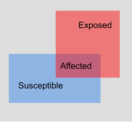
© Government of Canada, Canadian Conservation Institute. CCI 96638-0032
Figure 7. Affected items are items that are susceptible to an agent and exposed to that agent.
Description of Figure 7.
A blue square labelled “Susceptible” partially overlaps a red square labelled “Exposed.” The overlap is labelled “Affected.”
Checklists
Advantages and disadvantages
Checklists are practical and don’t require much thought but become massive in a quest for comprehensiveness. Even then, they can still fail to list a risk that a little imagination and an observant eye will deduce easily, given a method for thinking, such as frameworks.
CCI Preservation Framework Poster
A published checklist called the Framework for Preserving Heritage Collections uses two of the frameworks of this manual — agents and stages — to structure details about controlling risk. It is not a checklist of risks, but a checklist of all the details that will reduce risk. As such, it is most useful for thinking about the treat risks step. Here in the identify risks step, it serves as a list of what might be missing in your heritage organization.
Paths and schedules as organizer
The problem with many checklists, with or without a framework, is that there is little connection with the actual schedules or paths one might efficiently follow in doing the checklist. For example, on a checklist with a section on “Lighting” one may have a question about the condition of windows (outdoor survey), then a question about UV levels (indoor survey), then a question about lighting policy (documents) and then a question about exposure time (staff knowledge). In the later section on comprehensive risk identification, we suggest a sequence of activities for actually doing risk identification during a comprehensive risk assessment.
The checklist fallacy
Many checklists have been produced for preservation surveys over the last two decades, for museums, archives, libraries, buildings, and sites. Studies of the effectiveness of long checklists in airplane safety and short checklists in hospital emergency units demonstrate the following benefits:
- avoidance of oversight if a large number of things can each lead to disaster and
- consistent application of a short list of statistically proven indicators for a particular diagnosis.
Behind both these kinds of checklists, however, is a huge amount of research that established what to put in the list, whether long or short. Our field lacks such knowledge, so conservation checklists mix major issues with minor issues, without a sense of priority.
Checklists can help risk identification, but one must recognize that only analysis can decide which are important and which are not. Once our community begins to accumulate and share comprehensive risk assessments, evidence-based checklists can emerge.
Frameworks and their purpose
Frameworks used in the manual
For managing the risk management process:
- The risk management cycle (5 steps + 2 activities)
For thinking about risks in the identify, analyze, threat steps:
- Agents (10 agents of deterioration)
- Types (rare, common events, cumulative process)
- Stages (5 stages of control)
- Layers (6 layers around the asset)
Other conservation frameworks
Gael de Guichen developed a framework of “Agressors to Cultural Heritage,” organized by man-made versus natural causes with lists of risks, published as a poster by ICCROM. In the early conservation text by Plenderleith et al. (1971), there is a table called “Causes of Deterioration” that subdivides causes into chemical, biological, and mechanical categories. These frameworks, and any others available, can help prompt the identification of specific risks.
What about no framework for risk identification?
Guides to risk management for businesses and government will always provide a framework for the process itself (a variant on the risk management cycle), but many provide no further frameworks for the identification or analysis steps. They will simply suggest “scanning the environment” and “imagining what might happen.” These methods rely on the experience and expertise of the assessor.
What are the purposes of frameworks?
A framework provides a conceptual structure for thinking through a problem, a task, or a report. Its purpose is to get the job done better and to communicate the task to others better. It is not theory for its own sake. If at any point a framework begins to interfere with getting the job done well, or communicating well, feel free to adjust it, to put it to one side, or to develop your own, suited to your particular context.
Complete, but not complex
In order to do comprehensive risk assessment, one needs a framework that will push one to consider all the possible answers to the central question “What are the risks to my heritage asset?”
On the other hand, in order to remember the frameworks easily, and to communicate them clearly to others, one needs to limit the number of categories in the frameworks.
The 10 “Agents” of deterioration
A framework for the items perspective
The agents are a classification scheme for all possible hazards to the heritage asset, made from the perspective of the heritage asset itself. They allow one to think about how the hazard appears to the item. They were developed in 1981 (Michalski 1990) and used to structure the CCI poster published in 1994 as the Framework for Preserving Heritage Collections. In the 1994 edition, only the first nine agents are listed. In the second edition of 2014, all 10 agents are listed, along with issues related to sustainability.
Using the agents to identify risks
This manual uses the 10 agents of deterioration as its primary (though not mandatory) framework for organizing risks. For the identify step, imagine yourself as one of the items, and then ask: What might damage me in the future, in this location? Now use the agents one by one to focus the question: What physical forces might strike me here? Why? What thieves might steal me from here or what vandals might damage me here? Why? What fires will affect me here? Why? And so on down the list of 10 agents.
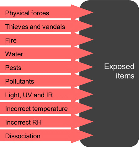
© Government of Canada, Canadian Conservation Institute. CCI 96638-0034
Figure 8. The 10 agents of deterioration that can affect exposed items.
Description of Figure 8.
The 10 agents of deterioration: physical forces; thieves and vandals; fire; water; pests; pollutants; light, ultraviolet, and infrared; incorrect temperature; incorrect relative humidity; and dissociation.
An aid, not a straitjacket
At some point, every user notes that the 10 agents are a simplification of a complex reality. From the perspective of the heritage asset, fire can split into incorrect temperature, pollutants, and incorrect humidity, and later water and dissociation. Large floods may be better classified outside the agents’ framework rather than split into water and physical forces and incorrect relative humidity (RH). It’s up to you to choose.
As with any conceptual tool, if it becomes more nuisance than aid, it can be adapted or dropped. With long experience, however, and the need for efficient strategies, one does keep coming back to these 10 agents.
See the CCI web page for details
The 10 agents of deterioration are each explained in great detail on the CCI web page.
The causal chain from hazard to adverse effect, via the 10 agents
Causality: Our overall model
The yellow, red, and white rectangles in the diagram below are some of the words and phrases that people give during a group exercise when asked simply “What are the risks to my heritage asset?” followed by “What are the causes of each risk?” and “What are the effects of each risk?” The phrases elicited can always be organized as shown, with arrows linking phrases. These cause-and-effect arrows all flow left to right, from external hazards or internal hazards via failures of resources, failures of mitigation, via the agents of deterioration, ending in an adverse effect on the asset. Each path from its beginning on the left to its end on the right constitutes a risk scenario.
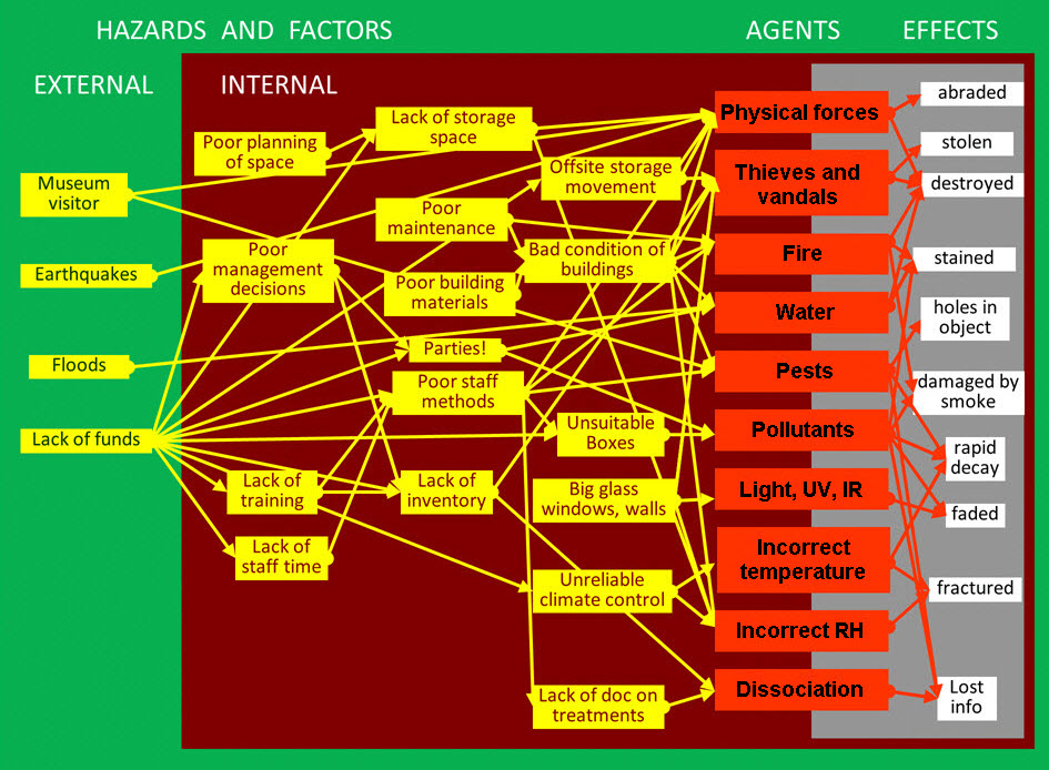
© Government of Canada, Canadian Conservation Institute. CCI 96638-0035
Figure 9. The cause and effect chains that form during the group exercise that asks simply “What are the risks to my heritage asset?” followed by “What are the causes of each risk?” and “What are the effects of each risk?” It demonstrates that the many phrases elicited by the word “risks” form links in a network of cause and effect beginning with hazards and ending with effects on the asset.
Description of Figure 9.
Examples of the path of a risk scenario. Begins with external, internal hazards combining with a failure in resources or mitigating factors. This leads to an agent of deterioration and ends with any number of resulting adverse effects on an asset. An example being the lack of funds, causes lack of training, causes poor staff methods, which leads to pests and results in holes in the object.
The agents of deterioration as a complete set of organizers
The agents of deterioration (red boxes) serve as channels to organize all the scenario paths and are located at the interface with the items themselves (the grey rectangle).
The three “Types” of risk occurrence
In terms of occurrence (timing), risks can be divided into two main groups: events and cumulative processes. For practical purposes, events can be further divided into rare and common events. The result is three practical types of risk occurrence: rare events, common events, and cumulative processes. The boundaries between the three categories are not precise; each overlaps with the next category. The purpose of the “types” framework is to guide the risk discovery process, to guide the location of information during the analyze risks step, and to guide thinking during the treat risks step.
These three types of risk occurrence do not imply anything about the size of the risk — your smallest risk and your largest risk, and everything in between, can be any one of the three types.
| Rare events | Common events | Cumulative processes |
|---|---|---|
“Rare” events occur less often than approximately once every 100 years (from the perspective of one heritage organization.) As a result, rare events are not part of the direct experience of most heritage organization staff. From the perspective of the total heritage of a nation, such events may happen every few years, and from a global perspective, these events can become routine. |
Common events occur many times per century. These are events that are part of the direct experience of many heritage organization staff or of people in the vicinity of the heritage organization. |
Cumulative processes can occur continuously or intermittently. Over the years, most heritage organization staff will have observed the cumulative effect of one or two such processes on some items, that is to say, they will have seen the item “age.” Very frequent events (more than once a year) can also be considered as cumulative processes for risk analysis. |
Examples: |
Examples: |
Examples: |
“Rare” as a rigorously defined term
Rare is relative to the time horizon
Rare can be defined precisely as events that occur less often than the selected time horizon of the risk assessment. For example, if one selects a 100-year time horizon, then rare events are those which have a mean time between events of more than 100 years. If one selects 30 years, then rare events are those that have a mean time between events of more than 30 years.
Implications for the idea (feeling) of risk
Rare events are not a “sure thing.” We think of them in terms of “chance” of happening. Common events and cumulative processes are a sure thing. Note that the distinction can only have meaning if we specify a particular time horizon and a particular heritage asset…very little that is plausible is rare if we speak of all heritage organizations and many centuries.
This distinction was noted already in the general discussion of the equivalence of definite fractional loss with the chance of total loss. Decision makers may have a “gut feeling” that a 5% chance of losing the entire heritage asset and a definite loss of 5% of the heritage asset are not equivalent, but the method assumes that they are equivalent. The method will, of course, always make clear to decision makers which risk is a chance and which is a “sure thing” from the perspective of their planning cycle, their organization. (As noted before under uncertainty, in reality even a “sure thing” is clouded by some degree of uncertainty.)
Implications for the calculation of risk
If the mean time between events is longer than the time horizon selected, then these are events that one should express as a probability, rather than a frequency or mean time between events. This makes for a subtle distinction — the probability of such events within the time horizon is not 1, i.e. it is not “guaranteed.” It is less than 1. For the standard assumption of a “normal” distribution of probabilities, for example, the probability that a 100 year event will occur in 100 years is only 0.6.
Not an issue
The necessary precision in both the conception and the calculation of rare risk is beyond the scope of the ABC method and, fortunately, not significant to the kinds of distinctions between large and small risks that we seek to uncover for heritage assets. As long as one consistently expresses all events in terms of frequency, even when it seems bizarre, then risk calculations will be correct. For example, regional data may suggest that the probability of a certain natural hazard is 1% in 100 years; this can be expressed as its equivalent frequency of “once every 10,000 years.”
The five “Stages” of control
1. Avoid
Avoid is the first logical stage and the most effective if feasible. Avoiding attractants is an important aspect of reducing pest risk, but avoiding whatever natural disasters fate has in store, other than by moving the heritage asset, is impossible.
2. Block
A barrier, somewhere between the source of the agent and the item, is probably the single most practical element of reducing risks from all agents.
3. Detect
Avoid and block will eventually fail; one needs an appropriate degree of detection for each agent or for its effects.
4. Respond
After detection, one must respond. A planned response is best, especially for large events. Some agents can only be controlled by a continuous response, as in the case of incorrect temperature controlled by mechanical systems.
5. Recover/Treat
When stages 1 to 4 fail, one can only recover, and where possible, treat damaged items. An important part of long-term recovery, however, is to learn from such failures and to improve the four previous stages. Many risk management programs begin in the light of such failures.
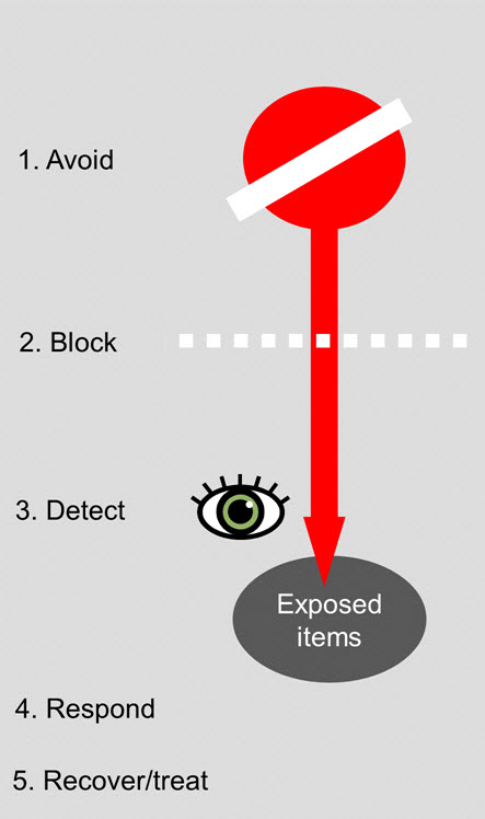
© Government of Canada, Canadian Conservation Institute. CCI 96638-0003
Figure 10. The five stages of control (Michalski, 1990).
Description of Figure 10.
A large red dot at the top of the diagram represents the source of the agent. A white diagonal bar across the dot represents the avoid stage. A large red arrow drops vertically from the source. A dotted white line cuts across it, representing the block stage. Below that, a drawing of a human eye represents the detect stage. The red arrow finally rests on a grey oval representing the exposed items.
The six “Layers” around the heritage asset
Nested enclosures
Perhaps the most ancient concept for risk management of precious artifacts was the strong box within the strong room within the strong building, situated on an easily defended site. Combined with the larger perspective of the geography within which the heritage asset is situated, we obtain the framework of “layers” shown below.
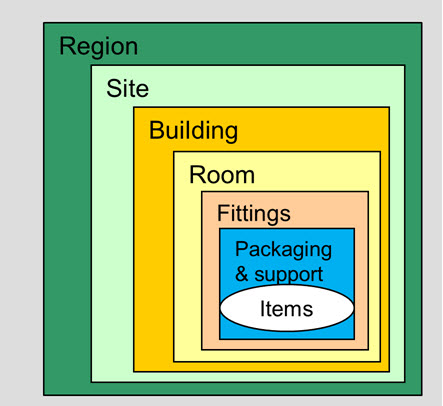
© Government of Canada, Canadian Conservation Institute. CCI 96638-0005
Figure 11. The six layers of enclosure.
Description of Figure 11.
The diagram shows the six possible layers of enclosure as six nested rectangles. At the centre is an oval labelled “Items”.
1. The region
The region is the location of hazards that we cannot avoid, but which we must understand, predict, and then mitigate appropriately.
2. The site
The site is the location of outdoor hazards, but for which we have some degree of control: drainage, lines of sight, road surfacing, barriers, etc. In many cases the site is part of the heritage asset.
3. The building
The building is the fundamental built layer around any collection. In many cases it is also part of the heritage asset.
4. The room
The room is often the location of special controls as well as new hazards.
5. The fittings
The fittings are the first movable layer, often part of a transition in responsibilities between the facilities manager and the conservator.
6. The packaging and support
The packaging and support are the closest layers to the heritage asset, always intended as protective, but they may also be a source of new hazards.
Not all heritage assets have all layers
Even when heritage assets incorporate only some of these layers, this framework can be useful to stimulate thinking about protection layers around the heritage asset.
Layers as hazards and as a structure for knowledge
Layers not only structure the analysis of the block stage of control, they also structure possible sources of hazards and agents of deterioration. For example, while each layer can block water or pollutants or fire that originates outside that layer, the layer itself can be the source of all those agents. The building can block regional rainfall but be a source of water leaks.
The layers also structure the knowledge needed for analysis: for each layer, there will be a separate body of knowledge and expertise.
The three sources of knowledge
For risk identification and analysis, there are three sources of knowledge. Conveniently, these map closely (though not perfectly) to the three types of risk occurrence, as noted in the middle row of this table 8.
| Regional statistics | Local knowledge | Scientific and technical knowledge |
|---|---|---|
These statistics are the bedrock of understanding catastrophic risks. Many agencies around the world have developed vast resources to provide non-technical users with Internet tools to predict these risks. |
This source of knowledge needs you to meet people, to discuss, to interview, and to do facility surveys, collection surveys, site surveys, etc. Do not underestimate or overestimate this source relative to the other two. This source includes the common sense and intuition of you and your colleagues. |
The CCI web page on agents of deterioration provides an introduction to the essential understanding of each agent. Beyond that, one needs to read more or talk to experts (such as those at the institutes responsible for this manual). |
This is the usual source of knowledge about the frequency and intensity of rare events. |
This is the usual source of knowledge about common events and about the intensity of cumulative hazards. The source of knowledge about all five stages of control and the local layers. |
This is the usual source of knowledge about the sensitivity of heritage assets to cumulative processes and the source for most theories that can analyze risks. |
Examples: |
Examples: |
Examples: |
Comprehensive risk identification: The Ten Agents and Three Types of Occurrence Table
{10 agents} x {3 types of occurrence}
If your task is comprehensive risk assessment, then Table 9 is a suggested list to “fill in.” It uses the 10 agents and the 3 types of occurrence. This gives 30 combinations, but in practice, a few are generally not applicable.
| Rare events | Common events | Cumulative processes | |
|---|---|---|---|
Physical forces |
- | - | - |
Thieves and vandals |
- | - | - |
Fire |
- | - | Generally not applicable |
Water |
- | - | - |
Pests |
- | - | - |
Pollutants |
- | - | - |
Light, ultraviolet and infrared |
Generally not applicable |
- | - |
Incorrect Temperature |
- | - | - |
Incorrect relative humidity |
- | - | - |
Dissociation |
- | - | - |
At least one risk per cell
The purpose of this table is not to limit the number of risks of each type — you may find many risks in a single cell. The purpose of this list is to encourage the assessor to think outside the usual habits. If one’s initial reaction is “I have no risks of this type” or “this makes no sense to me,” then imagine something unlikely or strange. You can always dismiss it later if analysis shows it to be very small.
The list can be shortened later
Some risks will be aggregated into one larger risk for assessment, either in this step or in the analyze step. Some risks will be shown by a preliminary analysis to be negligibly small. In the final report, there will always be the opportunity to note such revisions and their reasons. Be sure to make notes of all the ideas that arise during the identify step.
Comprehensive risk identification: Use efficient paths for surveys
Introduction
If you have limited access to the facilities and collections because of security or timing issues, then an efficient method for making surveys is essential. For collections and buildings, we suggest the method outlined below. In large facilities, with many windows, many doors, many rooms, many fittings, many packages, and many items, focus on documenting one representative example of each type, plus any special cases that are relevant to the risk assessment.
1. Tour the site
One circuit of the site. Note topography, drainage, lighting, neighbouring buildings, perimeter security.
2. Tour the buildings and outdoor sculptures
One circuit of each building, each outdoor sculpture:
- Look from a distance (relation of the item to the whole asset and to external hazards)
- Inspect from close-up (current state, evidence of prior damage)
For functional buildings:
- Inspect the roof (step back to see)
- Inspect the walls (from close and far)
- Inspect the doors
- Inspect the windows
3. Tour the collection rooms
One circuit of each room. Concurrently:
- Inspect the ceiling, overhead services
- Inspect the walls, external and internal
- Inspect the doors, external and internal
- Inspect the windows
- Inspect lighting, mechanical systems
4. Tour the fittings, packaging, supports, and items
One circuit of each room. Concurrently:
- Inspect the fittings
- Inspect the supports
- Inspect the packaging
- Inspect the items
5. Tour the non-collection areas
One circuit of remaining spaces.
- Document mechanical rooms, rooms with water supplies, occupants, garbage, easy access, etc.
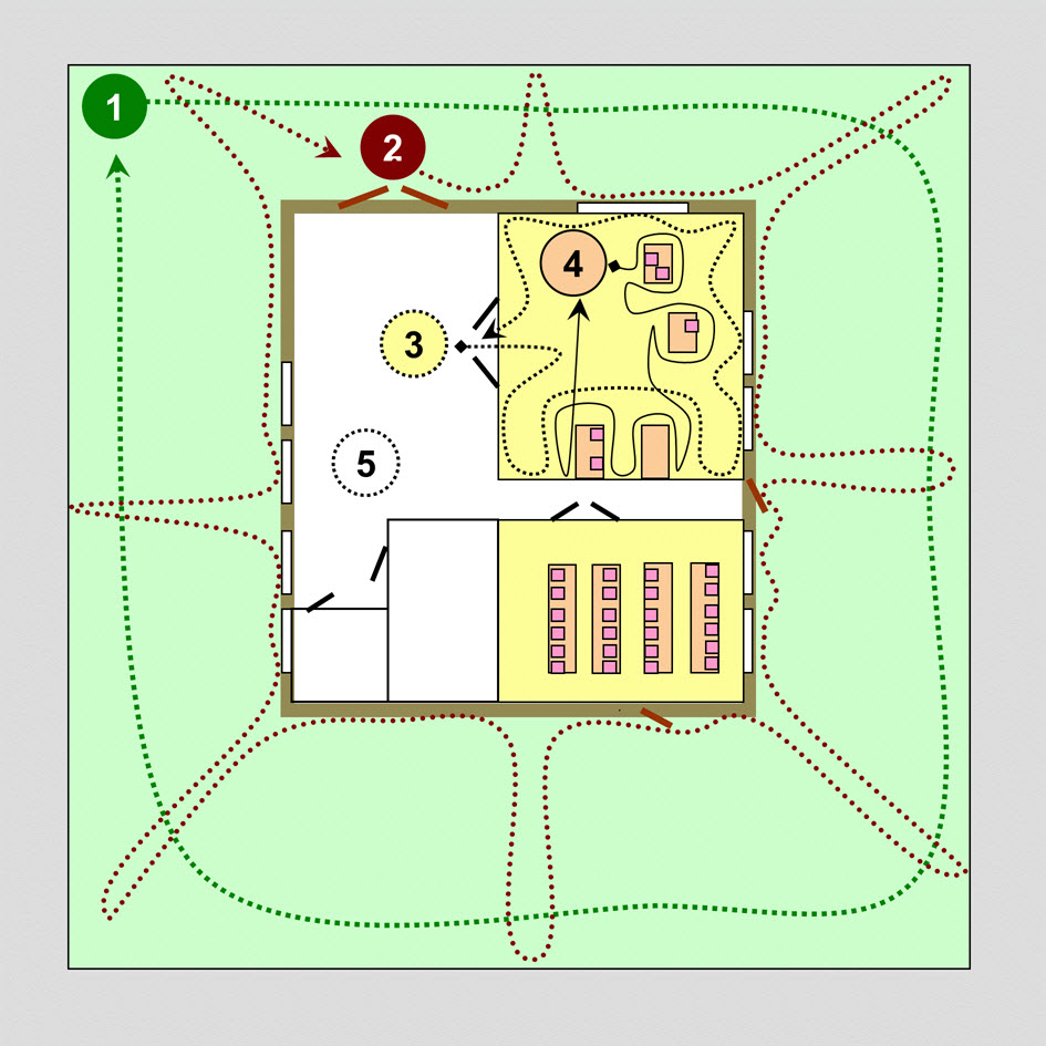
© Government of Canada, Canadian Conservation Institute. CCI 96638-0007
Figure 12. Suggested pattern for a survey of a collection within a building within a site.
Description of Figure 12.
Paths 1 to 4 of a systematic survey, as outlined in the preceding text, are shown by dotted lines. The lines emphasize the need to look from near and far when surveying the building.
Rare events and regional data
Start from common sense and local knowledge
Most of the rare events that need regional data are the “natural disasters” that we can easily imagine, such as floods, earthquakes, extreme vandalism. We can start to identify these kinds of risks simply based on what is plausible and from what we hear from staff and residents on historic events. Horror stories from heritage organizations around the world provide further inspiration — could that freak theft, breakage, arson, gas explosion, etc. happen to us too some day?? If not, why not?
Begin to collect regional data
Maps and data on the frequency and intensity of natural hazards are easy to find. These help risk identification. The careful collection of such probability and severity data, however, can wait for the analyze step (where sources of such data are described in detail).
Focus on how rare events will unfold
For rare events, the main focus during the identify step will be trying to think how such events would unfold in your organization, based on local knowledge.
Events that start small and grow
Many rare and catastrophic events are initiated by an event that is neither rare nor catastrophic, e.g. a small electrical short circuit, a visitor tripping and falling down. The question becomes: will the event escalate? Will such a short circuit cause a small fire because basic electrical safety measures were ignored by an amateur case fabricator? Will that fire spread because the cases and room are all flammable and no sprinklers are present? Is the tripping visitor likely to be in front of the most precious artifacts? Are they easily knocked down? Do they shatter easily? These details can be called “magnifying factors.”
Events that start big
Other rare and catastrophic events do have rare and catastrophic initiating events, such as major floods, earthquakes, external firestorms, etc. The question again becomes: what will happen next? Are the heritage assets above the water line? Are the item supports earthquake resistant? Can the most precious moveable items be moved quickly to safety? These details can be called “reducing factors.”
Collecting local knowledge
Collect local documents first
We suggest that a risk assessment begin with the acquisition of all relevant documents (beyond those already collected for the establish the context step), such as:
- Building plans
- Disaster plans
- Loan forms
- Incident registers
- Climate control records
Use of local documents for risk identification
Intensive study of these documents can wait until the analyze step, but a preliminary scan of these documents can provide useful suggestions for:
- Possible sources of hazards
- Contributing factors to risks
- Risk issues to raise with staff
- Places to look more carefully during the facilities, collections, and site surveys
Collect staff knowledge
Staff are an essential source of information about past incidents — fires, thefts, leaks, etc. They can provide the “inside information” on actual routines and procedures that are not formally described anywhere and not necessarily visible when you do the facilities survey.
It is important to understand the roles and responsibilities of the staff, as well as their understanding of the practical realities of the organization. Often the type of information needed for risk assessment is considered sensitive, and staff might choose not to reveal it unless they are made fully aware of the objectives, outcomes, and expected benefits of the risk assessment.
Identifying risks by causes other than the 10 agents
Ambiguities when using the agents
“Many visitors will touch the costumes within reach in the display area, causing soiling.”
The question immediately arises: does this go under thieves and vandals (a mild form of vandalism) or under pollutants (the soiling)? The short answer is that it doesn’t matter, as long as it goes somewhere. When we go to analyze and treat ambiguous risks such as this, however, we will often need the methods of analysis from both agents. We may use the methods of analyzing thieves and vandals to think about the hazard (visitor volume, ease of access) and the methods of pollutants to assess the effects (discoloration, chemical attack).
Overlapping agents
“Many visitors will touch the costumes within reach in the display area, causing soiling, or abrasions, or small tears.”
Does this go under thieves and vandals, pollutants, or physical forces? There are two options, both acceptable: place it under the agent that you expect will be the biggest consequence (effects of pollutants, effects of physical forces), or place it under the agent that is the single unifying hazard (thieves and vandals). Although visitors breaking the rules is a very mild form of “vandalism,” this agent will help us think through the analysis and treatment of the risk. The methods for estimating the frequency of touching of accessible items by visitors is exactly the same as for estimating the frequency of serious vandalism.
Complex events with multiple agents
In other words, big messy events. Disasters. Natural hazards. War.
Again, the guideline during the identify risks step is not to worry; capture the specific risk in whatever language and categories seems most appropriate. Most large events will fit under its primary agent — physical forces, fire or water.
Later, during the analyze, evaluate, and treat steps, it will become clear whether it helps, or not, to disaggregate large complex risks.
Step 3: Analyze risks
Risk analysis is the process that leads to a measurement of each specific risk identified.
Task 1: Quantify each specific risk.
Task 2: Split or combine specific risks, as needed.
Task 3: Review and refine the analyses.
Tasks for the analyze step
Task 1: Quantify each specific risk
Develop the risk scenario (optional)
In teaching beginners, we emphasize the writing of a one-page “risk scenario” prior to quantification of the three components A, B, and C. This is an expansion of the summary sentence into a complete but succinct story, with all key data. With experience, however, a good risk summary sentence is enough before proceeding to quantification of the three components of risk:
- A. Frequency or rate
- B. Loss of value to each affected item
- C. Items affected (expressed in terms of the value pie)
During the analysis of each component, keep notes of the exact argument and data you are using to justify your score.
Analyze A: Frequency or rate
For individual events:
- Determine the frequency, i.e. mean time between events.
For an accumulation of damage, decide which of these two approaches works best:
- Select a particular stage of deterioration and analyze how long it takes to reach this stage
- Select a particular time in the future, such as 10 years, 30 years, or 100 years, and move on to analyzing B.
Assign an A score to the risk.
Analyze B: Loss of value to each affected item
First analyze the physical damage that results from the individual event, or the accumulation of the process, or the multiple common events.
Now analyze the loss of value to each affected item that results from this damage.
Assign a B score to the risk.
Analyze C: Items affected in terms of the value pie
The value pie provides the fractional value of each item relative to the whole asset, so that any group of affected items can be assigned the correct fraction of the whole asset value.
Assign a C score to the risk.
Analyze A, B, C in the order that helps most
Sometimes analysis proceeds more logically in a different order than A, B, C. For example, it is often best to first analyze the items affected (C) before attempting to analyze the loss to each item (B).
Calculate MR = A + B + C
Determine the A, B, and C scores using the five point A, B, and C scales. Add the three scores to obtain the Magnitude of Risk (MR).
Provide high and low estimates
For each of A, B, and C, make a high estimate and a low estimate to reflect the uncertainty in the central estimate. This provides three estimates of MR: probable, high, and low.
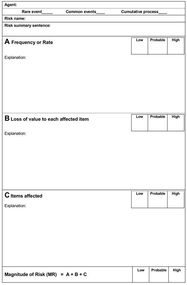
© Government of Canada, Canadian Conservation Institute. CCI 96638-0008
Figure 13. An example of a form for the analysis of each specific risk. Scores are entered in the small boxes on the right. Explanations and notes often extend to other pages.
Description of Figure 13.
The form requires the agent of deterioration, the risk name, the risk summary sentence, and each of the A, B, and C scores, with an explanation of each. The bottom of the form has boxes for the magnitude of risk score.
Task 2: Split or combine specific risks, as needed
Be prepared to split or combine risks
During analysis, and also during later steps of evaluate and treat, you may discover that it makes sense to revise the division of risks. This is normal; even highly experienced assessors are unlikely to “get it right” in the identify step.
Split when high estimates prompt new scenarios
Consider for example: “Thieves will steal artifacts.” As one begins to think about all kinds of theft scenarios, and the data that supports them, one will find that the high estimate of frequency comes from considering easily reached objects on open display. On the other hand, the high estimate of the value of the artifacts affected will be based on more difficult to reach objects, perhaps in cases or even in special storage. It is much more accurate, and more useful when developing treatment options, to split such risks. In this example, one could have “Thieves will steal high value artifacts from storage during closed hours” as a separate risk from “Opportunistic thieves will steal small, easily accessible objects from open displays during open hours.”
Split to reduce uncertainty
It can often be more precise to analyze several distinct risks rather than one ambiguous one. It can also often be easier and quicker.
Split when the scope requires it
Decision makers may be looking for a detailed assessment in order to see detailed patterns of risk across a site. This should be clarified during the establish the context step.
Combine for simplicity
It may become obvious during analysis that several specific risks can be added together without increasing the uncertainty.
Combine if knowledge is limited
Many risks simply do not have enough facts or theories to allow multiple detailed scenarios, even if we can imagine them clearly.
Keep the old specific risks for later
When splitting or combining risks, do not discard the old specific risks. You may decide during the evaluate and treat steps that an old division of risks was more practical.
Simplify if resources are limited
It is not possible within the scope of a comprehensive risk assessment of a few days to consider more than perhaps a dozen risks and only as rough estimates.
Explain to the organization that perhaps two cycles of risk management will be most effective. The first assessment can identify risks broadly, with limited detail, looking for broad priorities. This can be followed by a second assessment when resources allow, guided by the evaluation provided by the first assessment. Such two-tier assessments are a common strategy in risk management.
Task 3: Review and refine the analyses
Do not discard notes
It is normal during analysis of risks to accumulate many notes and draft calculations that will not appear in the final report. Keep everything.
Make plausible high and low estimates, not “possible” estimates
It is possible that a risk you identify will never happen. It is possible that everything will be destroyed tomorrow. These are not useful estimates for high and low scores. High and low estimates should be extreme but plausible. Imagine 20 plausible variations of the risk as described in the summary sentence — what would be the highest and lowest variations?
Communicate the analysis to the users
The final texts in the explanations must be understandable to the end users of the report. It is normal to revise the explanations frequently as the risk is researched.
Review risks that combine high magnitude with large uncertainty
The risks that combine high magnitude with large uncertainty are always the priority for further refinement and research.
If there is time remaining, improve the analysis of risks with large uncertainty but low magnitude.
Consult with the users
Whenever it seems that an analysis could be improved by consulting with the intended users of the report, or their staff, do so. This will often be true of the conversion from damage to “Loss of value to affected items” but will also be true of more technical or historic questions. Our experience has been that users and their staff appreciate the interactive nature of the risk management approach and its reliance on their knowledge, tacit as well as explicit.
Do not get stuck on familiar risks
There is a tendency to focus on the analysis of risks where we are most knowledgeable, but these are not necessarily the most important risks in the assessment. Risks for which the assessor is an expert should take the least time to analyze, not the most.
Review the analysis of surprises
Often, a specific risk that the organization or the assessor expects to be high magnitude is not. For political and psychological reasons, it may be useful to review especially well the analysis of these surprises and to make the explanations as clear as possible.
Try not to be overconfident
The most common risk analysis error in all fields is overconfidence in our quantification. Do not be afraid to state a wide range between high and low estimates if that reflects current understanding.
Accept uncertainty
Risk analysis means accepting that honest analysis will always be uncertain to some degree and often to a large degree. Most of us are not comfortable with this.
Know when to stop!
All risk assessments are “incomplete,” in the sense that further research, or new knowledge, will emerge after the report is finished.
Explanations for the analyze step
The three ABC components for quantification of risk
Two fundamental components become three ABC components
As introduced in the Overview section, risk measurement depends on measurement of its two fundamental components:
- Frequency (for events) or Rate (for processes)
- Consequence
For heritage assets, consequence is measured as “the fractional loss of value to the heritage asset due to an event or process.” In the ABC method, consequence is divided into two parts:
-
2a. The fractional loss of value to each affected item due to the event or process.
- 2b. The value of all items that will be affected by the event or cumulative process, expressed as a fraction of the total value of the current heritage asset.
In the ABC method, these three components — 1, 2a, 2b — are named A, B, and C. The best way to understand these three components is to express them as questions to be answered for each risk analyzed, as follows.
A score: Frequency or rate
For events, how often will the event occur?
For cumulative processes, how soon will the process cause the specified loss?
B score: Loss of value to each affected item
How much value will be lost in each affected item?
C score: Items affected
How much of the heritage asset is affected (as a percentage of the value pie)?
MR score: Magnitude of risk
The three components A, B, and C are combined to provide the measurement of the “Magnitude of Risk” by simple addition:
-
MR = A + B + C
The ABC scales
Introduction
The following sections contain the risk scales in their “1/2 step” form. You will need them as reference when using the paper form method. They are also a reminder of the meaning of the scales when using a database or a spreadsheet. You may want to cut and paste parts of them in your reports. When first learning the scales, focus on the parts of the table highlighted in yellow: the full point scores 1 to 5 and their primary meaning.
Order of magnitude scales
The scales for each of the three components A, B, and C, as well as that for magnitude of risk, are logarithmic scales. Each unit represents a factor of ten. These kinds of scales are used for many phenomena that cover a very wide range, such as the Richter scale for earthquakes or the decibel scale for sound intensity.
Adding the scores to get the magnitude of risk
Risk is quantified by multiplying components (Frequency x Consequence). In the ABC method, since the scales are logarithmic, this underlying multiplication is accomplished simply by adding the A, B, and C scores to find the magnitude of risk.
Formal definitions of A, B, and C
These longer definitions are not essential to learn but are provided for those interested in the formal arithmetic of the ABC method.
A score: For events, the reciprocal of the mean time between events and for processes, the reciprocal of the time to cause the specified loss, each converted into the five-step logarithmic A scale, where a score of 5 represents 1 year between events or 1 year to reach the specified loss, a score of 4 represents 10 years, etc.
B score: The fractional loss of value to each affected item due to the event or process, converted into the five-step logarithmic B scale, where a score of 5 represents 100% loss of value, a score of 4 represents 10% loss of value, etc.
C score: The value of all items that will be affected by the event or cumulative process, expressed as a fraction of the current heritage asset value, converted into the five-step logarithmic C scale, where a score of 5 represents 100% of the current heritage asset value, 4 represents 10% of the current heritage asset value, etc.
The arithmetic behind the ABC scores
For those who want to create their own spreadsheet or database tool, or who want to calculate scores precisely (decimals rather than nearest half), or who simply wish to understand the arithmetic behind the scales, see “The arithmetic behind the ABC scores” at the end of this Analyze risks section.
A scale: Frequency or rate
The question for A
For events, how often will the event occur?
For cumulative processes, how soon will the process cause the specified loss?
| Score | Mean time between events or Time period for cumulative damage assessed in B |
Frequency in 100 years |
|---|---|---|
5 |
1 year (1 to 2) |
100 events (60 to 100) |
4½ |
3 years (2 to 6) |
30 events (20 to 60) |
4 |
10 years (6 to 20) |
10 events (6 to 20) |
3½ |
30 years (20 to 60) |
3 events (2 to 6) |
3 |
100 years (60 to 200) |
1 event (0.6 to 2) |
2½ |
300 years (200 to 600) |
~0.3 (0.2 to 0.6) |
2 |
1000 years (600 to 2000) |
~0.1 (0.06 to 0.2) |
1½ |
3k years (2k to 6k) |
~0.03 (0.02 to 0.06) |
1 |
10k years (6k to 20k) |
~0.01 (0.006 to 0.02) |
½ |
30k years (20k to 60k) |
~0.003 (0.002 to 0.006) |
First-time users
Begin by looking at the whole number A scores only. The scale goes from a maximum score of “5” for events or damage that will occur in about one year, to a score of “1” for events or damage that will occur in about 10,000 years.
Notes to the A scale
For events that occur more often than once per year, consider them as cumulative processes.
For events that occur less than once per year but with very small effects, consider them as a cumulative process over enough time to make an estimate of loss of value (B) meaningful.
For cumulative processes, select a degree of damage that is relevant to your context, and assess the time required to accumulate this damage. This can be maximum possible damage by that risk, or just noticeable damage, or a point between. Alternatively, fix a period of time that is relevant to your context (e.g. 10, 30, or 100 years) and go directly to scoring B.
B scale: Loss of value to each affected item
The question for B
How much value will be lost in each affected item?
| Score | Fraction of value lost in each affected item | Range | Word guidelines (These are offered as guides, not definitions.) |
Number of damaged items equivalent to one total loss |
|---|---|---|---|---|
5 |
100% |
100% to 60% |
Total or almost total loss of value in each affected item |
~1 |
4½ |
30% |
60% to 20% |
- | ~3 |
4 |
10% |
20% to 6% |
Large loss of value in each item affected |
~10 |
3½ |
3% |
6% to 2% |
- | ~30 |
3 |
1% |
2% to 0.6% |
Small loss of value to each item affected |
~100 |
2½ |
0.3% |
0.6% to 0.2% |
- | ~300 |
2 |
0.1% |
0.2% to 0.06% |
Tiny loss of value to each item affected |
~1000 |
1½ |
0.03% |
0.06% to 0.02% |
- | ~3000 |
1 |
0.01% |
0.02% to 0.006% |
Trace loss of value to each item affected |
~10,000 |
½ |
0.003% |
0.006% to 0.002% |
- | - |
First-time users
Begin by looking at the whole number B scores only. The loss of value scale goes from a maximum score of “5” for total loss of value in each affected item, to a score of “1” for a 0.01%, “trace” loss of value to each affected item. A score of 1 also means the organization would prefer up to but not more than 10,000 items with this trace damage, rather than the destruction of one item.
Notes to the B scale
Imagine the average loss across all items affected.
For cumulative processes and multiple common events, be sure to assess the B score at the moment in time that has been selected for the A score.
Use the current state of the items as reference when estimating future loss of value.
C scale: Items affected
The question for C
How much of the heritage asset is affected (as a percentage of the value pie)?
| Score | Percentage of the value pie | Range | Word guidelines (These are offered as guides, not definitions.) |
|---|---|---|---|
5 |
100% |
100% to 60% |
All or most of the heritage asset value is affected. |
4½ |
30% |
60% to 20% |
- |
4 |
10% |
20% to 6% |
A large fraction of the heritage asset value is affected. |
3½ |
3% |
6% to 2% |
- |
3 |
1% |
2% to 0.6% |
A small fraction of the heritage asset value is affected. |
2½ |
0.3% |
0.6% to 0.2% |
- |
2 |
0.1% |
0.2% to 0.06% |
A tiny fraction of the heritage asset value is affected. |
1½ |
0.03% |
0.06% to 0.02% |
- |
1 |
0.01% |
0.02% to 0.006% |
A trace of the heritage asset value is affected. |
½ |
0.003% |
0.006% to 0.002% |
- |
First-time users
Begin by looking at the whole number C scores only. The C scale goes from a maximum score of “5” if the entire heritage asset is affected, to a score of “1” if 0.01%, a “trace” of the heritage asset is affected.
Notes to C
This quantity is measured in terms of the “value pie,” not simply in terms of counting items. If, however, each item is considered of equal value, then this is a special form of the value pie and should be noted as such.
Do you want paper or electronic?
Paper form method — 1/2-step scales
The risk method can be applied using paper forms. In the paper method, one scores the three components to the nearest 1/2 unit, using the 1/2-step scales. For many risk assessments, this degree of precision is more than adequate to establish clear priorities.
Use of the uncertainty score
This method suggests that the assessor enter not only the likely estimate of a component, but also a high and a low estimate. This range from high to low is called the uncertainty. The paper method handles uncertainty simply as a qualitative guide to later considerations during evaluation. A database or spreadsheet can handle the uncertainty mathematically and can compute an average score based on the three estimates: high, likely, and low.
Database method — decimal scales
Besides automating graph and report production, an automated database or spreadsheet allows greater precision than the half-point scales. It provides the ABC scores in terms of decimals, e.g. 3.3, not just the nearest 1/2 point, which would be 3½. It allows entry of the raw numbers wherever possible, such as average time between events for frequency or specific numbers of items affected, so that conversion to the five-point scales is automated and arithmetic errors are avoided. If you want to understand the arithmetic behind the scales, or to create your own database or spreadsheet design, see “The arithmetic behind the ABC scores” at the end of the Analyze risks section. If you want to try the CCI Risk Management Database, contact CCI.
The risk scenario
Scenarios are short stories about the future
The specific risk scenario is the full story behind the summary sentence. Since it is a risk scenario, it is a story about the future, although it will certainly cite evidence from the past and the present. In general, it is about 100 to 500 words long, though it can be shorter or longer, depending on the scope of the task.
Meaningful and unambiguous
“The specific risk scenarios must be described in a way that is meaningful and unambiguous. We assemble a description that:
- “points out the hazard,
- describes what damage it might do,
- estimates which part of the collection (heritage asset) will be affected,
- estimates how soon or how often it will happen, and
- estimates the loss in value that would result.”
Antomarchi et al. 2005.
Scenarios are about the status quo
A scenario is not a story about how we plan to improve things for our heritage asset; that is part of the treat risks step. A scenario is a story about what will happen to the asset if nothing is changed from its current status.
Write the full scenario before or after analyzing the risk components?
In practice, however, the experienced risk assessor tends to capture the risk in the summary sentence and then proceeds to analyze each component, writing brief explanations for that component as data and comprehension accumulate. At the end of that process, the assessor can link the three explanations together into a single text, which forms the scenario.
For teaching purposes, it can be useful to develop a draft text of the scenario before creating explanations of the three components for analysis. Even the experienced practitioner will make notes, or a diagram, of the whole scenario while trying to understand and write explanations of the three components separately.
Analyzing A for rare events
How rare is rare?
As noted in the Overview section, the strict definition of rare is based on the selected time horizon — rare applies to events that are unlikely to occur even once during the time horizon. Time horizons can vary from 10 years for a manager’s perspective to 100 years or more for institutional perspectives. If we adopt 100 years as a practical boundary, it means that rare events are unlikely to be part of any local living memories. The usual sources of information for rare events are regional historic facts, often compiled as statistical data, often nationally, sometimes regionally.
Time between events
The basic parameter used to find the frequency score is the average time between events. For regional historical data, such as earthquakes and flooding, sources may specify the “500 year event” so A=2½, or the “100 year event” so A=3, etc. For local historical facts, we speak of “something happening every 5 years or so,” so A=4½. We don’t actually mean they happen like clockwork, spaced evenly at 5 years or 500 years, we simply mean “on average.” In other risk fields, this is called Mean Time Between Events (MTBE).
Events over a given time period
Sometimes one collects data such as “it happened about 3 times in my time here, which is 25 years.” The time between events is therefore 25 years/3 = ~8 years, so A=4.
Probability data
Data on very rare events is more likely to use probabilities, rather than time between events. Probabilities are always attached to a given time period. For example, earthquake data is provided in terms of a certain intensity of earthquake that will occur “with a 10% probability in 50 years.” To convert to a time between events:
Time period specified/probability = Time between events
50 years/10% = 50 years/0.1 = 500 years, so A=2½.
(This is not an exact relationship for such probability data, but it is close enough for our purposes.)
Analyzing A for common events
What are common events?
For practical purposes of heritage risk assessment, common events occur more often than once in 100 years. The sources of information are likely to be local memories and local data.
For events that occur more often than once per year (A=5) consider them as a cumulative process.
When each event is significant
If each event concerning a specific risk is expected to cause substantial damage that is meaningful to score on the B scale (loss of value to each affected item) then score A (frequency or rate) for the single event as you would for a rare event. For example, if it is estimated from prior history that movement of a textile collection every season from its place in a historic house museum to winter storage causes one textile to be noticeably damaged every 7–10 years, set A=3. Then proceed to analysis of B and C.
When each event is insignificant
If each event concerning a specific risk is expected to cause only a very small amount of damage that feels “too small” to capture on the smallest B score (loss of value to each affected item) or affects only too few items of low relative value to capture on the C score (items affected) then consider the risk as a cumulative process over time. This allows you to select a period of time that gives a meaningful degree of damage for scoring.
For example, wear and tear by annual movement of textiles from a seasonal historic house display to storage might be reported as “sometimes, but not always, leading to a couple of abrasions or snags on a few things, due to inadequate procedures.” In this situation, it is more meaningful to select a time period that gives meaningful accumulation of damage, e.g. if one knows from records and local memory that this process has caused noticeable and widely dispersed physical damage in the previous 30 years, then use a period of 30 years into the future to analyze the risk (A=3½) and then analyze B and C scores for those 30 years.
Analyzing A for cumulative processes
What are cumulative processes?
Cumulative processes are all those forms of deterioration that accumulate gradually over time, such as light fading, metal corrosion, wear and tear, etc. Cumulative also means any intermittent or fluctuating processes and events that occur more than once per year. The methods here also apply to events that are so insignificant individually that they can only be assessed by considering the accumulated deterioration from many events over many years.
Option 1: You fix B, then analyze A
For risks from cumulative processes, A score (rate) and B score (loss of value to each affected item) are linked. One must be clear on which state of deterioration one is using in the risk scenario before one can estimate how long it will take to reach that state, i.e. before determining the A score. Common choices are “the lowest observable adverse effect” and the “final state of the process.” Intermediate, well-defined states of deterioration can also be used.
Analyze the lowest observable adverse effect
Sometimes decision makers may want to know how soon it takes to cause the first noticeable deterioration from a cumulative process, e.g. the time to reach just noticeable tarnishing or the time to reach just noticeable fading.
Analyze the final state of deterioration
Sometimes decision makers may want to know the time to the endpoint of a deterioration process, e.g. the time for all the colour in a textile to have faded. Complex deterioration processes will need careful wording in a scenario, e.g. “the almost complete fading by light of the red in the uniform, which is the dominant colour throughout the item, though not necessarily the most sensitive.”
Provide both
An analysis of one of the above usually means that you can provide the other without much extra work. It will always be useful in the evaluate step, and for decision makers, if the scenario is written with “both endings” — the first observable effect and the final state of deterioration.
Option 2: You fix A, then analyze B
If this approach works best in your situation, select a particular time in the future, such as 10 years, 30 years, 100 years, and move on to analyzing the degree of damage that will accumulate in the affected items between now and that time.
Note that, if the rate of the deterioration process is (assumed) constant, and a direct proportionality is assumed between the degree of deterioration and the corresponding loss of value, the sum of scores A + B should be the same no matter which option is used.
Analyzing A using a time horizon
What is the time horizon?
As discussed in the background ideas of the Overview, a time horizon is a point in the future that you choose for measuring the goal of risk management, i.e. the reduction of loss of value. In other words, you imagine a point in time when the asset is passed to a later generation, and you want to try to pass it on in the best state possible. (We ignore the effects of acquisitions and changes in taste.) It might be 10 years in the future or 100 years. From a management perspective, it is the recognition that short-term planning and long-term planning may not yield the same priorities. (For a detailed examination of the differences, see Michalski, 2008.)
For long-term planning fix A at a distant time horizon
If the organization and its asset have remained little changed for many decades, or if the management wishes to focus on long-term planning, then select a time horizon such as 100 years. For cumulative processes and for common events (at least one event per time horizon) set A to that time horizon, so for 100 years set A=3. Then proceed directly to analyzing B, loss of value to each affected item and C, items affected, in the next 100 years.
When to use a near time horizon
If the organization and its asset have been created recently or the location or facilities have been changed recently, and the organization wants to ensure that no rapid new processes do damage quickly (e.g. light damage to pristine objects placed on display, digital media self-destructing, newly accessible historic site with huge traffic), then set a near time horizon, e.g. 10 years. For cumulative processes and for common events (at least one event per time horizon) set A to the selected time horizon, so A=4. Then analyze B, loss of value to each affected item and C, items affected, in the next 10 years.
That said, when one analyzes very slow processes or very small common events that are difficult to score for B, loss of value to affected items, then as advised above, choose a longer time period for A, e.g. 30 years or more.
Will it affect my priorities?
Consider a risk where the time to reach the final state of deterioration is 10 years (colours faded, loss of original finish on the newly accessible historic stairway). The next 90 years don’t cause much further loss of value (it’s already over!). Suppose the scores for this damage are B=3, C=4. If one uses the 100 year time horizon, A=3, so MR=10. If one uses the 10 year time horizon, A=4, so MR=11. In other words, a distant time horizon lowers the priority of rapid process risks.
Rare events are unaffected
For rare events, i.e. events that happen less than once per time horizon, continue to use the time interval between events, e.g. for 500 year rainfalls or earthquakes, enter A=2½; for fire events with an estimated time interval of 140 years, enter A=3, etc.
Analyzing which items to include: Check the value pie for guidance
What about fuzzy boundaries?
Figure 14 represents the heritage asset by a grey square. The affected items are the fuzzy red blob. It is normal for the blob to be uncertain at its edges. (This figure is schematic. In reality, the red area may be a group of blobs scattered around the organization.) To score B, loss of value to each affected item, you must decide on a boundary, shown by the black box. For those scenarios where it is not obvious where to draw the line between affected and unaffected, consider the average effect on items that you consider well within the boundary, and then include any items with at least 1/3 of this effect.
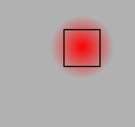
© Government of Canada, Canadian Conservation Institute. CCI 96638-0010
Figure 14. Fuzziness in the boundary between affected and unaffected items.
Description of Figure 14.
The diagram shows a grey rectangle representing the whole asset. Within it is a fuzzy red circle; the colour of its perimeter diminishes gradually to grey. A black line in the shape of a square is placed inside the perimeter of the red circle.
Check if the value pie guides this boundary
Before proceeding further with analyzing B, loss to each affected item, it is helpful to consider the value pie. For example, if there are some high-value items in the scenario which dominate the total value of the affected items, then it will certainly be easier, and much more useful to decision makers, to be sure your boundary captures all the high-value items and not to worry about uncertainty in the low-value items. With the boundary determined by these high-value items, you can return to estimating B, loss of value to each affected item, based on this same boundary.
Aggregating or disaggregating
Analysis of the boundary may prompt you to consider splitting the scenario into two or lumping it in with another one. See the later subsection about aggregating and disaggregating specific risks.
Analyzing B when loss is total
Set B=5
For scenarios that cause total and unambiguous loss of items, such as fire (total combustion) and theft, you can assign B a score of 5 immediately. For these risks, analysis requires only A, the frequency or rate, and C, the items affected.
One can make very precise quantitative comparisons between the risks that cause total loss, since A, frequency or rate, is objective, B, loss of value to each affected item, is also now objective, and C, the items affected score is partly objective.
These kinds of risks, with total loss of items, are the only ones for which the word “risk” was traditionally applied in heritage organizations.
Dividing risks with B=5
In the evaluate step, it can be helpful to divide risks into the two types — total loss and partial loss — so as to make precise comparisons within each group, before comparing all risks together.
When loss is partial: Analysis of the deterioration
Two stages for analyzing B, loss of value to each affected item
The analysis of B, loss of value to each affected item, has two very different stages:
- The analysis of the deterioration
- The analysis of the consequent loss of value
The first is a technical question. The second is a cultural value judgement. Both answers will enter your scenario.
The first stage of the question
What is the description, or an illustration, of the expected deterioration, so that I and others can judge the loss of value?
Do a quick draft to find the source of uncertainty
A useful strategy is to enter your “best guess” about the future deterioration in your notes, e.g. “the light will cause just noticeable fading of all the red in ~10 years” or “the costumes in the open display will be noticeably grey and dirty-looking from pollution in ~10 years.” Use common sense, or conduct short discussions with colleagues. Continue on to the subjective part of the analyze step, the consequent loss of value, and make a first draft of the magnitude of risk scores, with best and worst scores.
This quick draft can establish were you need to focus more effort on refinement of the analysis. For example, it may be that you are much more uncertain about the consequent loss of value due to the fading and the pollution than you are about the rate.
Don’t waste time reducing already low uncertainty
The only way to improve the final risk analysis is to refine the part that is most uncertain. If you cannot improve that part, then there will be negligible benefit to improving the other parts.
If you are analyzing risks of the same kind or using a common criterion for B, loss of value to each affected item, such as just noticeable effect, then you have avoided uncertainty in the subjective part (loss of value) and you can focus usefully on technical refinements.
When loss is partial: From deterioration to loss of value
The subjective stage of the question
Now that you have predicted the deterioration, the question becomes:
How much value will be lost as a consequence of this deterioration?
The context information now comes into play.
Consult the documents
Remind yourself (and those assisting in the judgement) of the organization’s mission statement, its mandate, its various conservation policies, and the “statements of significance” for each item.
In heritage organizations large and small, statements of significance may not exist. In small organizations, even a simple mission statement may not exist. A risk assessment exercise can provide the incentive to create such documents, since it begs the question: Why are we preserving this heritage asset?
Use sample images to calibrate judgements
Try to obtain images of the kind of deterioration you expect. It will be invaluable in both the scoring process and for the decision makers later. Many of us in the field have begun to develop image sequences of various common types of deterioration processes, which will allow us to calibrate B, the loss of value to each affected item, both within an organization and between organizations with similar mandates.
Collect judgements without bias
Appropriate experts and stakeholders, (which may mean just a few colleagues or friends of the organization) can play a large role in establishing B (loss of value to each affected item). To make subjective judgements, i.e. opinions, into a useful “fact” for risk assessment, one needs to compile as many as possible and to do so without biasing them. Be sure to ask individuals to make their initial judgements without knowing what anyone else has stated. Compile their unbiased votes, and only then bring the group together to discuss whether a refinement is possible or not.
Our experience of presenting the same risk scenario to numerous groups of participants and allowing them to vote anonymously has shown that the difference between the highest B score (loss of value to each affected item) and the lowest B score can often be as much as 3. It also shows, however, that given the opportunity for subsequent discussion, the majority will consistently converge on scores that differ only by 1.
Four routes into the score
In this manual, we suggest four routes to finding B (loss of value to each affected item):
- fractions,
- area on a diagram,
- verbal scale, or
- equivalence to total loss.
Only the last one, equivalence, provides a rigorous quantitative answer for use in comparative and comprehensive risk assessments.
These four routes are discussed next.
When loss is partial: Using fractions
Fractions as the basis of the scale
Loss of value to each affected item is simply the refinement of statements of the following type: “If it gets cracked (or chipped, faded, mouse eaten, stained, worn, etc.) like that, it will lose a third of its current value.”
For some items in some heritage assets, a fractional loss of value, or loss of “utility,” can be meaningfully assessed, such as 50%, 10%, 1%. If your organization can develop a schema for establishing fractional loss numerically, document it, and use it.
Such direct estimates of loss of value as a numerical fraction tend to work well for large losses, in the 10% to 100% range. While precision in such numbers is necessary for financial risk purposes, e.g. distinguishing 50% from 30% of market value, it is rarely necessary in a heritage risk assessment for purposes of deciding priorities for preservation activity. The distinctions that matter are order of magnitude — will that chipping, fading, mouse damage, staining, wear, etc. cause 30% loss, or 1%, or 100 times less, 0.01%?
Very small fractions are difficult for us to comprehend. The next three subsections provide alternate paths to B, the loss of value to each affected item.
Software tools
In other fields of risk, quantification of subjective scales relies on software. These process a large set of simple comparisons from the experts or stakeholders, check for consistency, ask for reassessment of inconsistent judgements, and finally calculate a numerical spacing that fits all comparisons.
| B Score | Fraction of value lost in each affected item | Range |
|---|---|---|
5 |
100% |
100% to 60% |
4½ |
30% |
60% to 20% |
4 |
10% |
20% to 6% |
3½ |
3% |
6% to 2% |
3 |
1% |
2% to 0.6% |
2½ |
0.3% |
0.6% to 0.2% |
2 |
0.1% |
0.2% to 0.06% |
1½ |
0.03% |
0.06% to 0.02% |
1 |
0.01% |
0.02% to 0.006% |
½ |
0.003% |
0.006% to 0.002% |
When loss is partial: Using diagrams
The fraction as a graphic
Part of the problem with numerical fractions, especially very small ones, is that few of us, even scientists, have any “feel” for them. Graphic representations of fractions tap into our powerful visual ability to perceive scale directly, without the abstraction of numbers. Such visual metaphors can build bridges to our “feel” of how big, or intense, or significant is the fractional loss of value, without relying on the ambiguity of words.
Create your own graphic scale
Use one sheet of A4 or letter size paper per step. You will need nine pages. Using word processor software or graphic software, make a gray square 20 cm x 20 cm (just fits inside an A4 sheet.) Make white squares within the grey square, offset from the centre, but not exactly in a corner. Use the dimensions in Table 14. Label the B score, the fraction (optional) and the linguistic scale (optional). With current technology, sufficient precision for the full scale down to 0.003% is readily made and printed.
| B Score | Fraction | Size of white square if grey square 20 cm |
|---|---|---|
5 |
100% |
20 cm |
4½ |
30% |
11 cm |
4 |
10% |
6.32 cm |
3½ |
3% |
3.46 cm |
3 |
1% |
2 cm |
2½ |
0.3% |
1.1 cm |
2 |
0.1% |
0.63 cm |
1½ |
0.03% |
0.35 cm |
1 |
0.01% |
0.20 cm |
½ |
0.003% |
0.11 cm |
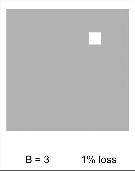
© Government of Canada, Canadian Conservation Institute. CCI 96638-0011
Figure 15. Example of the graphic scale for 1% loss, a B score of 3.
Description of Figure 15.
The diagram represents a standard sheet of paper, letter or A4 size. Covering most but not all of the paper is a gray square. In the top right region of the grey square is a small white square. At the bottom of the figure is the text "B equals 3," and "1% loss."
This is metaphorical, not concrete
When using the graphic scale with others in group work on the B score, emphasize that this is not a concrete representation of a hole in the item. It is a visual metaphor that represents amount of value lost and amount of value remaining. For concrete damage that happens to be a missing piece of the item, the graphic scale may be much larger or much smaller, depending on the value lost.
When loss is partial: Using words
Verbal scales
Verbal scales are commonly used in risk assessment, particularly for communications with stakeholders. Table 15 provides a verbal scale for the B score.
The words of the B scale have been selected judiciously and can be used for heritage risk assessments. In the experience of those who have used this particular verbal scale, when combined with quantitative use of the other two components, it can reliably separate large risks from small risks and provide some guidance on intermediate risks.
Remember that verbal scales are not quantitative. If used for analysis of risk, this must be noted clearly in the report.
| B Score | Definition in words |
|---|---|
5 |
Total or almost total loss of value in each affected item |
4½ |
- |
4 |
Large loss of value in each item affected |
3½ |
- |
3 |
Small loss of value to each item affected |
2½ |
- |
2 |
Tiny loss of value to each item affected |
1½ |
- |
1 |
Trace loss of value to each item affected |
½ |
- |
When loss is partial: Using equivalence to total loss
The equivalence balance
The only rigorous way to arrive at an estimate of partial loss of value is by reformulating the question for B as follows:
How many items could suffer this partial loss of value before the organization would prefer instead to lose just one of the items totally?
For example, if archival paper sheets are made slightly brown by adjacency to the cardboard of standard file boxes, the archivists can be asked for an estimate of equivalence. They may say that given the mandate of the archive, to preserve information, they would prefer to have 10,000 slightly brown sheets rather than a fully destroyed one. From Table 16, the archivist has chosen B score = 1.
On the other hand, a curator of a fine art print collection with 1000 items may estimate that only ~100 prints could be slightly damaged by this kind of browning before the organization would prefer to have one stolen. Here the B score = 3.
Equivalence and fractional loss of value
In Table 13 where B scale was expressed in terms of a fraction (percentage) the score B=3 was 1% loss in value, i.e. 1/100. The score B=3 in Table 16 is expressed as “100 items” that could suffer this degree of partial damage before the organization would prefer to lose one item totally. The two are simply the reciprocal of each other.
| B Score | Number of items with partial loss that equal the total loss of one item | Range |
|---|---|---|
5 |
~1 |
1 – 2 |
4½ |
~3 |
2 – 6 |
4 |
~10 |
6 – 20 |
3½ |
~30 |
20 – 60 |
3 |
~100 |
60 – 200 |
2½ |
~300 |
200 – 600 |
2 |
~1000 |
600 – 2000 |
1½ |
~3000 |
2000 –6000 |
1 |
~10,000 |
6000 – 20,000 |
½ |
~30,000 |
20,000 – 60,000 |
Equivalence is the gold standard for the B score
Equivalence to total loss is not just a way of expressing partial loss, it is the only way to calibrate the measurement of partial loss. No matter whether one has used the verbal scale, the fraction scale, or the graphic scale for partial loss of value, when one gets to the risk evaluation stage, one is in effect using equivalence to say that risk X is greater or smaller than risk Y.
When loss is partial: Equivalence chains
What is an equivalence chain?
An equivalence chain is a series of equivalence judgements between total loss (100%) and the smallest partial loss one needs for the assessment, which perhaps is as small as 0.01% (10,000:1). The ratio between each link in the chain, e.g. 10:1, or 30:1, or 100:1, is much less than the enormous ratio 10,000:1 between the beginning and the end of the chain.
Why use an equivalence chain?
There are two problems with trying to get an accurate feel for a large ratio like 10,000 items versus 1 item. First is our general inability to use large numbers for any subjective decision-making situation. Second is the practical limitation in applying large equivalence ratios to small collections of items. For example, to ask an organization with 500 paintings to imagine an equivalent loss of value based on 10,000 paintings is not simply difficult, it is meaningless.
Equivalence chains can help solve this problem. They not only help the analyst, but also the decision makers. In particular, those who initially reject the whole idea of quantifying partial loss of value may come to accept its application when presented as a concrete chain of comparisons between different degrees of damage.
Making an equivalence chain
Imagine 11 similar items, a single item on one side and a group of 10 on the other side. Imagine that you can choose between two different futures: total loss of the single item or partial damage to each of the group of 10. How much damage would you accept to each of the 10 before you prefer instead the total loss of the single item, e.g. to fire? The partial damage that you imagined represents a 10% loss of value, i.e. a B score of 4 and “a large loss of value” in the verbal scale.
Now repeat the process, but this time imagine that the single item is only damaged to the extent established as 10% loss. How much damage would you accept to each of the 10 before you prefer instead the 10% loss of value to the single item? This partial damage to the 10 items represents a 1% loss of value to each item, i.e. a B score of 3 and “a small loss of value” in the verbal scale.
One can repeat the process to represent B scores of 2 and 1 if needed.
If the exercise seems unreal, keep in mind that whenever one makes decisions that affect risks to the heritage asset, one is in fact choosing between these kinds of futures.
When loss is partial: Value judgements may not be necessary
It isn’t necessary for many risk-based decisions
As noted in the overview of same-risk assessments, one can use risk assessment to make rational prioritization of many classic conservation decisions such as lighting or climate control without confronting the difficult question of how to convert different kinds of deterioration into loss of value.
Set a common loss of value across multiple risks
As noted earlier when discussing A, the frequency or rate score, one can select a criterion for B, loss of value to each affected item that is perceptually the same across many kinds of deterioration, i.e. the lowest observable adverse effect (LOAE). One then fixes the B score for the LOAE, typically 1 (trace) or 2 (small). One can then make quantitative comparisons between all the risks that use the same LOAE criterion. The risk ranking will then depend only on the A and C scores.
Analyzing C if all items have equal value
No value pie needed
If all items that constitute the heritage asset are of equal value, there is no need to explore the value pie. More precisely, we are using a particular form of the value pie, one where each item is given equal value.
Calculating the fraction affected
Count the number of affected items, and divide by the total number of items in the asset.
In this example (Table 17) there are 36 items affected by the scenario and a total of 11,239 items in the collection. The fraction affected is therefore 36/11,239 ≈ 0.0032, or 0.32%, for a C score of 2½.
| Number of items affected | Number of items in the whole asset | % of asset value affected | C Score |
|---|---|---|---|
36 |
~11,239 |
36/11,239 = 0.32% |
2½ |
Analyzing C when items vary in value
The value pie
Recall the first value pie table and graphic introduced in the establish the context step. That value pie table is reproduced in Table 18.
Calculating C with the value pie
The example in Table 18 shows the calculation for a risk where 2 textile treasures and 30 average textiles are affected. The 2 treasures represent 3.4% of the asset value, and the 30 average textiles represent 0.24%, for a total of 3.64%. The C score is 3½ on the 1/2-step scale. Note that removing the 30 “textile, average” items from the calculation would not change the C score at all, but removing the two treasures would reduce the score to 2½ (on the 1/2-step scale).
C score is often the most important to establish carefully
This is an example where establishing whether the items affected include any precious items, and exactly how many, is far more important than establishing high accuracy on the other two scores, A or B. It will also become important in developing and analyzing risk treatment options.
Of course, precious items are often the ones that organizations like to place on display.
Comparison with equal value items
Compare the C score for the same situation, but for which all 11,239 items in the heritage asset have been assigned equal value (previous subsection, Table 17). There the C score was only 2.5, a drop of almost 1.5 points. On the ABC scales, this is a huge difference, representing a factor of 30, because these are order of magnitude scales.
| Group | Group as % of asset | Value subgroup |
Number of items in the value subgroup | Value subgroup as % of its group | Value subgroup as % of the asset | Each item as % of the asset |
|---|---|---|---|---|---|---|
Building |
50% |
Windows |
12 |
40% |
20% |
1.7% |
Building |
50% |
Exterior finish |
1 |
30% |
15% |
15% |
Building |
50% |
Interior finish |
1 |
30% |
15% |
15% |
Collections |
40% |
Textile treasures |
6 |
25% |
10% |
1.7% |
Collections |
40% |
Textiles, average |
1200 |
25% |
10% |
0.008% |
Collections |
40% |
Mixed treasures |
4 |
25% |
10% |
2.5% |
Collections |
40% |
Mixed average |
10,000 |
25% |
10% |
0.001% |
Site |
10% |
Landscape |
1 |
80% |
8% |
8% |
Site |
10% |
Sculptures |
14 |
20% |
2% |
0.14% |
| - | - | - | Asset total = 11,239 |
- | Asset total = 100% |
- |
| Affected items | Each item as % of asset | Number of items affected by this risk | Fraction of asset value affected | C score on 1/2-step scale |
|---|---|---|---|---|
Textile treasures |
1.7% |
2 |
1.7% x 2 = 3.4% |
3½ |
Textiles, average |
0.008% |
30 |
0.008% x 30 = 0.24% |
2½ |
Textiles |
- | 32 |
3.4% + 0.24% = 3.6% |
3½ |
Analyzing a risk by using the probable institutional response
Why look at institutional response?
For rare and catastrophic events, it is well understood that analysis of risk depends in large part on a prediction of institutional response, e.g. are there plans in place to safeguard items prior to impending flooding, or are there plans and materials in place for effective response and recovery after the flood? Institutional response can also provide the key to analysis of slow processes.
The initial analysis
Consider an institution where the majority of the items are in storage (possibly accessible storage). A typical risk arises when such organizations place a few items, often of special value, on public display at the entrance to the building “for window appeal.” Suppose several hazards are known to be much higher there, such as light intensity, the likelihood of theft and vandalism, etc. Let us assume one or all of these risks will happen very soon, estimate within 10 years, so A=4.
Now assume that “fading beyond use” or “vandalism beyond use” will score as almost total loss, so B=5. If it is one item among 10,000 items of equal value, then C=1.
The magnitude of the risk is therefore MR=4+5+1=10, a high risk because A and B are so large.
Adding the knowledge of institutional response
Suppose one has decided to select a long-term time horizon of 100 years for the risk assessment, and one chooses to analyze all cumulative processes on this time horizon. Therefore one sets A=3. Only B, loss of value to each affected item, and C, items affected, are in question. The question now becomes, what is the predicted response of the institution if the item on display is lost or damaged beyond use in 10 years? Will they replace it endlessly as simply the cost of window appeal, or will they treat the risks in that particular situation, by using reproductions, for example?
If they replace endlessly, then items affected (C score) climbs to 2, since 10 items are lost over 100 years, so risk remains at MR=3+5+2=10. If they stop the process after they discover the first item was lost so quickly, then C, items affected, remains only 1, and the magnitude of the risk from the 100 year perspective drops to MR=3+5+1=9.
If the displayed items are more valuable than average
If the items are selected for display on the basis of their significance and represent a much larger portion of the value pie than mere numbers imply, then of course the C score, items affected, will climb. For example, if the item on display is 10 times more valuable than average, then the magnitude of risk in all the examples climbs another point.
Review for coherence in the analysis of the three components
Coherence
Analyzing the three scores A, B, and C one after the other may result in a drift in how one conceives the risk during each step. Perhaps one rethinks A, the frequency or rate, so as to make B, the loss of value to each affected item, more clear, but then fails to adjust C to match. Perhaps one rethinks the boundary of C, items affected, so as to make B, loss of value to each affected item more clear, but fails to adjust A, frequency or rate. Analysis of the three components is an iterative process.
At the end of the analysis, the analysis of the three scores A, B, and C must be coherent with each other.
Sometimes it helps to start with C before A or B
The single most important aspect of coherence overlooked by new users rests on C, i.e. the definition of the items affected. If the boundary around the items affected expands or contracts while conceptualizing A and B, it is essential to check that one has revised C appropriately. One can reduce this error by starting the analysis with C, then moving on to B and A.
Review, review
Not all uncertainty can be eliminated, but substantial reappraisals and refinements of scenarios are not uncommon in midstream.
Finding knowledge
Sources of knowledge
In the Explanations subsection of the identify risks step, we introduced the three sources of knowledge (Table 8) and typical examples of each:
- Regional statistics
- Local knowledge
- Scientific and technical knowledge
Various frameworks needed for understanding risks were also introduced – Agents, Types, Stages, and Layers.
A sequence of collecting information for comprehensive risk assessment — local knowledge, facilities surveys, and regional data — was introduced in the identify risks step.
In the analyze step, we enter a second phase of gathering information from these same sources and thinking about these same frameworks, but this time we are guided on where to focus our efforts by the scores given to the first draft scenarios.
Knowledge phases during risk analysis
Phase 1 — What you know already
Based on what you know already, write a first draft of the likely scenario. Add drafts of the worst and best case scenarios. Score the scenarios (high, probable, and low).
Phase 2 — Research what you don’t know
Find new information for revising scenarios and improving their analysis. Focus on those scenarios where the worst case scenario has a high magnitude of risk score and where uncertainty is large, i.e. where the likely scenario is much lower than the worst case scenario.
Phase 3 — Stop and consult
In our experience, analysis of a single risk can take between one day and one month, depending on whether one has analyzed that kind of risk before. With difficult risks, it may be better to consult with colleagues, stakeholders, and even the decision makers as soon as you have “good enough” estimates (better earlier than later).
Phase 4 — Finalize
Another phase of knowledge gathering may follow after the evaluate risks step, to refine analysis even further, based not only on uncertainty, but also on other issues (some of which may emerge during the process of consultation).
Aggregating and disaggregating specific risks
Be prepared to refine your risk identifications
There is no simple recipe for choosing how specific or non-specific to make each risk. In the identify step, you were given tools for separating risks into groups, by agent and by type. During analysis, you may discover that it makes sense to revise these scenarios to make analysis simpler or more reliable.
Aggregating scenarios to help analysis
It may become obvious during analysis that some scenarios can be merged without increasing the uncertainty. Or they must be merged in order to take advantage of the available facts and theories. Many risks simply do not have enough facts or theories to allow multiple detailed scenarios, even if we can imagine them clearly.
Aggregated risks can also be more useful for “big picture” decisions.
Disaggregating scenarios to help analysis
It can often be quicker to analyze two clear scenarios than one ambiguous one and more useful to detailed decision making.
The process of thinking about the worst case scenario may prompt us to disaggregate a risk, so as to capture the worst case separately. For example, if we think of a fire risk in a work room with a lot of ignition sources, and we think it is likely to be contained in one room, but thinking about worst case prompts us to add the chance the fire will spread to the whole building, it will be more useful to consider two separate scenarios — “fire in the exhibit prep room when items present” (which has a much higher probability, but exposes far fewer collection items) and “fire from the prep room spreading to adjacent collection storage.” Not only does each have very different scores of frequency (A) and items affected (C), the treatment options for reducing each risk are very different.
Facts plus theories: The general method for analyzing scenarios
A general method
Analyzing a scenario is like solving a detective story — one links facts to theories. But you are also the writer of this story…you must place adequate facts and theories in your scenario, so that you can analyze the story.
The first draft of a risk analysis often begins with regional and local historical facts. Then current theory for that agent may (or may not) allow the analysis to be adjusted for your specific scenario (and for your later specific treatment options.)
Facts
Facts are facts. They are not, however, just scientific facts. For events, they are often historical facts: the frequency of earthquakes, the frequency of heritage thefts in the region, the number of items that have been dropped and broken within staff memory, etc.
For cumulative processes of deterioration, scientific facts become more common, but cumulative processes are also informed by the facts of our own experience and our own organization — that some textiles have faded, that newspapers have yellowed, that some negatives have cracked emulsions, that some structures in the site have weathered, that the stairs in a historic house have abraded, etc.
Theories
Theories refer to all the forms of explanation that allow some sort of prediction of risks, from well-established scientific models, such as those for light fading, to the correlations in large sets of facts that allow one to say that some factor can double the risk. The sources of theories are not only the technical and scientific literature, but also our common sense, our imaginations, and our reasoning.
Theory: Exposure to events
Events are usually modelled by a probabilistic model. This means that the initial event, such as an extreme rainfall, has a certain probability, e.g. 1 in 50 years, but that each link in the chain of events that leads to items becoming wet also has a probability.

© Government of Canada, Canadian Conservation Institute. CCI 96638-0013
Figure 16. Frequency diagram of the chain of events for two different levels of control of an external hazard such as rain water.
Description of Figure 16.
From top to bottom, four rectangles represent: 1) the probability of roof leakage, 2) the probability of water hitting a case, 3) the probability that the case leaks, and 4) the final frequency of items becoming wet in each scenario.
The probability that a well-designed roof in good condition will leak somewhere during that extreme rainfall might be 1 in 10. If the display cases containing collection items cover half the floor under that roof, then the probability of a case somewhere catching the leak is 1 in 2. If the cases are well-designed water-shedding cases, the probability of the case allowing water inside might be only 1 in 50 cases.
The overall probability that an extreme rainfall will result in wet items inside one display case is simply the product of this chain of probabilities:
1/50 y x 1/10 x 1/2 x 1/50 = 1/50,000 y.
In another building, the roof is so poorly designed it is guaranteed to leak for such an extreme rainfall, and the cases do not shed water, so the probability of a case getting wet is five hundred times higher:
1/50 y x 1 x 1/2 x 1 = 1/100 y.
If the roof is expected to leak in 10 places at the same time, the items affected is another 10 times higher as well!
If you are lucky, you can avoid all these calculations and just use local knowledge, such as “in the last twenty years we get at least one small roof leak every rainy season in the storage area.”
Theory: Exposure to cumulative processes
The cumulative process agents, and many common event agents, are usually modelled by some form of flux model, sometimes called “kinetic,” or “flow,” or “transmittance” models. This simply means that there is a movement of the agent (gas, light, heat, moisture, bugs, abrasive forces, etc.) from the source towards the heritage asset.
In Figure 17, daylight is followed from the known outdoor average of 30,000 lux through two different scenario paths. The final flux, or exposure, is the product of the intermediate factors. (“Daylight factor” equals the ratio of the window or skylight area to the room area). This exposure, in combination with the item’s sensitivity, can be used to calculate an effect, such as fading.
In the example of Figure 17, the risk is being analyzed by selecting a particular degree of damage, in this case the total fade of sensitive colorants (ISO#1 and #2). This dose is known to be ~30 Mlxh (megalux hours). With the dose per year of each scenario calculated, one can then find the A score, i.e. the time to reach that selected damage.
Within the framework of the five stages of control, flux models allow us to quantify the block stage but also the avoid stage, inasmuch as reduced display time is avoidance of daylight.
(Often, of course, it is simpler just to measure the exposure to light, or pollutants, or pests, etc., at the item directly.)
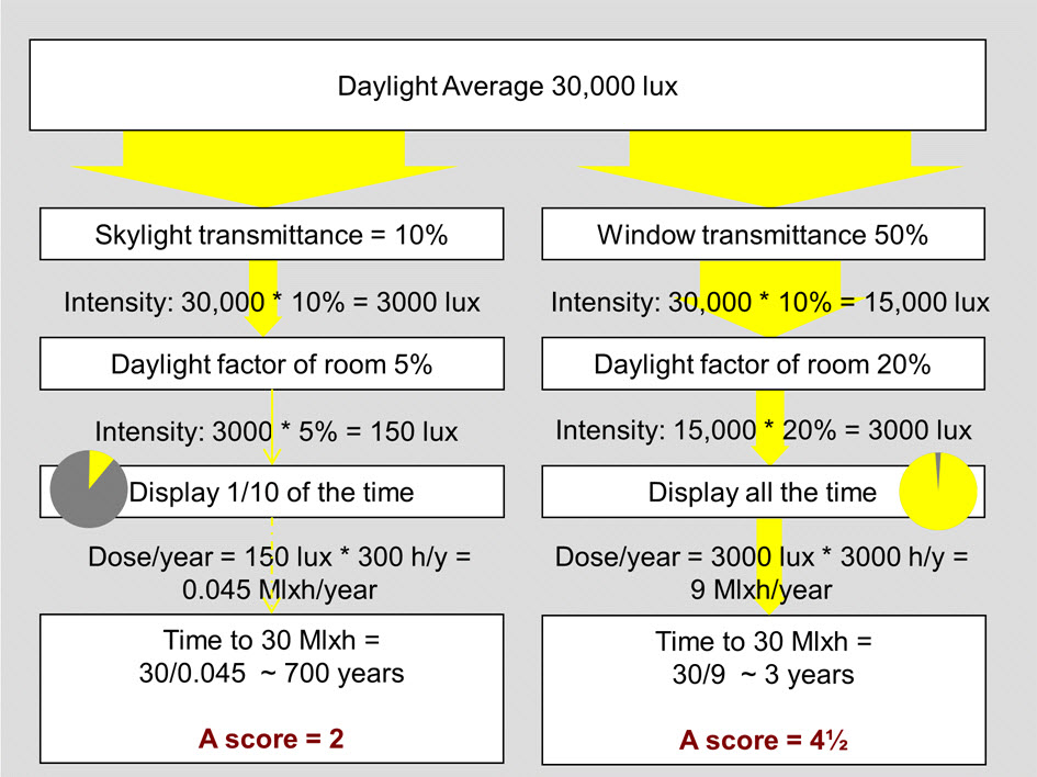
© Government of Canada, Canadian Conservation Institute. CCI 96638-0015
Figure 17. A flux model for the cumulative process of light fading.
Description of Figure 17.
From top to bottom, four rectangles represent: 1) the transmittance of windows or skylights; 2) the daylight factor of the room; 3) the display schedule (fraction of the year on display); and 4) the final calculation of years to reach the required dose to cause the selected damage.
Analyzing risks by control levels
Sometimes theories are unavailable
Some risks are too complex to be analyzed by a simple theory such as those for fading by daylight and damage by roof leaks (described in the previous sections). Theories may exist but be impractical to use or incomplete.
Control level approach
For risk purposes, one needs a list of indicators that correlate to different levels of risk. This has been achieved for two agents of deterioration: fire (Tetreault, 2008) and pests (Strang and Kigawa, 2013). Rather than call them levels of risk, they are optimistically called levels of control.
| Control level | Examples of indicators (NOT a complete list) | Average time between events | Initial object only | Room only | Floor only | Whole building |
|---|---|---|---|---|---|---|
1 |
Detectors |
140 yr |
28% |
29% |
17% |
26% |
2 |
Resistant walls |
140 yr |
28% |
34% |
19% |
19% |
3 |
Fire doors |
160 yr |
42% |
56% |
2% |
0.07% |
4 |
Sprinklers in storage |
720 yr |
53% |
46% |
1% |
0.01% |
5 |
Specialized staff |
1500 yr |
68% |
31% |
1% |
0.006% |
6 |
Sprinklers everywhere |
2800 yr |
99% |
2% |
0.02% |
0.001% |
Fire control levels
Table 20 summarizes the control levels for fires in Canadian museums. For example, museums at control level 1 can expect a fire event per museum every 140 years, of which 26% will spread to the whole building (so the probability of a total building fire is once every 540 years). The table was developed by combining ten years of historical data on fires in Canadian museums with the advice of fire experts. For the full lists of indicators, data on where and why fires start in museums, and comparisons with data from other countries, refer to the original article, Fire Risk Assessment for Collections in Museums.
Pest control levels
Table 21 summarizes the control levels for pests. It provides an estimate for the A score in terms of the time for damage to appear in the case of constant exposure to pests, or the time between pest events as exposure decreases. For details on damage by different pests as well as risk reduction methods for each type of enclosure, refer to Agent of Deterioration: Pests.
| Control level | Type of covering or building | Time for noticeable damage to appear or time between events (Robust, soft, or delicate materials) |
|---|---|---|
0 |
Outdoors |
Robust – years; delicate – days |
1 |
Roof or tarp |
Robust – decades; soft – years; delicate – months |
2 |
Roof, walls, and loose-fitting doors |
Robust – century; soft – decade; delicate – year |
3 |
Basic habitation |
Robust – life of the building; soft – decades to century; delicate – years |
4 |
Adapted commercial building |
Robust – life of the building; soft – century; delicate – decades |
5 |
Purpose built building |
Robust and soft – life of the building; delicate – century |
6 |
Preservation designed building |
All – minimal over the life of the building |
Don’t ignore local history entirely
Pest risk varies greatly with the six layers of enclosure, the type of collection, and current practices. Thirty years of local knowledge can refine estimates of both frequency and extent of pest events. Similarly, a history of small fires or “near-miss” events can refine fire risk analysis, but only to raise estimates from the control level method, not to diminish them, since frequencies lower than once in 140 years are too low to emerge in local knowledge.
Can we predict the future?
Yes and no
“Prediction is very difficult, especially about the future.”
—Niels Bohr, quantum physicist
“The consequences of our actions are so complicated, so diverse, that predicting the future is a very difficult business indeed.”
—J. K. Rowling, Harry Potter and the Prisoner of Azkaban
“When in doubt, predict that the present trend will continue.”
—Merkin’s Maxim
Induction
Risk analysis depends on what is called inductive reasoning — the commonsensical logic that if the last few travelling exhibits have resulted in at least one painting being slightly damaged each time, then the next few travelling exhibits will likely result in similar damage, unless something relevant changes, e.g. we treat the risk. A great deal has been written in philosophy, in science, and in human comedy about this imperfect but necessary and universal form of reasoning.
Common sense
For our purposes, we will rely on the inductive reasoning of our common sense — the belief that yes, we can predict that the next travelling exhibition will likely cause similar damage to the previous ones, unless we change something relevant. The key words are “likely” and “relevant.”
In summary, risk analysis depends on a belief that we can predict the future to a useful and practical degree and that such predictions will support wise decisions.
The future will be different in some ways
This is not to say that we presume that the future will be just like the past. In many organizations, imagining “future-shock” scenarios are the central focus of their risk management. Heritage advisory agencies are beginning to consider changes in risk estimates due to global warming, such as peak rainfall intensity, the frequency of violent tornados, and rising sea levels.
Making deductions from the evidence of past adverse effects
What can the heritage asset teach us?
It is obvious that the heritage asset itself is a source of local historical data about risks to itself. For example, if it is covered in dust, then maybe we have a dust problem. The danger in our profession has been the assumption that the asset informs us in a simple manner about its future risks via its current state. For example, the furniture is cracked, therefore the risk of RH fluctuations is high, and thus we need a risk treatment such as climate control. Or, nothing in my asset shows fire damage or water damage, therefore there is no fire or flood risk. Such deductions are false.
Our assets delude us about rare risks
Rare and catastrophic risks are a matter of chance. The very fact that we can see our assets in front of us makes us believe that our good luck will continue forever. It is too easy to forget about doing something about the bad locks that haven’t been broken yet, the pipes that haven’t leaked yet, or preparing for the bad storm that hasn’t happened in the last few decades. It is easier to dwell on dust and relative humidity.
Our assets delude us about old losses
Simply surveying an asset does not make us aware of all the items that have been stolen, smashed, eroded, or otherwise lost in the past. Today’s asset can often give the illusion of completeness.
Why do we feel the asset can tell us everything?
The visible and the concrete have a powerful hold on us, especially for many drawn to, and trained in, tangible heritage. Our trained “eye” is so subtle, we begin to rely on it entirely. While interpretation of the remaining material assets is useful, we must not forget that there are many other, perhaps even more important sources of knowledge to guide us. We will not know which knowledge was most useful until the assessment is over and we evaluate the risks we find.
Separating the technical issues from the subjective issues during the analyze step
Studies from other fields
Studies of successful risk assessment projects in other fields of public trust have shown that it is essential to keep a clear distinction between the technical components of risk analysis and the subjective components, i.e. the value judgements. Stakeholders and decision makers will trust experts to provide the best technical analysis (in fact, they demand it), but they want to make the transformation of that technical analysis into a loss of value analysis for themselves.
In other words, when doing the method of this manual, the B score, loss of value to each affected item, will always require the input of appropriate stakeholders. At the very least, any assessment report needs to provide a clear description of the two stages in derivation of the B score, loss of value to each affected item — the expected damage in technical terms, followed by the consequential loss of value.
This distinction is not always sharp, and there will be an overlap in roles. For some assets, experts such as curators are essential for guiding both technical and loss of value judgements, since they may understand the physical nature of their assets, as well as the utility or value of the assets, better than anyone. Even so, it is useful to keep clear where the expert opinion about damage ends and the expert opinion of its impact on value begins, since later examination of this divide during the evaluate risks step is inevitable.
The arithmetic behind the ABC scores
Do I need to know this?
No, you can do the method without the information here. This section is provided for those who want to create their own spreadsheet or database tool, or who want to calculate scores precisely (decimals rather than nearest half).
The arithmetic
The ABC scales are all base-10 logarithms of the components underlying A, B, and C scores, shifted to give a 5-point score for the maximum values selected. Risk in linear units is calculated by taking the product of these underlying components. Since the A, B, and C scores are logarithms of these components, one only needs to add them to obtain the logarithmic expression of risk, i.e. MR.
A scale
= 5 – log base 10 (years between events or years for the process to cause the specified loss).
Thus a time of 1 year between events scores 5; 100 years scores 3; 100,000 years scores 0. Note that a score of “0” does not mean zero frequency; it means a very small frequency.
B scale
= 5 + log base 10 (fractional loss).
Thus total loss (100%) scores 5; 1% loss, i.e. 1/100, scores 3; 1 in 100,000 scores 0; 1 ppm (1 in 1,000,000) scores -1, etc. Note that B is based on fractional loss, not fraction remaining.
C scale
= 5 + log base 10 (fraction of heritage asset affected).
Thus 100% of asset affected scores 5; 1% of asset affected scores 3; 1 in 100,000 scores 0; 1 ppm scores -1, etc.
Negative Scores
Recall that MR = A + B + C
Normally, if one of the A, B, or C scores drops to 0 or less, the procedure is simply to ignore the risk entirely, but if one prefers, one can keep the negative numbers and calculate MR. The MR value can then go below 10 even if two of the scores are already 5 each. This can be useful in large museums with over a million items or for extremely rare events. Risks scoring below MR 10 will rarely be priorities, but it may be of interest to place them accurately relative to other risks.
Risk on linear scales
“Linear scale” simply means the type of scale with which we are all familiar, without logarithms. In any formal equations, when we use the expression “Risk” as opposed to “Magnitude of Risk” we will imply the linear scale, and we will note the units: “fraction of asset value lost per year.”
Risk = fraction of asset lost per year = 10 ^ (MR - 15).
MR = 15 + log base 10 (fraction of asset loss per year).
Thus the top score, MR 15, is the risk of 100% asset loss in 1 year. MR 13 is a risk of 1% (1/100) asset loss per year; MR 10 is a risk of 1/100,000 asset loss per year, etc. One can choose to express loss per century or any other period of time.
Step 4: Evaluate Risks
Risk evaluation is the process that leads to an evaluation of each specific risk relative to other risks or to some criteria.
Task 1: Compare risks to each other, to criteria, to expectations.
Task 2. Evaluate the sensitivity of prioritization to changes in the value pie.
Task 3: Evaluate uncertainty, constraints, opportunities.
Tasks for the evaluate risks step
Task 1: Compare risks to each other, to criteria, to expectations
Compare risks to each other by MR
Sort the risks by MR, from highest to lowest. Using the CCI database, or spreadsheet software, or graphing software, make a bar graph of the sorted MR values, labelled with the risk names. Sorted horizontal bar graphs are called “tornado” graphs, due to their appearance. The priority risks are the big bars at the top of the tornado. This tornado graph of MR is the most important means of risk evaluation in this method.
A stacked bar graph of the A, B, and C scores allows one to see both MR and the component contributions. (See Explanations for an example.)
Compare each risk to the MR Scale with Implications
In Table 23, the range from MR 5½ to MR 15 has been divided into five bands, each 1½ steps wide. Traffic light colours and titles of “Catastrophic Priority,” “Extreme Priority,” “High Priority,” “Medium Priority,” and “Negligible Priority” have been assigned to these ranges, based on an estimate of what a major national organization with a preservation mandate of 100 years or longer would probably expect of itself.
Between 2010 and 2015, CCI assessments of several museums, galleries, and archives suggest that out of approximately 25–40 specific risks analyzed for each organization, there were always a few large risks which warranted special attention in the executive summary of the report. We observed that these short lists of largest risks were above MR 10.
Use a criterion of “acceptable” risk
It is very useful for an organization to decide that reducing risks below a certain magnitude is simply not worth any effort, i.e. that such risks are acceptable. Actually, the term “acceptable” is misleading; what the organization means is that it accepts small risks because it has bigger risks to address first.
Compare loss to a technical criterion
Single-risk assessments, such as light damage or error rate in digital records, may have a predetermined criterion of acceptable and unacceptable loss to each item. These criteria enter the risk analyses in terms of the B score, loss of value to each affected item. In some cases, for example digital records, such criteria can define total loss of value.
Compare risks to expectations
An important goal of risk assessment, as compared to traditional preventive conservation, is the correction of false expectations, in particular:
- Large risks that were previously unrecognized
- Small risks that were previously exaggerated
Identify these surprises and develop discussions for communication with the organization.
Task 2. Evaluate the sensitivity of prioritization to changes in the value pie
Recognize and communicate the issue
Some users and assessors will be suspicious that the value pie is being used to manipulate prioritization of risks. In fact, the value pie is being used to weight prioritization towards the more valuable parts of the heritage asset. If necessary, explain the role of the value pie and the fact that it can be adjusted by the organization at any time.
Recognize sensitivity as a useful form of evaluation, rather than a problem
In sensitivity analysis, one looks for the specific judgements which make big changes in the final order of risks for only small changes in the judgement of relative value. Of course, sometimes it is obvious to determine which judgements will “drive” which priorities, but experience in other fields of risk analysis shows that it is not always the case.
Use the value pie to illustrate sensitivity
If there is a range of opinions about how the value pie should be divided, or curiosity about its role in the prioritization of risks, make changes in the value pie ratios as needed, and recalculate the MR of all risks (automated in the CCI Risk Management Database). Generate the MR tornado graph for each change in the value pie, and compare.
Use extreme value pie changes to illustrate the role in general of the value pie.
Recognize that the highest risks tend to be less sensitive to the value pie
In practice, the largest risks are less sensitive to the value pie settings because risks such as total fire and severe earthquake affect all items in the heritage asset similarly.
Identify where sensitivity arises in the value pie
If a significant change in prioritization occurs with changes in the value pie, identify which item group is responsible, and communicate to the organization. This helps direct their attention to the review and refinement of the value pie where it is useful to do so.
Task 3: Evaluate uncertainty, constraints, opportunities
The MR versus Uncertainty Table
Sort the risks into a 2x2 table as shown below:
| Low uncertainty | High uncertainty | |
|---|---|---|
| High MR | Treat ASAP | Review ASAP |
| Low MR | No action | Review later |
Divide MR into high and low categories using a preselected criterion such as MR 10 or MR 11, or use whatever criterion divides all the risks you have analyzed into two similar size groups. Divide uncertainty similarly. The appropriate response to each of the four quadrants is shown. (ASAP is as soon as possible.)
Review legal constraints
Reconsider the legal context discussed under the establish the context step.
Risks for which treatment decisions will extend beyond your organization's sphere of legal authority may be given lower priority in relation to others of similar magnitudes that can be treated without having to go through cumbersome regulatory or legal processes.
Review the financial constraints
Reconsider the financial context discussed under the establish the context step.
The organization's operational capacity and the amount of financial resources available will probably limit the number of risks that can be treated at a given point in time, even if they all have equally high priority for treatment. External grants and/or internal funds might be available for a limited amount of time and only for specific purposes (e.g. building maintenance, collection registration or shelving/packaging).
These opportunity-driven priorities to treat risks will not necessarily coincide with those established on the basis of magnitudes and uncertainties, so it is important to check them against each other before deciding on which to treat.
Review stakeholder perceptions
The perception and tolerability of risks by the public and other stakeholders can also become a significant contextual factor affecting the prioritization of treatments, especially when sensitive social or environmental issues are involved.
Review staff perception
Sometimes it might be helpful to address risks that despite having lower magnitudes can be easily treated. This will give the team responsible for the risk-based task a sense of accomplishment and will increase their motivation to continue with risk management.
Look for linkages between risks
When two or more risks have a common cause, e.g. the same hazard or the same path followed by the agent of deterioration, or a common factor, e.g. the lack of a given procedure, they can be given preference for treatment in relation to other risks of similar magnitudes showing no such commonalities.
Explanations for the evaluate risks step
An example of a magnitude graph
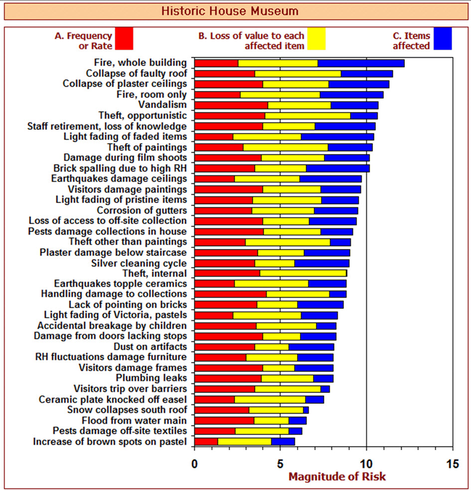
© Government of Canada, Canadian Conservation Institute. CCI 96638-0017
Figure 18. An example of a “tornado graph” from a comprehensive risk assessment. The risks are sorted by Magnitude of Risk or Deterioration from largest to smallest. The A score is shown in red, the B score in yellow, and the C score in blue.
Description of Figure 18.
Each bar is labelled with the name of the risk or deterioration process it represents. The X axis is the magnitude of each bar. There are 37 bars, sorted by magnitude, largest at the top, hence the shape suggested by the stacked bars is that of a tornado or funnel. Each bar has a red portion representing the A score, a yellow section representing the B score, and a blue section representing the C score.
Magnitude of risk scale with implications
| Magnitude of Risk | General Implications of the Range | Colour |
|---|---|---|
15 – 13½ |
Catastrophic Priority: |
red |
13 – 11½ |
Extreme Priority. |
amber |
11 – 9½ |
High Priority. |
yellow |
9 – 7½ |
Medium Priority. |
green |
7 – 5½ |
Negligible Priority. |
blue |
The Magnitude of Risk versus Uncertainty Table
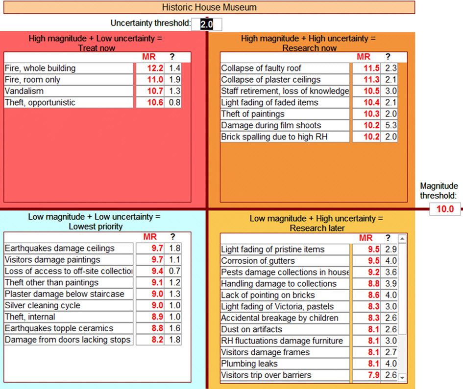
© Government of Canada, Canadian Conservation Institute. CCI 96638-0019
Figure 19. An example of an MR versus Uncertainty table. Top left quadrant, high magnitude low uncertainty: Treat these risks as soon as possible. Top right quadrant, high magnitude high uncertainty: Review and improve the analyses of these risks as soon as possible. Bottom right quadrant, low magnitude high uncertainty: Review and improve the analyses of these risks if and when high magnitude risks have been addressed. Bottom left quadrant, low magnitude low uncertainty: No review necessary, lowest priority for treatment.
Description of Figure 19.
There are four quadrants, each containing a table of between 4 and 12 named risks and their magnitude and uncertainty scores. The significance of these four tables is fully explained in the caption.
Discussing the influence of the value pie on prioritization
The critique of value judgements in this method
In analyzing risk in this method, some components depend only on technical data, such as frequency and rate, and degree of damage. Other components, however, depend on value judgements. A common reaction among those new to the approach is the conviction that these value judgements are arbitrary, or even meaningless, and that they are used to manipulate prioritization. This is a common reaction in other risk assessment fields too, such as human health, where judgements on the meaning of “quality of life” are open to debate.
Judgements must be communal
We are not, in fact, suggesting that the assessor makes the value judgements needed for this method in isolation. The value pie is an organization’s communal judgement, usually dominated by curatorial expertise and taking into account its mandate.
The value judgements are relative, not absolute
The value pie and the B score, loss of value to each affected item, require only relative judgements within the organization, not absolute valuations within a global context.
Reframing the issue as sensitivity analysis
After analysis is complete and evaluation begins, one is in a position to test the sensitivity of the prioritization to the value pie. First, check the sensitivity of the top three to five risks. In practice, one finds that these largest risks, such as fire and severe earthquake, are often unaffected by the value pie because they affect almost everything equally, at which point the division of value within the asset is irrelevant. It is important to communicate to the organization whenever the top priorities are unaffected by the value pie judgements.
Next, watch the ranking of the middle and low risks in the MR graph as the value pie factors are switched between extremes in opinion. Some will change order, some will not.
In conclusion
Look for lack of sensitivity first, since this reduces the anxiety about the value pie. On the other hand, uncover and communicate areas of sensitivity, since these will guide useful review of the value pie judgements.
Working backwards from MR to value pie
Working backwards is OK
In effect, one can revise the value judgements to get the risk ordering one “expects.” Working backwards like this is not necessarily a bad thing; it can be considered an independent way of checking the value judgements. The sole purpose of the value judgements, after all, is to enable risk measurement, so if the final risk measurements “feel wrong” and the hard data parts are correct, that leaves the value judgements open to question.
But test for consistency in reasoning
If, however, such revised judgements contradict reasonable judgements obtained by other paths, the analyst must assist the organization to be self-consistent. If an organization is convinced that a wear-and-tear risk is just as important as an obvious fire risk, then they will have to accept that they consider damage from 30 years of wear and tear is more or less equal to total loss. With that kind of bias, rational risk management becomes impossible.
Step 5: Treat Risks
Risk treatment is the planning and implementation of risk reduction.
Task 1: Identify risk treatment options.
Task 2: Quantify risk reduction options.
Task 3: Evaluate risk reduction options.
An external consultant’s task may end here.
Task 4: Plan and implement selected options.
One cycle of risk management is now completed.
Tasks for the treat risks step
Task 1: Identify risk treatment options
Select the type of treatment
In the field of risk management in general, there are three groups of risk treatment:
- risk transference
- risk acceptance
- risk reduction
In this method we focus on the last two, risk acceptance and risk reduction. Risk transference, i.e. the purchase of insurance or the use of indemnification programs offered by government agencies, is beyond the scope of this method, but it must be considered by the organization when considering financial implications of some risks.
Select the risks to reduce
The first selection of risks to reduce has been made during the evaluate risks step, i.e. one has compared risks to some criterion and divided them into acceptable and unacceptable risks. The treat risk step, however, uncovers two more criteria that will influence final evaluation of which risks to reduce:
- the cost-effectiveness of options
- the cost of options
For risks that are acceptable but borderline, it is useful to develop and assess options anyway in case some are very cost effective.
Invent or discover risk reduction options
- Use the layers and stages matrix (Table 24)
- Consult with experts
- Brainstorm with colleagues
- Look for magnifying and reducing factors in each specific risk
Write the option summary
For each option, write a clear option summary of only one or two sentences.
Estimate option costs
Estimate the initial costs (capital) and the annual costs (operating and maintenance) to implement each option. Remember that annual costs include labour. If you have an option that “costs nothing” but depends on labour, estimate the number of hours per year for the task, including management tasks such as enacting the option, and then estimate the annual cost based on an approximate salary.
Task 2: Quantify risk reduction options
Quantify residual risk
Quantification of the benefits of an option is achieved by quantifying the risk that will remain if the option is implemented. It repeats the analyze risks step, but now you imagine that the option has been implemented.
Develop the option
Specify the option in sufficient detail that it can be used to begin the quantification of its effects on the risk. This is an iterative process in conjunction with the analysis of residual risk described next.
Analyze residual A, frequency or rate
If the original risk was analyzed in terms of a fixed time period, or the time horizon, then options do not change this score. The frequency of most natural hazards cannot change either.
Otherwise, estimate how much implementation of the option will increase the mean time between events or the time to reach a specified degree of damage.
Analyze residual B, loss of value to each affected item
If the original risk was analyzed in terms of a defined degree of damage, this is unchanged by any options.
Otherwise, analyze the physical damage that will still occur even if the option is implemented. Now analyze the loss of value to each affected item that results from this degree of damage.
Analyze residual C, items affected in terms of the value pie
Estimate which items will still be affected even after implementation of the option.
Calculate the residual MR
The new MR, based on the sum of the new A, B, and C scores, is the MR of the residual risk if the option is implemented.
When the reduction is perfect
If the option removes all risk, it is not possible to use the A, B, or C scores, since they are not designed to express a complete absence of risk. Simply assign MR=0.
Provide high and low estimates
As well as the estimate of the probable scores for A, B, and C, provide a high estimate and a low estimate for each score. If in doubt, use the same proportional uncertainty as in the original risk.
Communicate your reasoning and sources
Write clear explanations of how you developed your estimates of residual risk, and cite all sources of knowledge used, especially any quantities used in the reasoning.
Task 3: Evaluate risk reduction options
How much does it reduce risk?
The primary criterion for any option is that it actually reduces most, if not all, of the risk it is aimed at. If one does not have the time or resources to perform a full analysis of residual risk as outlined in Task 2 (previous section) then make a qualitative judgement such as “all, most, or some” risk reduction.
Does it reduce other risks?
Identify options that can reduce multiple risks. The most extreme example is a building replacement. In such cases, one could estimate its effect on every specific risk, but it is sufficient to estimate its effect on only the few biggest risks. If it does not reduce these dominant risks, it cannot be claimed to be an improvement for preservation.
Is it feasible?
Check that the option respects existing laws and regulations concerning the organization and the heritage asset.
Check that it conforms to your socio-cultural and/or spiritual context.
Keep it within feasible budgets, or suggest new sources of funding.
Is it sustainable?
There are many cases of museums finding grants to build elaborate buildings but not finding operating funds to maintain them. Sustainability also includes energy consumption, carbon footprint, and the environment. Consider options that take advantage of government subsidies that reward sustainability.
What is its annual cost?
Although more complex business models can be used, a useful approximation for the purposes of our method is:
(Annual operating and maintenance cost) + (Capital costs/time horizon).
Note that the selection of the time horizon greatly influences annual cost since it spreads out any capital costs.
What is its cost-effectiveness?
Cost-effectiveness is the amount of risk reduced per unit cost. With limited resources, one wants to maximize this. Cost-effectiveness and the reduction in MR are the two most important criteria for evaluation of options. Two methods are provided for this calculation in the Explanations subsection — one simple, one precise.
Does it create new risks?
Options are never without side effects, which may become collateral risks. One of the extreme but all too common examples is a new building that reduces risks such as fire and theft but increases light fading, internal pollutants, or even water hazards. A more subtle example is improvements in emergency doorways to allow rapid human egress as well as rapid evacuation of collections when necessary but creates a new risk of theft.
Task 4: Plan and implement selected options
Normal project management
Planning and implementation of risk reduction options is just another form of project management. It is not the scope of this manual to cover that ground.
Context and communication
While the implementation of some actions will be straightforward, others will probably require the involvement of different layers of management inside and sometimes outside the organization. Understanding of this context in which risks are being managed is important for the successful implementation of your risk treatment plan.
Even more important is that risk treatment plans be fully integrated within the overall management and budgetary processes of the organization. Communication is particularly important in the implementation of risk treatment plans because this is when concrete changes take place in the organization, which need to be clearly understood and supported at all levels.
Explanations of the treat risk step
Developing options: Types of risk treatment
Treatment means lowering your organization’s risk
Risk treatment options typically consist of actions to lower the magnitude of risks to acceptable levels by reducing their frequency, rate, or their consequence.
Treatment can mean risk transference
When an organization pays for an insurance policy, it is transferring specific risks to the insurance company, e.g. the cost of replacement of the building after a fire. Risk transference presumes that items are replaceable. This is not usually the case for heritage items and certainly not the case for the highest value items in an asset.
Treatment can mean risk acceptance
Some risks will be accepted by the organization. This comes about for three reasons:
- The risks have been assessed and are within the organization’s criterion for acceptable risk.
- The risks have been assessed and are above the organization’s criterion for acceptable risk, but there is no known feasible means of further risk reduction.
- The risks are unidentified, so these risks have been accepted without recognition by the organization.
The purpose of comprehensive risk assessment is to ensure that all risk acceptance is in the first two categories — known risks — and not in the third category — unknown risks.
Developing options: Creation processes
Communicate and consult
Develop options as a group. Benefit from the diversity of experiences, expertise, and creative potential of colleagues from different parts of your organization and beyond, for example, conservators, managers, building engineers, conservation scientists, security experts, etc.
Brainstorm
Brainstorming sessions with up to 10 people including core members of the risk-based task team and other key participants are a productive way to develop risk treatment options.
Developing options: The Layers and Stages Matrix
| Stage | Region | Site | Building | Collection Room | Fittings | Packaging, Supports |
|---|---|---|---|---|---|---|
Avoid |
- | - | - | - | - | - |
Block |
- | - | - | - | - | - |
Detect |
- | - | - | - | - | - |
Respond |
- | - | - | - | - | - |
Recover |
- | - | - | - | - | - |
A tool to guide option development
The two conceptual tools used in identification of risks — stages and layers — can be used together to stimulate ideas for treatment options. Table 24 above shows the matrix structure. You fill in the blanks with preliminary ideas. Nothing is too “unreasonable” during brainstorming of this matrix. Its purpose is to enable lateral thinking as much as linear thinking.
Options include procedures
Although the layers are geographic and concrete — site, building, rooms, etc. — the cells of the matrix can include elements that are not concrete, such as organizational procedures, staffing, etc. Insert such ideas in the cell that seems closest to their implementation, for example, a Detect idea at the Building layer would be to increase interior security staff. Night-time security contractors, or video cameras, to watch the building perimeter could be placed either under the Building layer or the Site layer. It is not important if the fit is exact, the purpose of the matrix is to prompt ideas, not restrict them.
Do one matrix for each risk
For each specific risk to be treated, think systematically about missing or inadequate stages of control that could be introduced or improved at each layer. Use the available knowledge about preventive conservation and all the relevant information you have already compiled in your analysis for developing treatment options.
Look across matrices to find commonalities
Once you have assembled brief notes in a matrix for each specific risk being considered, lay out the sheets side by side and look for common ideas, complementary options, as well as redundant options and conflicting options.
Make a list of options
Develop a list of plausible options. Proceed to measuring cost-effectiveness, and then you can compile everything in the Option Summary Table (Table 26).
Complex options
Multiple options for one risk
In some cases it might take a combination of two or more treatment options to reduce risks to acceptable levels. For instance, to reduce risk from pests, the combination of (i) the elimination of pest attractants (avoid), (ii) the sealing of all points of entry in the collection areas (block), and (iii) the frequent monitoring of pests (detect) to enable a fast response if necessary can be effective and sustainable. In other words, the actual “option” is the introduction of integrated pest management.
For purposes of the Options Summary Table (Table 26) and for cost-effectiveness calculations, the best understanding will emerge by considering each option alone as well as considering the “combination” option as a distinct option. It may well be that the organization decides to implement the combination option in stages, so they need to decide what sequence of implementation makes the most sense.
It may also be that components of the complex option are beneficial to other risks, e.g. packaging that reduces insect attack can also reduce other risks.
Cost-effectiveness calculation, simple
An order of magnitude calculation
This simple calculation assumes that the option is effective enough that the residual MR is at least 1 full point lower than the original MR. If this is not the case, one must use the precise method of the following subsection.
Annual cost
Annual cost is calculated by spreading the initial capital cost over the time horizon, then adding the annual maintenance cost:
Annual Cost = Capital cost/time horizon + maintenance cost per year
This annual cost is converted to the magnitude of annual cost (MAC) using the conversion table (Table 25).
Cost-effectiveness
The magnitude of cost-effectiveness is obtained by subtracting the magnitude of the annual cost from the magnitude of the original risk. So:
Magnitude of Cost-effectiveness (MCE) is MCE ≈ MR (original) – MAC
The following two worked examples illustrate the calculation.
Discussion of the worked examples
The examples compare a low-price option (small repairs) that solves a small risk to a high-price option (a new facility) that addresses a large risk. The magnitude of cost-effectiveness of the high-price option is MCE 7, one full point higher than the MCE 6 of the low-price option. Recall that one unit on a magnitude scale is a factor of 10 in linear units, so the new facility option is ten times better than the small repair option. This is a common dilemma in risk treatment decisions: the choice between “feasible” options, some of which have poor cost-effectiveness, versus high-price options which are “beyond our budget” but which may have excellent cost-effectiveness.
Low-price option
This option addresses a small specific risk but requires little cash, modest labour. Initial capital cost of $1,000, spread over 30 years, plus an annual labour cost of $3,000, so annual cost is $33 + $3,000 = $3,033.
Magnitude of Annual Cost, MAC 3½
Original risk before option: MR 9½
Assuming that the residual MR after the option is implemented will be at least 1 point less, i.e. MR<8½, then Magnitude of Cost-effectiveness,
MCE ≈ MR – MAC = 9½ – 3½ = 6
High-price option
One-time capital cost of $30M spread over 30 years, maintenance costs same as current facility, so additional annual cost is $1M.
Magnitude of Annual Cost: MAC 6
Original risk before option: MR 13
Assuming that the residual MR after the option is implemented will be at least 1 point less, i.e. MR<12, then Magnitude of Cost-effectiveness:
MCE ≈ MR – MAC = 13 – 6 = 7
| Annual Cost (in local currency) |
Magnitude of Annual Cost |
|---|---|
10 |
1 |
30 |
1½ |
100 |
2 |
300 |
2½ |
1000 |
3 |
3000 |
3½ |
10,000 |
4 |
30,000 |
4½ |
100,000 |
5 |
300,000 |
5½ |
1,000,000 |
6 |
3,000,000 |
6½ |
10,000,000 |
7 |
30,000,000 |
7½ |
100,000,000 |
8 |
300,000,000 |
8½ |
1,000,000,000 |
9 |
3,000,000,000 |
9½ |
10,000,000,000 |
10 |
Cost-effectiveness calculation, precise
Only for those who need the precision
This section is provided for those who want to know the underlying arithmetic for the cost-effectiveness calculation and who may wish to make an automated database or spreadsheet that can:
- add and subtract risks
- calculate cost-effectiveness precisely
The simple method of the previous subsection is accurate only if the option reduces the risk by at least 1 on the MR scale. Many options, especially those that are expensive and address difficult to control risks such as fire and theft loss, require this more precise calculation.
Adding and subtracting risks
Adding risks is useful for calculating combined risks, e.g. adding all the specific fire risks together, adding all the risks related to building maintenance. Subtracting risk becomes necessary for calculating risk reduction. An elaborate evaluation of an option that reduces several risks may require one to do both of these.
In order to add or subtract risk, one must use linear units, not logarithmic scores. If using linear forms from the beginning, A is in terms of frequency or rate per year, B is fractional loss of value, and C is fraction of the asset value, so risk is the product of these three linear components, fractional loss of asset value per year.
Adding risks
Given several specific risks in linear units:
Total Risk = Risk 1 + Risk 2 + …
Total MR = 15 + log base 10 (Total Risk)
Calculating risk reduction
Given risk in linear units:
Risk reduction = Risk original - Risk residual
Calculating cost-effectiveness
In terms of linear units, cost-effectiveness (CE) is
CE = Risk reduction /Cost per year
Units for CE: fraction of asset value saved per year / costs per year
In terms of magnitude of cost-effectiveness (MCE):
MCE =15 + log base 10 (CE)
An MCE of 15 means you reduce a risk of total loss in one year to practically zero for $1 per year! An MCE of 6 means you reduce an MR 12 to less than MR 11 for about $1M per year.
In one of the risk assessment surveys in Canada carried out by CCI, the museum had collected market value estimates of its collections for insurance purposes. This was an opportunity to examine MCE of all options in terms of dollar saved (collection value) per dollar spent. Some options could actually save substantially more than they would cost.
The Option Summary Table
| Specific Risk and Option (use names) |
MR of the specific risk | MR residual if option implemented | Reduction of other risks | Option conflicts | Other benefits | Feasibility | Sustainability | Cash costs (estimate) |
Other costs | Cost-effectiveness | Creates new risks? |
|---|---|---|---|---|---|---|---|---|---|---|---|
Risk 1 Option 1 |
MR? |
MR? |
Which risks? How much? |
- | - | - | - | - | - | - | What risks? How big? |
Risk 1 Option 2 |
MR? |
MR? |
Which risks? How much? |
- | - | - | - | - | - | - | What risks? How big? |
Risk 2 Option 1 |
MR? |
MR? |
Which risks? How much? |
- | - | - | - | - | - | - | What risks? How big? |
Etc. |
- | - | - | - | - | - | - | - | - | - | - |
A summary table
The table above allows one to organize all the information about all the options to aid evaluation. It follows the sequence of topics introduced in Task 3. For final reports, one can reduce the number of columns or use a full page for careful discussion of each option.
Use spreadsheet software
The most powerful use of the table is within spreadsheet software such as MS Excel® or OpenOffice. This allows one to sort by either the MR of the risks, or the remaining MR, or the cost-effectiveness of the option, or simply the risk name.
Qualitative assessment of residual risk
If one does not have the time or resources to complete a full analysis of residual risk, use a qualitative scale such as “All of the risk reduced, none remaining; Most of the risk reduced, but some remaining; Some risk reduced, but most remaining.” One can still estimate cost-effectiveness using the simple method for those options that reduce most or all of the risk.
The risk treatment plan
Introduction
Once you have decided on the most effective and workable options to treat the risks, the elaboration of a risk treatment plan will allow you to structure the steps and document how the risk treatment strategy will be implemented.
Elements of a plan
Risk treatment plans should include the following elements:
- a list of actions to be taken and the specific risks they will address;
- identification of who is responsible for implementing the actions and for overseeing the project;
- a list of all the resources needed to implement each action (money, people, materials, equipment, services, etc.);
- the budget allocation, i.e. how the available funds will be distributed to implement the actions;
- the timetable for the implementation of the listed actions; and
- mechanism(s) and suggested frequency for reviewing the implementation of the plan and for reporting.
Conclusion
Monitor and review long-term
Monitor and review risks
Risk assessment should repeat on a regular basis. If the initial risk cycle has been well documented, the labour required for subsequent cycles will be much less.
Monitor and review information sources
New knowledge may change risk analysis and option costs. Some risk calculations will increase, some will decrease. Some reduction options will increase, some will decrease. Decisions may change.
Monitor and review the value pie
The value pie is not a fixed calculation. It is simply the best available judgement about relative significance at the time of the assessment. If item values shift, if the items change, then the value pie may need adjustment. If the initial value pie and risk assessment have been well documented, especially in some systematic software such as the CCI database, then adjustments to the calculations of the entire assessment can be made quickly and easily.
Monitor and review the implemented options to check if they are performing as expected (or not) and to make the necessary changes (which may include adopting new options) to meet the required risk reduction targets.
Was the goal achieved?
The ultimate review question
Given the goal of the entire risk management process — reducing risk to the heritage asset given a fixed set of resources — the ultimate review question is: How much was the risk to the asset reduced?
The best available answer will remain uncertain
If one stays on the job for a very long time, one will gradually see bits and pieces of the answer, but for now one can only know that one has made the best possible predictions of the old risks and the best possible predictions of reduction options and acted on them. It is easy to take comfort in surface indicators such as the presence of tidy new storage equipment, the presence of numerous staff, or a well-manicured site to feel good about the care of a heritage asset, but these are at best unproven indicators and at worst false indicators.
Bad news, good news
It is not unusual that even after very effective treatment, the remaining risk from a very large risk is still a large risk. Fire risk, even if treated to become five times less probable than before, will often remain a large, if not dominant, risk to an asset. That is the bad news — the fact that we cannot reduce the biggest risks as much as we would like.
The good news is that the reduction of that biggest risk, even though imperfect, is still the most important action we can take in preserving the asset. It may be more comforting to act on many small risks where we can achieve greater control, but it will be unwise if we neglect the larger risks as a result.
References
Antomarchi, C., A. Brokerhof, S. Michalski, I. Verger, and R.R. Waller. “Teaching Risk Management of Collections Internationally.” Collections: A Journal for Museum and Archives Professionals 2,2 (2005), pp. 117–140.
De la Torre, M., ed. Assessing the Values of Cultural Heritage: Research Report. Los Angeles, CA: Getty Conservation Institute, 2002.
Dörner, D. The Logic of Failure: Recognizing and Avoiding Error in Complex Situations. Translated by Rita and Robert Kimber. New York, NY: Metropolitan Books, 1996.
Drury, P., and A. McPherson. Conservation Principles, Policies and Guidance for the Sustainable Management of the Historic Environment. London, UK: English Heritage, 2008.
Hamburg, D. “Safeguarding Heritage Assets: The Library of Congress Planning Framework for Preservation.” In To Preserve and Protect: The Strategic Stewardship of Cultural Resources. Washington, DC: Library of Congress, 2002, pp. 67–72.
International Organization for Standardization (ISO). ISO 73:2009, Risk Management —Vocabulary. Geneva, Switzerland: ISO, 2009.
International Organization for Standardization (ISO). ISO 31000:2009, Risk Management —Principles and Guidelines. Geneva, Switzerland: ISO, 2009.
Kates, R.W., and J.X. Kasperson. “Comparative Risk Analysis of Technological Hazards (a Review).” Proceedings of the National Academy of Sciences 80,22 (1983), pp. 7027–7038.
Merrill, A.T. The Strategic Stewardship of Cultural Resources: To Preserve and Protect. Oxford, UK: Haworth Information Press, 2003.
Michalski, S. “An Overall Framework for Preventive Conservation and Remedial Conservation.” In K. Grimstad, ed., ICOM Committee for Conservation, 9th Triennial Meeting, Dresden, 26–31 August 1990. Paris, France: ICOM Committee for Conservation, 1990, pp. 589–591.
Michalski, S. “Social Discount Rate: Modelling Collection Value to Future Generations, and Understanding the Difference between Short-Term and Long-Term Preservation Actions.” In ICOM Committee for Conservation, 15th Triennial Conference, New Delhi, 22–26 September 2008: Preprints. New Delhi, India: Allied Publishers PVT, 2008, pp. 751–758.
Plenderleith, H.J., and A.E. Werner. The Conservation of Antiquities and Works of Art : Treatment, Repair and Restoration. London, UK: Oxford University Press, 1971.
Renn, O. “The Challenge of Integrating Deliberation and Expertise: Participation and Discourse in Risk Management.” In T. McDaniels and M. Small, ed., Risk Analysis and Society: An Interdisciplinary Characterization of the Field. Cambridge, UK: Cambridge University Press, 2004, pp. 289–366.
Russell, R., and K. Winkworth. Significance 2.0: A Guide to Assessing the Significance of Collections. Canberra, Australia: Collections Council of Australia, 2009.
Society for Risk Analysis (SRA) Committee on Foundations of Risk Analysis. SRA Glossary, 2015a.
Society for Risk Analysis. Risk Analysis Foundations, 2015b.
Standards Australia and Standards New Zealand. AS/NZS 4360:2004, Risk Management. Sydney, Australia: Standards Australia International and Standards New Zealand, 2004.
Stovel, H., and T.H. Taylor. “The New Orleans Charter: Forging a Strategy to Preserve Historic Structures and Artifacts – Commentary.” APT Bulletin 27,3 (1996), pp. 57–60.
Strang,T., and R. Kigawa. Combatting Pests of Cultural Property. Technical Bulletin 29. Ottawa, ON: Canadian Conservation Institute, 2009.
Tardiff, R.G., and J.V. Rodricks. “Comprehensive Risk Assessment.” In Toxic Substances and Human Risk. New York, NY: Plenum Press, 1987, pp. 391–434.
Tétreault, J. “Fire Risk Assessment for Collections in Museums.” Journal of the Canadian Association for Conservation, 33 (2008), pp. 3–21.
United Nations Educational, Scientific and Cultural Organization (UNESCO). UNESCO Database of National Cultural Heritage Laws, 2015.
WebFinance, Inc. BusinessDictionary.com, 2015.
Glossary
This is a short glossary of terms with particular meaning within the ABC method.
- A score
- 1. The frequency of the event or the rate of the deterioration. 2. Framed as a question during analysis: For events, how often will the event occur? For cumulative processes, how soon will the process cause the specified loss? 3. Formal definition of its measurement: For events, the reciprocal of the mean time between events and for processes, the reciprocal of the time to cause the specified loss, each converted into the five-step logarithmic A scale, where a score of 5 represents 1 year between events or 1 year to reach the specified loss, a score of 4 represents 10 years, etc.
- B score
- 1. The loss of value to each affected item. 2. Framed as a question during analysis: How much value will be lost in each affected item? 3. Formal definition of its measurement: The fractional loss of value to each affected item due to the event or process, converted into the five-step logarithmic B scale, where a score of 5 represents 100% loss of value, a score of 4 represents 10% loss of value, etc.
- C score
- 1. The items affected (expressed as a percentage of the value pie). 2. Framed as a question during analysis: How much of the heritage asset is affected (as a percentage of the value pie)? 3. Formal definition of its measurement: The value of all items that will be affected by the event or cumulative process, expressed as a fraction of the current heritage asset, converted into the five-step logarithmic C scale, where a score of 5 represents 100% of the current heritage asset value, 4 represents 10% of the current heritage asset value, etc.
- Consequence
- For heritage risk, the fractional loss of value to the heritage asset, e.g. 5% loss in value.
- Cumulative process
- A continual or intermittent process of deterioration that causes a loss of value of the asset.
- Hazard (synonymous with Threat)
- Something that has the potential to cause damage or loss of value to the heritage asset.
- Heritage asset
- The totality of all heritage items for which an organization is responsible.
- Item
- A constituent of the heritage asset that can be meaningfully used for risk assessment.
- Magnitude
- The first magnitude scale was created by the ancient Greeks to classify the brightness of all visible stars into six steps and is still in use by astronomers today. It is a logarithmic scale. In the 1930s, Richter invented a logarithmic scale for earthquakes and named it “magnitude.” Although the word “magnitude” can also mean simply size, the ABC method adopts the same usage as in astronomy and earthquakes: a magnitude of risk (or cost, or cost-effectiveness) refers to a measurement on a defined logarithmic scale.
- Magnitude of risk (MR)
- In the ABC method, risk is expressed as magnitude of risk (MR) on a 15-point logarithmic scale, where MR 15 is 100% loss of value of the asset per year, MR 14 is 10% loss of value of the asset per year, etc.
- Risk
- 1. The possibility of a loss of value to the heritage asset. 2. Formal definition of its measurement: The expected fractional loss of value to the heritage asset per unit time, e.g. 1% loss of value per century. In the ABC method, this linear expression is converted into the magnitude of risk (MR) on a 15-point logarithmic scale, where MR 15 is 100% loss per year, MR 14 is 10% loss per year, etc.
- Risk analysis
- The process that leads to a measurement of each specific risk identified.
- Risk assessment
- The combined processes of risk identification, risk analysis, and risk evaluation.
- Risk evaluation
- The process that leads to an evaluation of each specific risk relative to other risks or to some criteria.
- Risk identification
- The process that leads to identification of specific risks that can then be analyzed.
- Risk management
- The process within an organization that has as its goal the minimization of risk.
- Risk treatment
- The planning and implementation of risk reduction.
- Value pie
- A pie chart that shows how value is distributed throughout the heritage asset.
© Government of Canada, Canadian Conservation Institute, 2016
© ICCROM, 2016
This publication has been designed in partnership with ICCROM (International Centre for the Study of the Preservation and Restoration of Cultural Property). No reproduction of this publication in any format or distribution in print or online, in whole or in part, is authorized without prior written approval from the Canadian Conservation Institute. Requests can be submitted by email to pch.iccservices-cciservices.pch@canada.ca.
Published by:
Canadian Conservation Institute
1030 Innes Road
Ottawa, Ontario K1B 4S7
Canada
Également disponible en français.
Stefan Michalski, CCI
José Luiz Pedersoli Jr., ICCROM
ISBN 978-0-660-04134-6
Cat no. CH44-157/2016E-PDF