
The Georgia Basin-Puget Sound Airshed Characterization Report 2014: chapter 5
5. Emissions
Rebecca Saari (Environment Canada) and Robert Kotchenruther (Environmental Protection Agency Region 10)
Understanding the nature and quantity of air pollutants entering the atmosphere is essential in developing air quality management plans and emission controls. Both Canada and the United States routinely track annual emissions of criteria air contaminants (Canada) and criteria air pollutants (U.S.), as well as their trends. Emissions inventories provide information on the amount and location of pollutant emissions for a period in time and within a defined region. These emission inventories can be used to forecast future emissions based on projections of economic growth and changes in activity levels and technology, as well as planned actions and controls. They are also used to “backcast” emissions as a means of updating previous emissions inventories to account for changes in methodology or geographic coverage. This chapter introduces the key concepts, then consolidates and interprets recent inventories and forecasts performed by various air quality agencies for regions in the Georgia Basin/Puget Sound airshed.
5.1 Anthropogenic Emission Sources
An emissions inventory contains data which are classified into three distinct source types: point, area and mobile. Actual measurements of emissions from monitors and samplers are used where feasible. When direct measurements are lacking, methodologies are employed to estimate emissions, based on base quantities and emission factors.
- A point source represents emissions from a single industrial facility or utility operating under an air discharge permit, regulation or approved plan. A common example is a heavy industrial facility such as a power plant or a pulp and paper mill. These sources are typically identified through environmental regulations and programs that target specific pollutants and emission thresholds. The facilities usually report their own emissions to the responsible government body based on measurements or calculations. Emission inventories use these major emitters of criteria pollutants as point sources. Smaller, unregulated polluters are difficult to identify individually and are therefore usually aggregated and captured as area sources.
- Area sources emit pollutants over a specific region of limited extent and are essentially a catch-all of all stationary sources not included in the point source category. This type of source is useful in accounting for emissions from a specific type of activity, even when individual sources of this activity have impacts that are small and broadly geographically dispersed. These numerous small sources are particularly important in residential and suburban areas. Examples of typical area sources include residential (e.g. woodstove heating), commercial or light industrial (e.g., dry cleaner, auto repair), agricultural, land-clearing, land-filling, burning, and naturally-occurring emissions. Emissions from an area source are usually estimated by calculating the amount of criteria pollutants produced by each type of activity and scaling these emissions based on the amount of this activity occurring within the area.
- Mobile sources are those that emit pollutants from mobile equipment, including on-road motor vehicles, marine vessels, railways, aircraft and other non-road equipment. Estimating the emissions from all mobile sources in a region is quite involved, often demanding detailed knowledge of the fleet populations, operational profiles, and emission characteristics of each sub-category of vessel, vehicle, or equipment. Road dust, which is a by-product of mobile emissions that also depends on meteorology, has historically been the most difficult emission source in this group to quantify. Recent efforts have been made in the airshed to account for these emissions, as comprehensively as possible (Metro Vancouver, 2013).
Different agencies in the airshed compile and forecast emissions for use in policy and planning. It is difficult to confidently compare the findings of different agencies when there are differences in methodologies, uncertainties, and assumptions among the inventories. An agency estimates future emission levels based on a variety of planned actions, some arising from policy decisions and some resulting from population and economic growth.
5.2 Emission Inventories in the Airshed
Environment Canada produces an updated national emissions inventory of criteria air contaminants on an annual basis. In some jurisdictions, the national inventory is supplemented with more detailed information from municipal and regional government agencies. Inventories for the entire Lower Fraser Valley (Fraser Valley Regional District and Whatcom County) were completed by Metro Vancouver (the Greater Vancouver Regional District) for the year 2010. In this chapter, the emissions forecast in the Georgia Basin focuses on the Canadian portion of the LFV. The 2010 inventory includes a forecast and backcast at five-year increments from 1990 to 2030 (Metro Vancouver, 2013).
The development of refined emissions inventories for air quality modelling or other regulatory applications in the U.S. often involves the U.S. Environmental Protection Agency’s (EPA’s) National Emissions Inventory (NEI) as a starting point (U.S. EPA, 2013). The NEI is EPA's compilation of estimates of air pollutants discharged on an annual basis and their sources. The compilation includes emissions estimates submitted by State, Local and Tribal air pollution control agencies, estimates calculated by EPA, and emissions obtained from other sources. Since 1996, EPA has compiled the NEI every three years. The most recent (as of 4/2014) inventory is the 2011 NEI Version 1, which was published in September 2013. EPA is planning to develop a version 2 of the 2011 NEI in the summer of 2014.
In 2002, EPA published the Consolidated Emissions Reporting Rule (CERR, U.S. EPA, 2002), which updated the regulatory basis for the collection of emissions inventory information. The CERR requires air pollution control agencies in the 50 States, the District of Columbia, and territories to report emissions inventory data within 17 months from the end of each reporting year. Although the CERR does not require Tribal agencies to submit their emissions inventory data, they are strongly encouraged to do so. The CERR requires reporting of those pollutants defined by EPA as criteria air pollutants (U.S. EPA, 2010) and their precursors. The CERR also defines pollution sources and source categories for which emissions will be inventoried and sets emissions reporting thresholds.
The refined emissions inventories from the Washington State Department of Ecology for the year 2011 (WA DOE, 2014), and the Western Regional Air Partnership for the year 2002 (WRAP, 2010) that are discussed in this chapter were developed, in part, starting from EPA’s NEI. The 2002 WRAP inventory was projected to the year 2018 and was prepared to support the implementation of visibility improvement plans under the U.S. Regional Haze Rule (WRAP, 2007).
Throughout the Georgia Basin and Puget Sound, emissions inventories and forecasts are periodically prepared by several different organizations. Due to their differing methodologies, this report does not combine the inventories’ data directly; however, each is used to identify the relative importance of emission sources and to describe changes in emission levels.
The total and relative emissions of the criteria air contaminants (CACs) which include NOx, SOx, VOCs, NH3, PM10-2.5 and PM2.5 are presented in Figure 5.1 below for the Canadian Lower Fraser Valley (CLFV) and the Puget Sound. Note that SOx emissions include SO2and SO4, but are reported on the basis of the molecular weight of SO2 and will therefore be referred to as SO2 in the rest of the chapter. In addition, although road dust is a significant source of PM, road dust emissions are not included in the PMestimates referenced in this chapter, as a portion of road dust emissions are considered to be non-transportable and are re-deposited rather than being suspended in the air (Metro Vancouver, 2013).
It should also be noted that the total emissions in Figure 5.1 do not include carbon monoxide . Carbon monoxide emissions were approximately 923 kilotonnes in Puget Sound in 2011 and 294 kilotonnes in the Canadian Lower Fraser Valley in 2010 (WA DOE, 2014; Metro Vancouver, 2013). Emissions of carbon monoxide indicate the level of fossil fuel and biomass combustion within the airsheds and primarily relate to the number of vehicles and transportation-related emissions in the area.
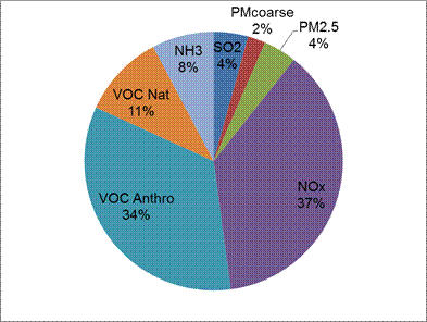
Figure 5.1 Emission inventory of air pollutants for (a) the Canadian Lower Fraser Valley for the year 2010 and (b) the Puget Sound airshed for the year 2011.
(a)
(b)

Notes: PM coarse is the size fraction of PM between 2.5 and 10 μm.
Emissions from road dust are not included for PM coarse and PM2.5 but are quantified below.
“Nat” and “Anthro” are Natural and Anthropogenic emissions, respectively.
(a) In the Canadian Lower Fraser Valley, total emissions of these contaminants were 140 kilotonnes in 2010 (Metro Vancouver, 2013).Road dust emissions were 5 kilotonnes in 2010 (Metro Vancouver, 2013).
(b) In the Puget Sound airshed, total emissions of these contaminants were 511 kilotonnes in 2011 (WA DOE, 2014). Road dust emissions were 15 kilotonnes in 2011 (WA DOE, 2014).
Description of Figure 5.1
Figure 5.1 concsists of two pie charts. In the first the emission inventory of air pollutants for the Canadian Lower Fraser Valley is shown. The pollutants and their percentages are as follows. SO2: 3%, PM Coarse: 5%, PM2.5: 4%, NOx: 33%, VOC anthropogenic: 38%, VOC natural: 9%, NH3: 8%. In the Lower Fraser Valley, total emissions of these contaminants were 156 kilotonnes in 2005. (Metro Vancouver, 2007)
In the second the emission inventory of air pollutants for the Puget Sound airshed is shown. The pollutants and their percentages are as follows. SO2: 5%, PM Coarse: 5%, PM2.5: 5%, NOx: 29%, VOC anthropogenic: 26%, VOC natural: 31%, NH3: 3%. In the Puget Sound airshed, total emissions of these contaminants were 607 kilotonnes in 2005. (WA DOE, 2007).
The figure has the following notes
- PM coarse is the size fraction of PM between 2.5 and 10 μm.
- PM coarse and PM2.5 include emissions from road dust.
| Pollutant | Source | Estimated Confidence Of Category in Overall Inventory | |
|---|---|---|---|
| Canada | USA | ||
| SO2 |
Electric Utility
|
H
|
H
|
|
Ind. / Comm. Fuel Comb.
|
M
|
M
|
|
|
Other Fuel Comb.
|
M
|
M
|
|
|
Transportation
|
M
|
M
|
|
|
Industrial Processes
|
M
|
M
|
|
|
Other Anthropogenic (Non Comb.)
|
L
|
L
|
|
|
Natural
|
L
|
L
|
|
| NOx |
Electric Utility
|
M-H
|
H
|
|
Ind. / Comm. Fuel Comb.
|
M
|
M
|
|
|
Other Fuel Comb.
|
M
|
M
|
|
|
Transportation
|
H
|
H
|
|
|
Industrial Processes
|
M
|
M
|
|
|
Other Anthropogenic (Non Comb.)
|
L
|
L
|
|
|
Natural
|
M
|
M
|
|
| VOCsa |
Electric Utility
|
M-H
|
M-H
|
|
Ind. / Comm. Fuel Comb.
|
M
|
M
|
|
|
Other Fuel Comb.
|
L
|
L
|
|
|
Transportation
|
M
|
H
|
|
|
Industrial Processes
|
M
|
M
|
|
|
Other Anthropogenic (Non Comb.)
|
L
|
L
|
|
|
Natural
|
M
|
M
|
|
| NH3 |
Electric Utility
|
M
|
M
|
|
Ind. / Comm. Fuel Comb.
|
L
|
L
|
|
|
Other Fuel Comb.
|
L
|
L
|
|
|
Transportation
|
M
|
M
|
|
|
Industrial Processes
|
L
|
L
|
|
|
Other Anthropogenic (Non Comb.)
|
L-M
|
L
|
|
|
Natural
|
L
|
L
|
|
| PM10b |
Electric Utility
|
M
|
M
|
|
Ind. / Comm. Fuel Comb.
|
M
|
M
|
|
|
Other Fuel Comb.
|
L
|
L
|
|
|
Transportation
|
M
|
M
|
|
|
Industrial Processes
|
M
|
M
|
|
|
Other Anthropogenic (Non Comb.)
|
L
|
L
|
|
|
Natural
|
L
|
L
|
|
| PM2.5c |
Electric Utility
|
M/L
|
M/L
|
|
Ind. / Comm. Fuel Comb
|
M/L
|
M/L
|
|
|
Other Fuel Comb.
|
L
|
L
|
|
|
Transportation
|
L
|
M
|
|
|
Industrial Processes
|
L
|
L
|
|
|
Other Anthropogenic (Non Comb.)
|
L
|
L
|
|
|
Natural
|
L
|
L
|
|
Notes:
a For total VOCs, speciation estimates rated at a low confidence level
b For total PM, composition profiles rated as low to medium confidence levels
c EPA’s Non-Road Model
Description of Table 5.1
Table 5.1 summarizes the level of confidence in the emissions estimates for a range of pollutants and their various sources in both Canada and the US.
The first row of the table contains the headers “Pollutant”, “Source”, and “Estimated Confidence of Category in Overall Inventory”. The last header is further divided into two subcategories; Canada and the USA. The first column shows the different pollutants which are SO2, NOx, VOCs (note that for total VOCs, speciation estimates rated at a low confidence level), NH3, PM10 (note that For total PM, composition profiles rated as low to medium confidence levels), and PM2.5 (EPA’s Non-Road Model). The third column gives the possible sources for each pollutant listed in the first column. In all cases these are as follows:
- Electric Utility
- Industrial / Commercial Fuel Combustion
- Other Fuel Combustion
- Transportation
- Industrial Processes
- Other Anthropogenic (Non Combustion)
- Natural
The fourth and fifth columns give the estimated confidence (Low (L), Medium (M), or High(H)) of the category in the overall inventory for Canada and the USA respectively.
5.2.1 Uncertainties in Emission Inventories
Although emission inventory methodologies are well accepted and documented, considerable uncertainty remains. In Table 5.1, the criteria air contaminants are listed next to their source categories. An estimate of the level of confidence, rated as high (H), medium (M), or low (L) is included, based on studies referenced in the NARSTO PMAssessment (NARSTO, 2004). Additional approaches that can be used to reconcile emission inventories with measurements of species concentrations observed in the atmosphere need to be developed (NARTSO, 2004).
5.2.2 Caveat on Uncertainties in Emission Inventories
Since the publication of the NARSTO PM Assessment report (2004), it is likely that the confidence in emissions from several sources have improved as a result of better assimilation of available data. For instance, confidence in emissions from the transportation sector have likely improved, as a result of spatial and temporal enhancement in the monitoring network. Confidence in emission estimates from electric utilities has likely improved due to closures of coal power plants in the area. In addition, improvements in estimates from industrial processes are likely to have occurred due to improvements in temporal profiles of emissions.
5.2.3 Contaminant Emissions in the Georgia Basin
Total emissions of selected criteria air contaminants (NOx, SOx, VOCs, NH3, and PM) were 140 kilotonnes (including 14 kilotonnes of VOCs from vegetation) in 2010 for the Canadian Lower Fraser Valley (Metro Vancouver, 2013). VOCs and NOx comprised the highest contaminant emissions. The contribution from anthropogenic VOCs and NOx was 71% of total contaminants.
Caveat on Biogenic Emissions
The estimates of VOCs from vegetation in the Canadian Lower Fraser Valley were based on an emissions inventory for the year 2000, prorated based on vegetation land cover data from 2006 and 2001(Metro Vancouver, 2014; GVRD, 2003). While estimates of VOCemissions from vegetation are an important “background” source to consider in air quality management, they are natural sources and are not candidates for emission control. If natural VOCs are excluded from the total emissions of CACs (excluding CO emissions), the combined contribution from anthropogenic VOCs and NOx is 80% in the Canadian Lower Fraser Valley.
5.2.4 Contaminant Emissions in the Puget Sound
Total emissions of the criteria contaminants (NOx, SOx, VOCs, NH3, and PM) were 511 kilotonnes in 2011 for the Puget Sound, including 150 kilotonnes from vegetation. The emissions estimates for vegetation were based on EPA’s 2011 National Emission Inventory version 1 (WA DOE, 2014; U.S. EPA, 2013). VOCs and NOx comprise the highest contaminant emissions. The combined contribution from natural and anthropogenic VOCsand NOx is 84%. If natural VOCs are excluded from the total emissions, the combined contribution from anthropogenic VOCsand NOx is 78%.
Caveat on Comparing Emissions from the Georgia Basin and the Puget Sound
The reader is strongly advised not to draw conclusions based on comparing the separate inventories from the Georgia Basin (Canadian Lower Fraser Valley) and the Puget Sound. Apparent differences in emissions may instead reflect differences in estimation models, methodologies, emission rates, source categories, and data availability (WA DOE, 2014; Metro Vancouver, 2013).
For the same reasons, inventories in the 2004 Characterization of the Georgia Basin/Puget Sound Airshed report are not compared to results presented here. However, a backcast analysis for the Canadian Lower Fraser Valley is presented later in this chapter which compares emission changes from 1990 to 2010.
5.2.5 Sources of Emissions by Sector
The emissions in an airshed can be reduced by controlling their sources. Some emission control programs target sources and sectors that emit multiple pollutants. A recent example is the ratification of an international agreement under the International Maritime Organization to establish an Emissions Control Area targeting marine emissions of SO2, NOx and PM within 200 nautical miles off the North American coast of the Pacific and Atlantic Oceans, including the coast of the Georgia Basin/Puget Sound airshed (IMO, 2010). Figure 5.2 and Figure 5.3 show the sectors with the highest total annual emissions of smog-forming pollutants by mass (NOx, VOC, PM2.5, SOx and NH3).
Figure 5.2 implies that light duty vehicles (18%), chemical product use (16%) and non-road sources (12%) released significant levels of smog-forming emissions in the Canadian Lower Fraser Valley in 2010. The transportation sector, including light and heavy-duty vehicles and marine sources, accounts for one third of total emissions. Emission control scenarios for vehicles, industrial point sources, marine and agricultural sources are discussed in Chapter 10, “Regional Air Quality Modelling”.
For the year 2011, the Puget Sound airshed emitted approximately 488 kilotonnes of smog-forming emissions. Natural emissions, primarily composed of VOCs from vegetation, were the largest source (31%) in the airshed. Transportation, including light and heavy-duty vehicles and marine sources, accounted for over one third of total emissions. Industrial point sources, non-road mobile equipment and chemical product usage were also important contributors. Residential woodstoves and fireplaces, used for heating by many Puget Sound residents, contributed 5% of the total emissions.
Figure 5.2 2010 Smog-forming emissions by sector in the Canadian Lower Fraser Valley.
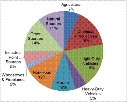
Notes: Based on percent by mass of NOx, VOCs, PM2.5, SOx and NH3. Total emissions of 137 kilotonnes in 2010 (Metro Vancouver, 2013).
Description of Figure 5.2
Figure 5.2 is a pie chart of Smog-forming emissions by sector in the Canadian Lower Fraser Valley. The sectors and their percentage of total smog-forming emissions are as follows. Agricultural: 7% , solvent evaporation: 14%, light-duty vehicles: 20%, heavy-duty vehicles: 4%, marine: 8%, non-road: 14%, woodstoves and fireplaces: 1%, industrial point sources: 8%, other sources: 14%, natural sources: 10%.
The figure has the following notes:
- Based on percent by mass of NOx, VOC, PM2.5, SOx and NH3
- Total emissions of 148 kilotonnes in 2005 (Metro Vancouver, 2010)
Figure 5.3 2011 Smog-forming emissions by sector in the Puget Sound.
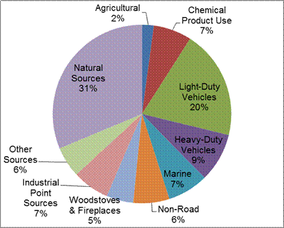
Notes: Based on percent by mass of NOx, VOCs, PM2.5, SOx and NH3. Total emissions of 488 kilotonnes in 2011 (WA DOE, 2014).
Description of Figure 5.3
Figure 5.3 is a pie chart of Smog-forming emissions by sector in the Puget Sound. The sectors and their percentage of total smog-forming emissions are as follows. Agricultural: 3% , solvent evaporation: 3%, light-duty vehicles: 19%, heavy-duty vehicles: 9%, marine: 8%, non-road: 8%, woodstoves and fireplaces: 6%, industrial point sources: 10%, other sources: 2%, natural sources: 32%.
The figure has the following notes:
- Based on percent by mass of NOx, VOC, PM2.5, SOx and NH3
- Total emissions of 590 kilotonnes in 2005 (WA DOE, 2007)
5.2.6 Sources of Emissions by Contaminant
Different contaminants have different health and environmental impacts. When a particular contaminant is of concern, such as PM2.5, it is useful to know the major sources of its direct emissions. Figure 5.4 and Figure 5.5show the major emission sources by sector and contaminant in the Canadian Lower Fraser Valley and the Puget Sound, respectively. Table 5.2 identifies the key emission sources for each pollutant in both the Georgia Basin and the Puget Sound.
Figure 5.4 depicts some of the complexity involved in controlling emission sources to improve air quality. VOCs, NOx, and PM2.5 each have multiple important emissions sources emerging from a variety of industrial and domestic activities.
For sulphur dioxide, marine sources are the single largest contributing sector in the Canadian Lower Fraser Valley (79%). Recent studies of the impact of marine sources across Canada and the United States resulted in the adoption of an Emission Control Area by the International Maritime Organization in 2010 (IMO, 2010). For ammonia, agriculture remains the dominant source (73% in the Canadian Lower Fraser Valley and 76% in the Puget Sound). Emissions estimation and control of agricultural ammonia remains a challenge due to the variability and geographic extent of these sources, but a recent Environment Canada report attempted to address these issues (Environment Canada, 2010). Both the marine and agricultural emissions investigations are discussed in Chapter 10.
Figure 5.4 2010 contaminant emissions by sector in the Canadian Lower Fraser Valley (Metro Vancouver, 2013).
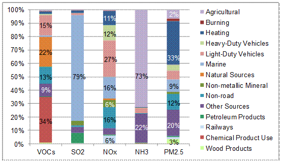
Description of Figure 5.4
Figure 5.4 is a stacked column chart showing percentage of emissions by sector for VOCs, SO2, NOx, NH3, and PM2.5. The sectors are agriculture, burning, heating, heavy-duty vehicles, light-duty vehicles, marine, natural sources, non-metallic mineral, non-road, other sources, petroleum products, railways, solvent evaporation, and wood products.
For VOCs 27% of emissions are from burning, 9% are from other sources, 14% are from non-road, 19% are from natural sources, and 21% are from light-duty vehicles. For SO2 69% of emissions are from marine sources. For NOx 7% of emissions are from railways, 19% are from non-road sources, 7% are from non-metallic mineral sources, 14% are from marine sources, 26% are from light-duty vehicles, 9% are from heavy-duty vehicles, and 11% are from heating. For NH3 20% of emissions are from other sources, and 66% are from agricultural sources. For PM2.5 5% of emissions are from wood products, 34% are from other sources, 12% are from non-road sources, 7% are from marine sources, 16% are from heating, and 14% are from burning.
The figure has a note that 11% of total PM2.5 emissions are from road dust, captured in the “Other” category.
Figure 5.5 2011 contaminant emissions by sector in Puget Sound (WA DOE, 2014).
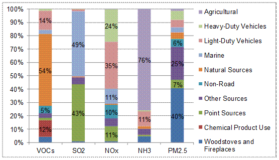
Description of Figure 5.5
Figure 5.5 is a stacked column chart showing percentage of emissions by sector for VOCs, SO2, NOx, NH3, and PM2.5. The sectors are agriculture, heavy-duty vehicles, light-duty vehicles, marine, natural sources, non-road, other area sources, point sources, solvent evaporation, and woodstoves and fireplaces.
For VOCs 8% of emissions are from woodstoves and fireplaces, 6% are from solvent evaporation, 6% are from non-road sources, 54% are from natural sources, and 17% are from light-duty vehicles. For SO252% of emissions are from point sources, 7% are from non-road sources, and 32% are from marine sources. For NOx 18% of emissions are from point sources, 14% are from non-road sources, 12% are from marine sources, 27% are from light-duty vehicles, and 26% are from heavy-duty vehicles. For NH3 16% of emission s are from light-duty vehicles, and 80% are from agricultural sources. For PM2.5 44% of emissions are from woodstoves and fireplaces, 13% are from point sources, and 9% are from non-road sources.
The figure has the following notes.
- 8% of total PM2.5 emissions are from residential trash burning, captured in the “Other Area Sources” category.
- Road dust is estimated to be a minimal component of PM2.5 emissions in the Puget Sound, but is an important component of PM10, which is not shown in this figure.
| Dominant Emission Sectors | ||
|---|---|---|
| Criteria Air Contaminant | Puget Sound - 2011 | Georgia Basin (CLFV) - 2010 |
| VOCs |
|
|
| SO2 |
|
|
| NOx |
|
|
| NH3 |
|
|
| PM10* |
|
|
| PM2.5* |
|
|
* Road dust emissions are not included in the table above. In 2011, road dust emissions contributed 21% and 9% of total PM10 and PM2.5 emissions, respectively, in the Puget Sound (WA DOE, 2014). In the CLFV, the contribution from road dust emissions was 34% and 16% of total PM10 and PM2.5 emissions, respectively, in 2010 (Metro Vancouver, 2013).
Description of Table 5.2
Table 5.2 presents the dominant emissions sectors for six pollutants in the Georgia Basin and Puget Sound airsheds in 2005.
The first row of the table contains the title “Dominant Emission Sectors - 2005”
The second row of the table contains the headers “Common Air Contaminant”, “Puget Sound”, and “Georgia Basin (CLFV)”. The first column shows the different air contaminants being considered. These are:
- VOCs
- SO2
- NOx
- NH3
- PM10
- PM2.5
The third and fourth columns list the dominant emissions sectors for each contaminant in Puget Sound and the Georgia Basin respectively.
5.3 Emission Forecasts
Emissions forecasts are based on projected changes in activity (growth or decline) combined with changes in emission rates and reduction measures. Changes in emissions can be driven by technological, regulatory, social or economic developments. Therefore, it is very important to understand which of the various control strategies and new sources have been considered in the estimation of the forecast emission levels. The assumptions used to develop the forecast emissions for the Georgia Basin/Puget Sound airshed can be found in Metro Vancouver (2013) and WRAP (2007).
The emissions inventory forecast for 2018 developed by WRAP was based on the 2002 inventory (WRAP, 2007). Emissions estimates for the Canadian Lower Fraser Valley portion of the Georgia Basin were forecast from 2010 to 2030 (Metro Vancouver, 2013).
5.3.1 Emissions in the Puget Sound
Some of the known control programs that are included in the WRAP 2018 scenario include (T. Moore, pers. comm.):
- Smoke management programs
- New permits and state/EPA consent agreements since 2002
- Ozone and PM10 State Implementation Plans (SIPs) in place within the WRAP region
- State oil and gas emission control programs
- Mobile sources: Heavy Duty Diesel (2007) Engine Standard; Tier 2 Tailpipe; Large Spark Ignition and Recreational Vehicle Rule; Non-road Diesel Rule
- Combustion Turbine and Industrial Boiler/Process Heater/RICE MACT
- VOC 2, 4, 7 and 10-year MACT Standard
- Presumptive SO2 Best Available Retrofit Technologies
The emissions of smog-forming pollutants for the entire Puget Sound airshed are forecast to decrease by 21% from 2002 to 2018. Figure 5.6 shows how much the total emissions will change in every county. Figure 5.7 shows how the overall decrease of 21% varies by contaminant. Generally, emissions of NH3 and PM2.5 are expected to rise throughout Puget Sound, while emissions of the remaining contaminants will decrease.
Figure 5.6 Comparison of 2002 smog-forming emissions and 2018 forecast for Puget Sound counties.
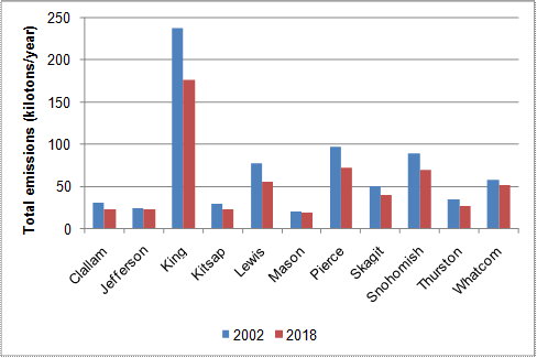
Notes: Based on total mass of NOx, VOC, PM2.5, SOx and NH3 (WRAP, 2007)
Description of Figure 5.6
Figure 5.6 is a bar chart showing a comparison of 2002 smog-forming emissions and 2018 forecast smog-forming emissions for Clallam, Jefferson, King, Kitsap, Lewis, Mason, Pierce, Skagit, Snohomish, Thurston, and Whatcom counties. The values plotted are total emissions in kilotons/year. The values are based on total mass of NOx, VOC, PM2.5, SOx and NH3 (WRAP, 2007). The emissions values are as follows.
- For Clallam the 2002 value is approximately 30 kilotons/year and the 2018 values is approximately 25 kilotons/year.
- For Jefferson the 2002 value is approximately 25 kilotons/year and the 2018 values is approximately 25 kilotons/year.
- For King the 2002 value is approximately 240 kilotons/year and the 2018 values is approximately 175 kilotons/year.
- For Kitsap the 2002 value is approximately 25 kilotons/year and the 2018 values is approximately 20 kilotons/year.
- For Lewis the 2002 value is approximately 75 kilotons/year and the 2018 values is approximately 55 kilotons/year.
- For Masin the 2002 value is approximately 20 kilotons/year and the 2018 values is approximately 20 kilotons/year.
- For Pierce the 2002 value is approximately 95 kilotons/year and the 2018 values is approximately 75 kilotons/year.
- For Skagit the 2002 value is approximately 50 kilotons/year and the 2018 values is approximately 40 kilotons/year.
- For Snohomish the 2002 value is approximately 85 kilotons/year and the 2018 values is approximately 75 kilotons/year.
- For Thurston the 2002 value is approximately 30 kilotons/year and the 2018 values is approximately 25 kilotons/year.
- For Whatcom the 2002 value is approximately 55 kilotons/year and the 2018 values is approximately 50 kilotons/year.
Figure 5.7. Percent change in smog-forming emissions from 2002 to 2018 by contaminant
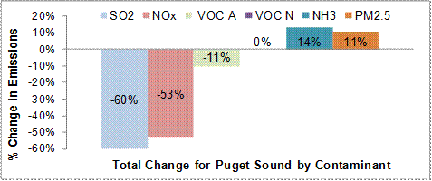
Notes: "N" and "A" are Natural and Anthropogenic emissions (WRAP, 2007)
Description of Figure 5.7
Figure 5.7 is a bar chart showing the percent change in smog-forming emissions in Puget Sound from 2002 to 2018 broken down by contaminant. For SO2 the percent change is -60%, for NOxthe percent change is -53%, for anthropogenic VOCs the percent change is -11%, for natural VOCs the percent change is 0%, for NH3 the percent change is 14%, and for PM2.5 the percent change is 11%.
Emissions of NOx are estimated to decrease more than those of VOCs, which has consequences for ozone formation. Similarly, emissions of NOx and SO2 will decrease more than those of NH3, which can impact the formation and composition of secondary particulate matter (PM2.5).
Natural VOCs are primarily emitted by forest fires and by the biological processes of plants and trees. Natural emissions appear unchanged in Figure 5.7 because emissions from vegetation were held constant from the year 2002, and forest fire emissions were held constant, based on the average of emissions from the years 2000 to 2004 (WRAP, 2007).
5.3.2 Emissions in the Georgia Basin
The 2010 emissions forecast in the Canadian Lower Fraser Valley (Metro Vancouver, 2013) incorporated all committed federal, provincial and regional activities and policy measures, as well as new emission sources. Some of the forecasted policy measures and new sources quantified in the forecast include:
- Metro Vancouver’s Boilers and Heaters Regulation;
- British Columbia’s AirCare Inspection and Maintenance program (until 2014, after which emissions testing ends for light duty vehicles;
- International Maritime Organization (IMO) Emission Control Area (ECA) and IMO Annex VI marine regulations;
- Marine vessel activity related to projected growth in shipping
- New and Expanded Coal Terminals
Other potential policy measures and new sources which were noted but not quantified for reasons such as uncertain implementation status, lack of data and low impact are:
- BC Building Code Energy Requirements
- BC Open Burning Smoke Control Regulation
- New district energy systems
- Federal Based Level Industrial Emission Requirements (BLIERS)
- Heavy Duty Vehicles Retrofit Requirement (Provincial)
For further details on the policy measures and sources included in the forecast, refer to Metro Vancouver (2013).
Figure 5.8 shows trends in Canadian Lower Fraser Valley emissions by pollutant since 1990. Most emissions have declined and are expected to continue to do so, with the exception of VOCs, ammonia and PM10, which are expected to increase after 2015. Figure 5.9 shows that in 2010, light-duty vehicles were the largest source of smog-forming pollutants; however, due to the improved vehicle emission standards, contributions from light-duty vehicles are expected to decrease until 2020. By 2030, chemical products usage is projected to be the largest source of smog-forming pollutants in the CLFV. It should be noted that the new marine emission control regulations significantly affect the emissions projections for the international Lower Fraser Valley. As shown in Figure 5.10, without these regulations, marine emissions in the international Lower Fraser Valley in 2030 would be similar to those in 2010. Please refer to Metro Vancouver (2010) for further details.
Figure 5.8. Forecast and backcast emissions compared to 2005 base year for the Canadian Portion of the WISE (Metro Vancouver, 2010)
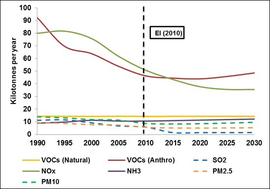
Notes: "N" and "A" are Natural and Anthropogenic emissions (WRAP, 2007)
Description of Figure 5.8
Figure 5.8 is a plot of the emissions of NOx, NH3, PM10, PM2.5, VOCs (natural and anthropogenic), and SO2 in kilotonnes/year from 1990 through 2030. The values are forecast and backcast based on 2005.
For Anthropogenic VOCs the 2005 emissions were just over 60 kilotons/year. The backcast shows a steady decline from emissions of 100 kilotons/year in 1990. The forecast predicts a continued decline to approximately 50 kilotons/year in 2010 followed by a slow but steady increase to between 55 and 60 kilotons/year in 2030.
For NOx the 2005 emissions were just over 50 kilotons/year. The backcast shows a steady decline from emissions of 85 kilotons/year in 1990. The forecast predicts a continued decline to approximately 40 kilotons/year in 2020 where levels will remain through 2030.
For PM10 the 2005 emissions were approximately 15 kilotons/year. The backcast shows this to be very slight decline of no more than 1 kiloton/year from 1990 and the forecast predicts a very slight increase of no more than 2 kilotons/year by 2030.
For natural VOCsthe 2005 emissions were approximately 15 kilotons/year and no change was seen in the backcast or forecast.
For NH3 the 2005 emissions were just below 15 kilotons/year. This was an increase from approximately 10 kilotons/year in 1990 and emissions are predicted to rise to 15 kilotons/year by 2030.
For SO2 the 2005 emissions were approximately 5 kilotons/year. This was a decrease from approximately 10 kilotons/year in 1990 and the emissions of SO2 are expected to rise slightly to between 5 and 10 kilotons/year by 2030.
For PM2.5 the 2005 emissions were approximately 5 kilotons/year which was a slight decline of no more than 1 kiloton/year from 1990. No increase is expected through 2030.
Figure 5.9. Forecast and backcast of sector-specific smog-forming pollutant emissions in the WISE based on 2005 base year (Metro Vancouver, 2010)
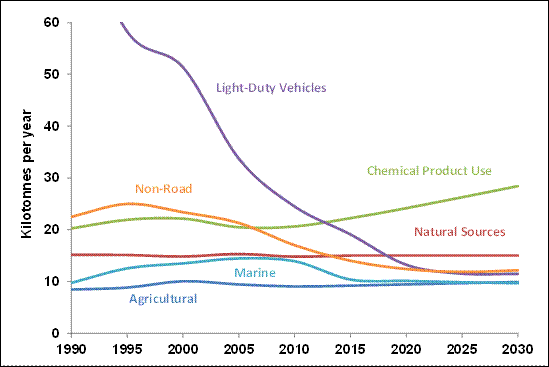
Description of Figure 5.9
Figure 5.9 is a plot of the emissions by six different sectors in kilotonnes/year from 1990 through 2030. The values are forecast and backcast based on 2005.
Emissions by light-duty vehicles fell from 60 kilotons/year to 30 kilotons/year between 1997 and 2005. This decrease is predicted to level off at approximately 15 kilotons/year by 2020.
For natural sources the 2005 emissions were just above 35 kilotons/year. There was a very slight decline of no more than 2 kilotons/year from 1990 to 2005, but emissions are expected to remain at 2005 levels through 2030.
For non-road sources there was a slight increase from just above 25 kilotons/year in 1990 to approximately 30 kilotons/year in 1995. This then fell to approximately 20 kilotons/year in 2005 and is expected to decline to approximately 15 kilotons/year by 2020 with steady emission levels thereafter.
For solvent evaporation there was a slight increase from just above 20 kilotons/year in 1990 to just below 25 kilotons/year in 2000. This then fell back to approximately 20 kilotons/year in 2005 and is expected to fall to slightly below 20 kilotons/year by 2010. After 2010 a steady increase to just over 25 kilotons/year is expected.
For marine sources there has been a steady increase from just over 10 kilotons/year in 1990 to just below 15 kilotons/year in 2005. A further increase to just over 20 kilotons/year is expected by 2030.
Figure 5.10. Forecast of smog-forming pollutants in the WISE based on implementation of IMO Annex VI (April 2008 MEPC recommendations) (Metro Vancouver, 2010)
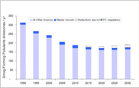
Description of Figure 5.10
Figure 5.10 is a stacked bar chart of emissions of smog-forming pollutants in kilotonnes/year for every fifth year from 1990 to 2030. Emissions from marine vessels, from all other sources, and the predicted reductions in marine emissions due to MEPC regulations are shown.
In 1990 emissions from marine vessels were approximately 10 kilotonnes/year while emissions from all other sources were approximately 300 kilotonnes/year. Emissions from all other sources fell steadily from 1990 to 2010 where they reached a level of approximately 175 kilotonnes/year. In that same time emissions from marine sources rose steadily to approximately 20 kilotonnes/year. From 2015 to 2030 emissions from all other sources are expected to remain steady while emissions from marine sources without the MEPC regulations would continue to increase to approximately 30 kilotonnes/year. With the MEPC regulations in place marine emissions are expected to decline in 2015 to approximately 10 kilotonnes/year and remain at that level through 2030.
Table 5.3 illustrates the predicted changes in emissions for the Canadian Lower Fraser Valley in 2030 in comparison to 2010. Emissions of NOx and SO2 are expected to decline, whereas anthropogenic VOCs, ammonia, and PM10 will rise. An analysis of the contaminant sources and assumptions included in the estimates can help explain the changes in emissions.
| Contaminant | Percent Change from 2010 to 2030 |
|---|---|
| NOx |
-30%
|
| SO2 |
-74%
|
| VOC (anthropogenic) |
+5%
|
| NH3 |
+15%
|
| PM10 |
+11%
|
| PM2.5 |
-6%
|
Description of Table 5.3
Table 5.3 presents the predicted change in emissions for six different air contaminants in Puget Sound (2002-2018) and the Canadian Lower Fraser Valley (2005-2020).
The first row of the table contains the headers “Contaminant” and “Predicted Change in Emissions”. This last header is further subdivided into “Puget Sound 2002-2018”, and “CWISE2005-2020”. The first column shows the different air contaminants being considered. These are:
- NOx
- SO2
- VOC(anthropogenic)
- NH3
- PM10(includes road dust)
- PM2.5(includes road dust)
The third and fourth columns show the predicted percent change in emissions for each contaminant in Puget Sound and the Canadian Lower Fraser Valley respectively.
The large projected decrease in SO2 emissions in the CWISE is due to the implementation of the North American Emission Control Area (ECA), of which phase 1 took effect in August 2012 and phase two will take in effect in January 2015. Consequently total SO2 emissions are expected to decline by 74% over the period 2010-2030 (Metro Vancouver, 2013), with most of the decline occurring in the first five years after the implementation of the new marine regulations. The emission forecast takes into account a number of permit changes, activity levels and regulation implementation. The main contributors of SO2 emissions in the future include primary metal industries in Whatcom County and industrial sources, such as petroleum refining and marine vessels (Metro Vancouver, 2013).
Emissions of NOxoriginate mainly from mobile sources, namely cars and trucks (on-road), non-road equipment and marine vessels. Moderate decreases in NOx emissions are expected for the CWISE until around 2025, after which the emissions are projected to remain relatively constant. In the future, marine vessels are projected to become one of the dominant sources of NOx due to projected growth in shipping; however, growth in NO2 will be mitigated over time with the 2016 implementation of IMO Annex VI Tier III marine engine standards).
Anthropogenic volatile organic compound (VOC) emissions are projected to decrease until 2015 in the CWISE as a result of stricter vehicle emissions standards, vehicle emission inspection programs, as well as controls to decrease VOC emissions from architectural coatings and commercial and consumer products. VOC emissions are projected to rise again after 2020 due to an increase in emissions from chemical product use and are expected to surpass the 2010 levels by 2030 (Metro Vancouver, 2013).
The vast majority of ammonia emissions are due to agricultural practices in both airsheds. In the CLFV, ammonia emissions are expected to rise over the next decade due to growth in the agricultural sector, increase in light-duty vehicle use, and increased loading on wastewater treatment facilities. Ammonia emissions from on-road vehicles also play a role in the CLFV, although these are much less than those from the agricultural sector.
PM10 emissions in the CLFV are expected to increase by 10% in 2030 over the period 2010 to 2030, reflecting projected growth largely in the construction sector.
5.4 Emission Changes and Ambient Air Quality
As emissions are forecast to change over next few decades, it is important to understand their impact on ambient concentrations of air pollutants in order to lay the foundation for discussing approaches to air quality management and to develop potential pollution control measures. This can be achieved through computer modelling which can estimate air quality concentrations, based on emission quantities. A more in-depth discussion on the tools and models used to evaluate the air quality consequences of proposed emission changes in the Georgia Basin/Puget Sound airshed can be found in Chapter 10: Regional Air Quality Modelling.
Ozone, fine particulate matter and other pollutants are related through a complex interaction of common emissions and precursors, physical and chemical processes and meteorology. This interaction is captured in Table 5.4, where the reduction in emissions of criteria air contaminants is related to the impacts on ozone and fine particulate concentrations, as well as to PM composition and acid deposition. Table 5.4 contains important information beyond the obvious relationships between increases and decreases in emissions and pollutants or associated atmospheric issues.
Reducing emissions of NOx has a varied impact on both ozone and PM concentrations. Near and downwind of some urban centres where VOC concentrations are limited, NOx emission reductions can cause ozone concentrations to increase. However, decreased NOx emissions provide larger ozone reductions farther downwind. The presence of lower NOx concentrations influences the composition of PM, where the oxidized nitrogen might be replaced by sulphate. The organic compound fraction of PM may increase or decrease, depending on the effect of NOx on oxidant levels. Therefore, lowering NOx emissions does not guarantee that the concentrations of ozone or PM will decrease; in fact, the concentrations could easily increase in some areas under specific atmospheric conditions.
The last three entries in Table 5.4indicate that decreases in black carbon, primary organic compounds and other primary PM can be associated with increases in ozone, but decreases in PM2.5 concentrations.
Table 5.4 Emission reductions and associated changes in ozone, PM, and acid deposition (adapted from NARSTO, 2004).
| Reduction in Pollution Emissions | Change in Associated Pollutant or Atmospheric Issue | |||||
| Ozone | PM Composition | PM2.5(j) | Acid Deposition | |||
| Sulphate | Nitrate | Organic Compounds | ||||
| SO2 | decrease | increase(d) | decrease | decrease | ||
| NOX | decrease; possible small increase | possible small increase/ decrease(b) | decrease(e) | possible small increase/ decrease(g) | decrease; possible small increase | decrease; possible small increase |
| VOC | decrease | possible small increase/ decrease | decrease; possible small increase(f) | decrease(h) | decrease; possible small increase | decrease; possible small increase |
| NH3 | possible small decrease(c) | decrease | decrease | increase(k) | ||
| Black Carbon | possible small Increase(a) | possible small decrease(i) | decrease | |||
| Primary Organic Compounds | possible small Increase(a) | decrease | decrease | |||
| Other Primary PM | possible small Increase(a) | decrease | increase(k) | |||
Blue arrows indicate decreases and red arrows indicate increases. The size of the arrow relates to the amount of change. A blank entry suggests a negligible response.Note:
a In and downwind of some urban areas that are VOC limited.
b Effect on daytime ozone due to increase in solar flux and decrease in radical scavenging; effect on night time ozone unknown.
c Due to effect of NOx on oxidant levels (OH, H2O2 and ozone); e.g., see SAMI (Southern Appalachian Mountains Initiative) modeling results.
d Due to effect of NH3 on cloud/ fog pH.
e Decrease in sulfate may make more NH3available for reaction with HNO3 to form NH4NO3, more important when NH4NO3 is NH3 limited.
f Decrease except special cases (e.g., SJV); decrease in NOx may lead to increase in ozone with associated increase in HNO3 formation.
g Increase due to less organic nitrate formation and more OH available for reaction with NO2; decrease due to decrease in oxidant levels.
h Related to effect of NOx on oxidant levels (OH, ozone, and NO3-).
i Decrease of secondary component; magnitude depends on OC fraction that is secondary anthropogenic.
j Reduction of OC adsorbed or emitted with black carbon.
k Refers to net acidity atmospheric deposition, not to acidification potential to ecosystem.
Description of Table 5.4
Table 5.4 presents the predicted changes in three atmospheric pollutants or issues (ozone, PM, and acid deposition) that are associated with reductions in seven different primary emissions.
The first column of the table contains the header “Reduction in Pollution Emissions” and shows the different primary air contaminants for which reductions will result in changes in PM, ozone, or acid deposition. These are:
- SO2
- NOx
- VOC
- NH3
- Black carbon
- Primary organic compounds
- Other primary PM
The table has six additional columns which share the title “Change in associated pollutant or atmospheric issue”. These columns have the headers “Ozone”; “PM Composition”, which is further subdivided into columns with headers “Sulphate”, “Nitrate”, and “Organic Compounds”; “PM2.5”, and “Acid deposition”. Under each of these heading there are arrows indicating the type and magnitude of change associated with a reduction of the emissions listed in column 1. Blue arrows indicate decreases and red arrows indicate increases. The size of the arrow relates to the amount of change. A blank entry suggests a negligible response.
Reductions in SO2 emissions result in a large decrease in sulfate PMcomposition, a slight increase in nitrate PM composition (due to the effect of NH3 on cloud/ fog pH), and a large decrease in PM2.5 and acid deposition. Responses of the other pollutants or issues are negligible.
Reductions in NOxemissions result in both a large decrease and a slight increase in ozone and both a slight decrease and a slight increase in sulfate PM composition (there is a note that the effect on daytime ozone is due to increase in solar flux and decrease in radical scavenging; the effect on night time ozone is unknown). Reductions in NOx emissions also result in a large decrease in nitrate PMcomposition (there is a note that the decrease in sulfate may make more NH3 available for reaction with HNO3to form NH4NO3, more important when NH4NO3 is NH3 limited.), both a slight decrease and a slight increase in organic compounds PM composition (there is a note that the increase is due to less organic nitrate formation and more OH available for reaction with NO2; decrease due to decrease in oxidant levels), both a large decrease and a slight increase in PM2.5, and both a large decrease and a slight increase in acid deposition.
Reductions in VOC emissions result in a large decrease in ozone, both a slight decrease and a slight increase in sulfate PM composition, and both a large decrease and a slight increase in nitrate PM composition (there is a note that there is a decrease except special cases (e.g., SJV) and the decrease in NOx may lead to increase in ozone with associated increase in HNO3 formation). Reductions in VOC emissions also result in a large decrease in organic compounds PM composition (related to the effect of NOx on oxidant levels (OH, ozone, and NO3-)), both a large decrease and a slight increase in PM2.5, and both a slight decrease and a slight increase in acid deposition.
Reductions in NH3emissions result in a large decrease in sulfate PM composition (due to the effect of NOx on oxidant levels (OH, H2O2 and ozone); e.g., see SAMI (Southern Appalachian Mountains Initiative) modeling results). Reductions in NH3 emissions also result in a large decrease in nitrate PM composition, a large decrease in PM2.5, and a large increase in acid deposition (this refers to net acidity atmospheric deposition, not to acidification potential to ecosystem). Responses of the other pollutants or issues are negligible.
Reductions in black carbon emissions result in a slight increase in ozone (in and downwind of some urban areas that are VOC limited), a slight decrease in organic compounds PMcomposition (this is decrease of secondary component; magnitude depends on OC fraction that is secondary anthropogenic), and a large decrease in PM2.5.
Reductions in primary organic compounds emissions result in a slight increase in ozone (in and downwind of some urban areas that are VOC limited), a large decrease in organic compounds PM composition, and a large decrease in PM2.5.
Reductions in other primary PM emissions result in a slight increase in ozone (in and downwind of some urban areas that are VOC limited), a large decrease in PM2.5, and a large increase in acid deposition (this refers to net acidity atmospheric deposition, not to acidification potential to ecosystem).
5.5 Variability of Emissions
The discussion of emissions in this report has dealt with the annual inventories and how they vary by jurisdiction. Emission sources also vary seasonally, weekly and daily in response to changing activity levels. A Washington State Department of Ecology study (2002) showed that the dominant sources of ammonia shifted from agricultural fertilizer application in the spring and fall to livestock wastes during the summer and winter. On-road mobile sources contributed minor amounts of ammonia during the summer and winter. PM10sources were dominated by road dust in the summer and winter and by agricultural fugitive emissions in the fall. Woodstoves and fireplaces were also important sources of PM10 in the winter. For PM2.5, spring and winter emissions were primarily from woodstoves and fireplaces, summer emissions from road dust, and fall emissions from agricultural fugitive dust and field burning. Volatile organic compounds were emitted by natural sources throughout the entire year, but on-road mobile sources dominated during the winter. Mobile sources were the main contributors of NOx and CO throughout the year. SO2emitted by point sources showed very little variation throughout the year.
Varying activity levels also impact weekly and daily emissions. Driving patterns change during the week in response to personal schedules. These patterns affect daily emissions, with peaks of NOx and CO observed early in the day and later in the day. Emissions of NOxand PM2.5 also increase in the evenings, overnight, and in the early morning due to residential heating.
5.6 Natural Sources
There are many natural sources of emissions, including vegetation, wetlands (bogs), forest wildfires, oceans and volcanoes. Below is a description of these sources and associated emissions:
- Wildfires and volcanoes contribute large amounts of pollutants to the Georgia Basin/Puget Sound airshed on an episodic basis. Wildfires are a source of particulate matter, oxides of nitrogen and VOCs with the latter two contributing to ozone production; volcanoes contribute oxides of sulphur, heavy metals, and particulate matter.
- Vegetation and wetlands emit organic chemicals (VOCs) that participate in the formation of ozone and secondary organic particles. Vegetation is an important source during the spring and summer, when plant production is at a maximum. Since volatilization is an important process in the release of natural VOCs, the rate of emissions to the atmosphere is temperature-dependent.
- Marine areas such as the Strait of Georgia emit sulphur compounds through biological processes, as well as sodium and chlorine from breaking waves and sea spray. Although there are other chemicals that originate in the ocean, their emissions to the atmosphere are very low.
The importance of some natural emission sources has been quantified for parts of the Georgia Basin/Puget Sound airshed. Biogenic marine emissions are estimated to account for approximately seven per cent of the sulphur budget on an annual basis within the Canadian Lower Fraser Valley portion of the Georgia Basin but may account for as much as 26% during the spring (Sharma, 2003). A sea salt particle can be produced from sea water, which can act as a surface for heterogeneous reactions. The chloride in sea salt can also be oxidized to chlorine, which can participate in reactions leading to the production of ozone. In the Canadian Lower Fraser Valley, emissions from vegetation are estimated to contribute 14 kilotonnes/year, or 24% of total VOCs; in Puget Sound, they account for 54% of total VOCs, or 150 kilotonnes/year. These represent significant portions of volatile organic emissions within the airshed that cannot be controlled through regulation or technology.
The location of natural sources relative to anthropogenic sources can influence the production of ozone and PM. Emissions from anthropogenic sources are known to be transported downwind across urban and suburban areas into more rural settings, where they react with natural emissions and enhance concentrations of both ozone and particulate matter. This phenomenon will be discussed in Chapter 7 and Chapter 8, respectively.
5.7 Chapter Summary
Emission inventories are essential tools for understanding the nature and quantity of air pollutants entering the atmosphere. These inventories can be used to forecast future emissions based on projections of economic growth and changes in activity levels and technology, and as a tool for planning emission controls. In this chapter, recent emission inventories and forecasts prepared by various air quality agencies within the Georgia Basin/Puget Sound airshed were discussed.
Anthropogenic volatile organic compounds (VOCs) and nitrogen oxides (NOx) are the largest air pollutant emissions in both the Canadian Lower Fraser Valley and the Puget Sound. These emissions are largely from the transportation sector and include contributions from light and heavy duty vehicles, marine, and non-road vehicles. Chemical product usage is also an important source of VOCs in the Canadian Lower Fraser Valley. Heating (including woodstoves and fireplaces) is a significant source of PM2.5 emissions in both the Canadian Lower Fraser Valley and the Puget Sound.
The 2018 emission forecast conducted by WRAP (2007) indicated that emissions of smog-forming pollutants for the entire Puget Sound airshed will decrease by 21% from 2002 to 2018. Generally, emissions of NH3 and PM2.5 are expected to rise throughout Puget Sound, while emissions of the remaining contaminants (VOCs, NOx, and SO2) will decrease. Natural emissions of VOCs are forecast to remain constant.
An emission forecast prepared by Metro Vancouver (2013) for the years 2010-2030 indicates that emissions of NOx and VOCs will decline until 2020, as a result of stricter vehicle emission standards and improvements in fuel efficiency. After 2025, NOx emissions are projected to remain relatively constant, while VOC emissions are projected to increase due to an increase in activity in the chemical products sector. Emissions of ammonia from agriculture and coarse particulate matter from expanded construction are forecast to rise, whereas fine particulate matter is forecast to fall. Emissions of SO2 in the Georgia Basin are expected to decrease significantly from 2010 to 2015 due to implementation of the IMO Marine Emission Control Area and marine emissions of NOx are expected to decline due to implementation of IMO Annex VI Tier III standards for new marine engines in 2016. Changes in emissions are expected to have varying impacts on ambient concentrations of air pollutants, as a result of the complex chemical interactions between common emission precursors, physical and chemical processes and meteorology.
5.8 References
Environment Canada, 2010. The 2008 Canadian Atmospheric Assessment of Agricultural Ammonia. Library and Archives Canada Cataloguing in Publication: ISBN 978-1-100-12420-9, CD.
GVRD (Greater Vancouver Regional District), 2003. 2000 Emission Inventory for the Canadian Portion of the Lower Fraser Valley Airshed Detailed Listing of Results and Methodology, Greater Vancouver Regional District Policy and Planning Department and Fraser Valley Regional District, November 2003.
Metro Vancouver, 2014. Details on 2010 Lower Fraser Valley Air Emissions Inventory. Personal communication with Shelina Sidi and Francis Ries of Air Quality Policy and Management of Metro Vancouver.
NARSTO, 2004. Particulate Matter Science for Policy Makers: A NARSTO Assessment. P. McMurry, M. Shepherd, and J. Vickery, eds. Cambridge University Press, Cambridge, England. ISBN 0 52 184287 5.
Sharma, S., Vingarzan, R., Barrie, L.A., Norman, A., Sirois, A., Henry, M., and di Cenzo, C., 2003. Concentrations of dimethyl sulphide in the Strait of Georgia and its impact on the atmospheric sulphur budget of the Canadian West Coast. Journal of Geophysical Research 108 (D15): 4459.
WA DOE (Washington State Department of Ecology), 2014. Washington State 2011 County Emissions Inventory. WA DOE internal document; personal communication via Sally Otterson.
WRAP (Western Regional Air Partnership), 2007. “Emissions Overview.” (Accessed: June 2, 2010)