
The Georgia Basin-Puget Sound Airshed Characterization Report 2014: chapter 7
7. Ozone
Roxanne Vingarzan (Environment Canada), Robert Kotchenruther (Environmental Protection Agency Region 10), Sarah Hanna, and Rita So (Environment Canada), Ranil Dhammapala (Washington State Department of Ecology)
Ground level ozone (O3), an important component of smog, has received a large amount of attention over the past few decades. Much of this attention has been in recognition of its detrimental effects on human health, crops and vegetation. This chapter discusses the formation of ground-level ozone, the seasonal and long term trends of ambient ozone concentrations, as well as the ozone production regime in the Georgia Basin/Puget Sound airshed.
7.1 Ground-level Ozone Chemistry
Ozone is an important trace constituent of the atmosphere. It is typically present in measurable concentrations from the surface up to 50 km in altitude. About 90% of ozone lies in the stratosphere, with peak concentrations near altitudes of 17 km. This stratospheric region of high ozone concentration is referred to as the ozone layer. Through the ozone-oxygen cycle, the ozone layer plays a vital role in protecting the Earth from harmful ultraviolet radiation.
In the troposphere, however, the chemistry and environmental effects of ozone are quite different. Ground-level ozone plays an important role in urban smog as a common, regional secondary pollutant that interacts with other air pollutants like NOx and VOCs. Compared to stratospheric ozone, ground-level ozone, also referred to as tropospheric ozone, has a much larger role in air quality, and will therefore be the focus of this chapter. Unless specified otherwise, ozone will refer to ground-level ozone.
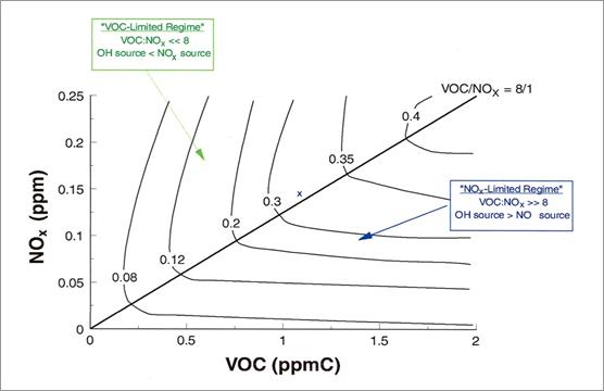
Three primary determinants of ozone chemistry are NOx, VOCs, and sunlight. Ozone is produced by the photolysis of nitrogen dioxide (NO2), creating nitric oxide (NO) and a single atom of oxygen. This atom of oxygen then combines with molecular oxygen (O2) to form ozone (O3). In the absence of VOCs, O3 reacts with NO to re-form NO2, resulting in zero net ozone production; this reaction is referred to as NOx titration. When VOCs, are present, they can react in the presence of sunlight (primarily) to provide radicals which in turn can react with NOto re-form NO2, and compete with the reaction route that consumes O3, leading to net ozone production. Thus, O3 concentrations will rise when sufficient amounts of NOx and VOCs are present along with adequate sunlight. Enhanced ozone levels have a positive feedback on ozone and fine PMformation through the production of the hydroxyl radical leading to organic radicals, organic nitrates and nitric acid. The ratio of ambient concentrations of VOCs to NOx is critically important to the rate of ozone production. The relationship of this ratio to ozone production is fairly well understood (NARSTO, 2000). The Ekma (Empirical Kinetic Modelling Approach) diagram (Figure 7.1), is a simple box model approach to estimate the amount of ozone produced at various levels of VOCs and NOx. The model indicates that, in the absence of large transport of ozone into the region, the VOC to NOx ratio of about 8:1 is optimal for ozone production. If the local ratio falls outside of the optimum range, ozone production is limited by the ability of one species to compete for the available oxidants (primarily OH radicals). This is an important concept in understanding ozone production in the Georgia Basin/Puget Sound airshed. More comprehensive models which include dynamics and transport can give a clearer picture of the effect of control strategies within the air shed.
Figure 7.1. Relationship between NOx, VOCs and ozone, expressed in the form of an EKMA diagram (NARSTO, 2000; Dodge, 1977)
Description of Figure 7.1
Figure 7.1 is an EKMA diagram with VOC concentration (in ppmC) plotted on the x-axis and NOx concentrations (in ppm) plotted on the y-axis. The VOC concentration range is from 0 to 2 ppmC and the NOxconcentration range is from 0 to 0.25 ppm. Also plotted are ozone isopleths at 0.08, 0.12, 0.2, 0.3, 0.35, and 0.4 ppm. A line is also plotted along a VOC/NOx ratio of 8/1. This line runs diagonally from the origin to the upper right corner. The VOC limited regime occurs where VOC/NOx is much less than 8/1 which is the area above the VOC/NOx 8/1 line. Here the OH source is less than the NOx source and the ozone isopleths fall at slightly higher NOx concentrations as VOC concentration increases. The NOx limited regime occurs where VOC/NOx is much greater than 8/1 which is the area below the VOC/NOx 8/1 line. Here the OH source is greater than the NO source and the ozone isopleths fall at slightly decreasing NOx concentrations as VOC concentrations increase.
7.2 Background Ozone
For the purposes of this discussion, background ozone is defined as the ambient level resulting from anthropogenic and natural emissions outside the airshed and natural sources within the airshed. Background ozone is important as a component of local ozone and indicates the lower limit that can be achieved by local reduction efforts.
7.2.1 Sources of Background Ozone
There are three documented sources of background ozone, as described in (Dann et al., 2011): 1) downward mixing from the upper troposphere to the surface, 2) transport of ozone from outside the airshed, and 3) in-situ photochemical production from natural (biogenic methane, NOx, VOC) and transported ozone precursors such as PAN. The major episodic background sources in British Columbia are:
- Intrusions of stratospheric ozone rich air during stratospheric down-folding events (Bovis, 2003)
- Trans-Pacific transport of anthropogenically generated ozone (Jaffe et al., 2004).
- Trans-Pacific transport of ozone generated by bio-mass burning (Keating et al., 2005).
- Locally generated “natural ozone” from lightning and forest fires.
The relative importance of these episodic background sources for British Columbia is quantified in Table 7.1.
| Background Sources | Maximum Ambient Ozone Concentration | Duration of Event | Background Contribution to Ambient | Spatial Extent | Frequency |
|---|---|---|---|---|---|
| Stratospheric Intrusion1 |
30-40 ppb
|
days
|
50-100% (20-40 ppb)
|
regional
|
several times per year
|
| Trans-Pacific Anthropogenic Ozone Episodes2 |
>80 ppb in mid-troposphere
40 ppb near ground |
hours to days
|
50% at mid-troposphere
0-10% on ground (5 ppb) |
regional
|
spring
4 to 6 cases per decade |
| Trans-Pacific Biomass Burning Plumes3 |
96 ppb
|
hours
|
Siberian plume 15% (15 ppb) 50% of “normal” background
|
regional
|
several times per decade
|
| Local Forest Fires4 |
60 ppb
|
days
|
variable, depending on fire location
|
local
|
inter-annual
|
Notes:
1 Bovis (2003)
2 Jaffe et al. (2003)
3 Keating et al. (2005); Bertschi and Jaffe (2005), Bertschi et al. (2004), Jaffe et al. (2004)
4 Based on analysis of Kelowna 2003 event
Description of Table 7.1
Table 7.1 presents the impact of four background sources on ozone in British Columbia.
The first row of the table contains the headers “Background sources”, “Maximum Ambient Ozone Concentration”, “Duration of Event”, “Background Contribution to Ambient”, “Spatial Extent”, and “Frequency”. The first column shows the different background sources being considered. These are:
- Stratospheric Intrusion (reference: Bovis (2003))
- Trans-Pacific Anthropogenic Ozone Episodes (reference: Jaffe et al. (2003))
- Trans-Pacific Biomass Burning Plumes (references: Keating et al. (2005); Bertschi and Jaffe (2005), Bertschi et al. (2004), Jaffe et al. (2004))
- Local Forest Fires (Based on analysis of Kelowna 2003 event)
The second through sixth columns give the details of how each background source type impacts ozone in British Columbia.
For Stratospheric Intrusion Maximum Ambient Ozone Concentration is 30-40 ppb , Duration of Event is days, Background Contribution to Ambient is 50-100% (20-40 ppb), Spatial Extent is regional, and Frequency is several times per year.
For Trans-Pacific Anthropogenic Ozone Episodes Maximum Ambient Ozone Concentration is >80 ppb in mid-troposphere 40 ppb near ground, Duration of Event is hours to days, Background Contribution to Ambient 50% at mid-troposphere 0-10% on ground (5 ppb), Spatial Extent is regional, and Frequency is spring -4 to 6 cases per decade.
For Trans-Pacific Biomass Burning Plumes Maximum Ambient Ozone Concentration is 96 ppb, Duration of Event is hours, Background Contribution to Ambient is Siberian plume 15% (15 ppb) 50% of “normal” background, Spatial Extent is regional, and Frequency is several times per decade.
For Local Forest Fires Maximum Ambient Ozone Concentration is 60 ppb, Duration of Event is days, Background Contribution to Ambient is variable, depending on fire location, Spatial Extent is local, and Frequency is inter-annual.
The intrusion of ozone from the stratosphere to the troposphere was explored by several studies in the Lower Fraser Valley. Bovis (2003) used a beryllium radioisotope (7Be), a tracer for stratospheric ozone and found that this source may contribute 20-40 ppb to short-term peak concentrations of ozone. However, the episodic impact on background concentrations at ground level was found to be relatively small. Moreover, the study did not find an increased frequency of stratospheric-tropospheric exchange (STE) events during the spring, when median ozone concentrations are highest. Stratospheric intrusion events are typically more important at high elevation sites (Dann et al., 2011). Although its effect is not quantified in Table 7.1, it is also possible for ozone from the upper troposphere to descend to the surface under the specific conditions. Vingarzan et al. (2007) found that elevated winter ozone levels of up to 77 ppb were associated with vertical motion coincident with the passage of cold fronts.
Episodic trans-Pacific ozone transport (arising from either biomass burning or anthropogenic combustion sources in Asia) can increase short-term ground level concentrations on the west coast of North America by 5-15 ppb (McKendry, 2006). Jaffe et al. (2004) have shown that the extensive wildfires in Siberia during summer of 2003 likely had a significant impact on the exceedence of the O3standard at Enumclaw, Washington, when the 8-hour average ozone concentrations reached 96 ppb. Of this, 15 ppb was attributed to the Siberian fire plume. Modelling studies suggest that ground-level ozone in the Puget Sound airshed is more sensitive to Asian emissions than other regions in the U.S. (NRC, 2009), on account of being located downwind of these emissions. The contribution of long range transport on ambient ozone levels in the airshed is explored further in Chapter 11, “Transboundary Transport”.
7.2.2 Average and Trends in Background Ozone
Vingarzan (2004) estimated the mean background level in Canada to be in the range of 20-35 ppb, varying seasonally with a spring maximum. This is comparable to the Policy-Relevant Background level of 20-40 ppb in the United States (NRC, 2009). Over the past three decades, the mid-latitude background level in the Northern Hemisphere has been rising by approximately 0.5-2% per year (Vingarzan, 2004). This increase has occurred in spite of declines in peak ozone concentrations in many of the more densely populated areas of the United States due to reductions in local emissions of NOx and non-methane hydrocarbons (NMHC) (U.S. EPA, 2003).
The background level of 20-35 ppb represents approximately 50% of the Canada-Wide Standard for ozone and about 35% of the current U.S. National Ambient Air Quality Standard of 75 ppb. Given the short-term variability in background sources, McKendry (2006) states it is likely that the Canada-Wide Standard will occasionally be exceeded in British Columbia by either background sources alone or the additive effect of locally-produced anthropogenic ozone and background levels.
A more recent investigation was conducted by Chan and Vet (2009) who analysed background ozone at 97 non-urban sites in Canada and the U.S over the period 1997-2006. Clustered back-trajectory analysis was performed to identify the cleanest background air sector for each site. In the Georgia-Basin, background ozone ranged annually from 14 to 24 ppb. Background ozone levels varied seasonally (and diurnally) with concentrations ranging from 22 to 24 ppb in the spring and 15 to 23 ppb in the winter (Dann et al., 2011; Chan and Vet, 2009). Background levels were found to be significantly increasing by 0.28 ppb/year in the spring and 0.72 ppb/year in the summer. Within the margin of error, these values agree with other trends for U.S. west coast background sites, ranging from 0.3 to 0.4 ppb/year (NRC, 2009).
7.3 Seasonal and Diurnal Cycles of Ambient Ozone
7.3.1 Seasonal Cycles
Ozone measurements collected at urban, suburban and rural locations in the airshed provide a good description of variations in the spatial and temporal distribution of ozone concentrations. Commonly, ozone measurements are analysed for the peak summer ozone season in May through September. Because photochemical ozone production depends on heat and sunlight (aside from NOx and VOC precursors), the potential to form ozone reaches a peak during the summer. The highest concentrations of ozone for the year are recorded during this period, which is associated with short-duration peak events or episodes.
Figure 7.2 shows monthly box plots for ozone concentrations at the year-round ozone monitoring sites in the Puget Sound and Surrey East in the Georgia Basin. Some recently discontinued sites with long term records are also shown. As is typical for the region, the highest maximum values occur between May and August and the highest average monthly concentrations occur during the spring. This springtime ozone maximum results from increased ozone production by enhanced UV-dependent photochemical reactions and a seasonal maximum in trans-Pacific transport of ozone and ozone precursors (Vingarzan, 2003). Lower concentrations during the fall and winter are caused by reduced local production due to cooler temperatures and less solar radiation.
Figure 7.2. Box plots of daily 8hour maximum ozone concentrations at year-round sites in the Georgia Basin Puget Sound airshed.
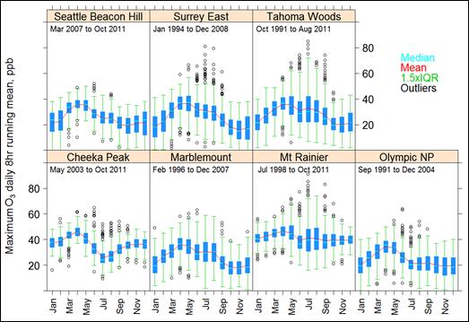
Notes: ”IQR” (blue box) is defined as the inter-quartile range; outliers are not necessarily statistically significant
Description of Figure 7.2
Figure 7.2 shows monthly boxplots of the 8-hour running mean maximum ozone concentration (in ppb) for seven year-round sites in the Georgia Basin-Puget Sound airshed. The median, mean, interquartile range (IQR), 1.5 times the IQR, and any outliers are shown (outliers are not statistically significant).
For Seattle-Beacon Hill there is data from Mar 2007 to Oct 2011. The highest maximum concentration occurs in May (approximately 50 ppb) and the highest average monthly concentrations occur in April and May (approximately 35 ppb). The minimum average monthly concentration occurs from October through February and is approximately 20 ppb.
For Surrey East there is data from Jan 1994 to Dec 2008. The highest maximum concentration occurs in May (approximately 60 ppb) and the highest average monthly concentrations occur in April and May (approximately 40 ppb). The minimum average monthly concentration occurs from October through January and is approximately 15 ppb.
For Tahoma Woods there is data from Oct 1991 to Aug 2011. The highest maximum concentration occurs in July (approximately 75 ppb) and the highest average monthly concentrations occur in April and May (approximately 40 ppb). The minimum average monthly concentration occurs from October through January and is approximately 20 ppb.
For Cheeka Peak there is data from May 2003 to Oct 2011. The highest maximum concentration occurs in April (approximately 60 ppb) and the highest average monthly concentration occurs in April (approximately 45 ppb). The minimum average monthly concentration occurs in July and August and is approximately 25 ppb.
For Marblemount there is data from Feb 1996 to Dec 2007. The highest maximum concentrations occur in July and August (approximately 60 ppb) and the highest average monthly concentration occurs in April (approximately 35 ppb). The minimum average monthly concentration occurs from October through January and is approximately 15 ppb.
For Mt Rainier there is data from July 1998 to Oct 2011. The highest maximum concentration occurs in August (approximately 70 ppb) and the highest average monthly concentrations occur in March and April (approximately 45 ppb). The minimum average monthly concentration occurs in June and is approximately 35 ppb.
For Olympic NP there is data from Sept 1991 to Dec 2004. The highest maximum concentration occurs in May (approximately 45 ppb) and the highest average monthly concentrations occur in April and May (approximately 35 ppb). The minimum average monthly concentration occurs in July through January and is approximately 20ppb.
It is also clear from Figure 7.2 that Mt Rainier and Cheeka Peak display distinctly different patterns from the other sites. Mt Rainier is a high elevation background site (1615 m) that is often decoupled from the boundary layer. The amplitude of the monthly averages is not as pronounced as at the other sites, although high ozone events in the summer months are sometimes observed there due to the influence of forest fires. Cheeka Peak, an elevated coastal background site (478 m), established for the purpose of measuring background levels, advected into the United States over the Pacific Ocean, exhibits the typical spring dominated pattern typical of background sites.
To more closely visualize how ozone compares between different locations, monthly differences between selected sites were examined (Figure 7.3). The seasonal ozone pattern at Beacon Hill and Surrey East during non-summer months is characterized by concentrations below ambient background. This is a consequence of “NOxtitration” in urban areas (see next section). Concentrations at the Surrey site are marginally elevated above those at Beacon Hill in the summer months, as the former is located in a suburban area while the latter is located downtown. Tahoma Woods, located within Mt. Rainier National Park, is at 415 m above sea level. The influence of the urban plume at Tahoma Woods is apparent in the higher O3 levels compared to the Cheeka Peak site during the summer months. Concentrations at Tahoma Woods also are routinely higher than at Beacon Hill (Figure 7.2), probably because of the absence of the above-mentioned NOx titration effect. Tahoma Woods and the now-discontinued Marblemount site in the North Cascades (108 m) showed very similar patterns year round (Figure 7.2), but ozone at Tahoma Woods was above that measured at the Olympic National Park site (427 m) during the summer (monthly median differences are very close to zero from October- May) (not shown). The possible reason is that the Olympic National Park is rarely influenced by urban plumes, unlike Tahoma Woods which is often influenced by urban plumes from the Seattle-Tacoma region. Some urban influences or local ozone production due to enhanced biogenic VOCs are clearly visible in the summer months and coincide with the warmest days with enhanced vertical mixing. Ozone at Mt Rainier is higher than Tahoma Woods during the non-summer months due to its elevation, which results in free tropospheric air being sampled for a significant portion of the time.
Figure 7.3. Monthly differences in daily maximum 8hr ozone levels between selected sites.
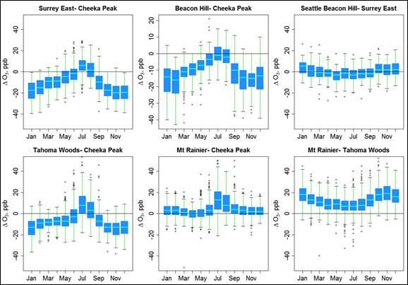
Notes: ”IQR” (blue box) is defined as the inter-quartile range; green whiskers denotes 1.5*IQR; aqua blue bar denotes the median difference; outliers (black circles) are not necessarily statistically significant
Description of Figure 7.3
Figure 7.3 shows boxplots of differences in 8 hour ozone levels for six pairs of air monitoring stations in the airshed. For each pair of stations being compared, the x-axis shows the month and the y-axis shows the difference in ozone concentration (in ppb).
For Surrey East - Cheeka Peak the median ozone concentration difference ranges from approximately -20 ppb in November, December, and January to approximately +5 ppb in July. All differences are negative except for July and August.
For Beacon Hill - Cheeka Peak the median ozone concentration difference ranges from approximately --15 ppb for October through February to approximately 0 ppb in July. All differences are negative.
For Seattle Beacon Hill - Surrey East the median ozone concentration difference ranges from just below zero in May through August to approximately +5 ppb in January. All differences are within +-5ppb of zero.
For Tahoma Woods - Cheeka Peak the median ozone concentration difference ranges from approximately -15 ppb in October through January to approximately +5 ppb in July. All differences are negative except for July and August.
For Mt Rainer - Cheeka Peak the median ozone concentration difference ranges from 0 ppb in April and MAy to approximately +10 ppb in July. All differences are greater than 0 ppb.
For Mt Rainer - Tahoma Woods the median ozone concentration difference ranges from approximately +5 ppb in June through August to approximately +20 ppb in November through January. All differences are greater than 0 ppb.
7.3.2 Diurnal Cycles
Ozone concentrations follow a typical photochemically-produced diurnal variation. Figure 7.4 shows ozone data from the Beacon Hill site in Seattle. Peak concentrations occur in the mid-afternoon, with minimum values observed in the early morning hours.
Because it takes time for ozone to form, the highest ozone concentrations are often observed at sites downwind of precursor emissions. As such, the highest ozone concentrations do not usually occur in urban areas where ozone precursors are emitted. Another reason for the absence of high ozone levels in urban areas is the absence of major ozone-precursor source areas upwind of the Puget Sound/ Georgia Basin sites. This is an important difference between this region and the North American east coast. Puget Sound’s highest ozone concentrations are typically observed near Enumclaw, to the southeast of Seattle, in the direction of the prevailing winds during high ozone events. In urban areas it is also common to see ozone concentrations fall to near zero at night, as shown in Figure 7.4, due to reactions of ambient ozone with NO emissions (the NOx titration effect) and the absence of photochemical ozone production.
Figure 7.4. Diurnal variation of ozone at Beacon Hill Seattle
Notes: Based on hourly average concentrations (AIRS Station 53-033-0080)
Description of Figure 7.4
Figure 7.4 is a bar chart showing hourly average ozone concentrations at Beacon Hill in Seattle. The x-axis shows hour of day from 0000 to 2400 hours and the y-axis shows ozone concentration from 0 to 60 ppb. The median, mean, 25-75 percentile range, 5-95 percentile range, and 98thpercentile value are plotted. There is a note that the plot is based on hourly average concentrations (AIRS Station 53-033-0080).
At 0000 hours the median and mean are approximately 16ppb with the median slightly higher. The 25-75 percentile range is approximately 6-24ppb, The 5-95 percentile range is approximately 2-35ppb, and the 98th percentile is approximately 39ppb. There is a decrease in all values until a minimum is reached at 0600 hours when the median is approximately 9ppb, the mean is approximately 12ppb , the 25-75 percentile range is approximately 2-17ppb, The 5-95 percentile range is approximately 2-29ppb, and the 98th percentile is approximately 34ppb. There is then a steady increase until a maximum is reached at 1400 hours when the mean and median are approximately 27ppb. The 25-75 percentile range is approximately 20-34ppb, and the 5-95 percentile range is approximately 7-45ppb. The maximum 98thpercentile is approximately 50ppb and occurs at 1500 hours. After 1500 hours there is a steady decline through 2000 hours when the mean is approximately 15ppb, the median is approximately 14ppb. The 25-75 percentile range is approximately 2-22ppb, the 5-95 percentile range is approximately 2-34ppb, and the 98thpercentile value is approximately 39ppb. At 2400 hours the mean and median are approximately 16ppb, the 25-75 percentile range is approximately 5-23ppb, the 5-95 percentile range is approximately 2-35ppb, and the 98th percentile value is approximately 38ppb.
Many rural sites exhibit a similar mid-afternoon O3 maximum, although the lack of NOx emissions allows overnight ozone values to remain at 10 to 20 ppb or higher. The diurnal pattern of ozone concentrations can be modified at rural sites through the transport of ozone and ozone-forming precursors. Ozone concentrations can reach maximum values during the evening and overnight, depending on the nature of the ozone transport and the proximity of the site to emission sources. For example, ozone concentrations at Paradise on Mount Rainier have been observed between 40 and 70 ppb overnight, often with peaks in the morning rather than the afternoon (Brace and Peterson, 1998).
Mountain monitoring sites such as Paradise on Mount Rainier and nearby White Pass in the Cascades show little diurnal fluctuation in ozone concentrations and can experience moderate to high levels of ozone throughout the day in the summer (Krzyzanowski et al., 2006). Studies at Mount Rainier show increasing ozone exposure with altitude (Brace and Peterson, 1998). This is likely due to increased exposure to free tropospheric ozone. Therefore high-elevation areas of the airshed may experience higher overall ozone levels than either urban or suburban sites where the highest peak levels are observed. This phenomenon makes sensitive alpine ecosystems especially at risk to damage from chronic exposure to ozone (Krzyzanowski et al., 2006). See Chapter 12, Deposition and Ecological Impacts for more information on ozone effects on sensitive ecosystems.
Occasionally, episodes of high ozone concentrations will be sustained for two days to over a week. These summer-time smog episodes receive considerable attention due to their impacts on human health and visibility. Meteorological conditions favoring stagnant surface level conditions and subsidence inversions are the main factors dictating the duration and intensity of ozone episodes, as discussed in Chapter 3, “Air Quality and Weather”. Under stagnant meteorological conditions, ozone and precursors become trapped, leading to an increase in ozone that can build on the previous days’ precursor emissions. These conditions usually affect both the Puget Sound and the Georgia Basin airsheds simultaneously and can result in exceedences of ambient ozone standards.
7.4 Ambient Ozone Levels Compared to Standards and Objectives
Ozone standards and objectives provide decision makers with a benchmark for assessing ozone levels in their jurisdiction, thereby informing decisions on remedial or preventative actions. They can also be used to compare the air quality between airsheds and areas within airsheds. Ozone concentrations in many areas within the Georgia Basin/Puget Sound airshed remain below national standards and regional objectives. However, some locations with low precursor emissions experience periodic exceedences, even while ozone levels at sites with high precursor emissions remain below the standards.
Beacon Hill in Seattle and Robson Square in downtown Vancouver are good examples of sites in areas of significant precursor emissions where the concentrations of ozone are well below air quality standards (Figure 7.5 and Figure 7.6). Downwind of these sites, transport contributes a substantial component of local ozone precursors (especially NOx). As a result, ozone levels downwind are much closer to ambient air quality standards than are concentrations at urban sites. In Figure 7.5, Enumclaw is shown to have higher ozone levels than upwind Seattle. Similarly, in Figure 7.6, sites in the eastern Lower Fraser Valley (Abbotsford, Chilliwack, Hope) have higher ozone levels than the more urban upwind sites in the west (Kitsilano, Robson, Rocky Point).
Downwind of Seattle, the Enumclaw, WA, site experiences ozone concentrations that exceed the current U.S. ozone standard of 75 ppb (Figure 7.5). Design values (three year average of the annual 4th highest 24-hr maximum calculated from 8-hour running means) for ozone concentrations at Enumclaw have remained between 70 and 75 ppb over the last decade.
In the Lower Fraser Valley, the highest ozone concentrations occur in the eastern portion of the LFV, as a result of the sea-breeze flow concentrating precursor emissions towards its eastern extent (Brook et al., 2011). Consequently, several stations in the eastern WISE have come very near the Canada-Wide Standard (CWS) metric over the past few years (Figure 7.6), including Hope, which exceeded the CWS between 2003 and 2006.
The contrast between Robson Square and Hope is similar to that of Seattle and Enumclaw. A densely urban site, Robson Square is exposed to significant levels of vehicle emissions, experiencing the highest annual NO2 levels in the WISE (24 ppb), and exceeding Metro Vancouver’s annual air quality objective for NO2 of 22 ppb (Metro Vancouver, 2010). Low night-time concentrations of O3 indicate significant titration by NO at this site. Conversely, Hope experiences NOx levels typical of rural-impacted locations in British Columbia, and its anthropogenic VOC levels are relatively low compared to that of more urban sites (Brook, et al., 2011).
Figure 7.5. U.S. EPA ozone standard metric at Seattle and Enumclaw in the Puget Sound
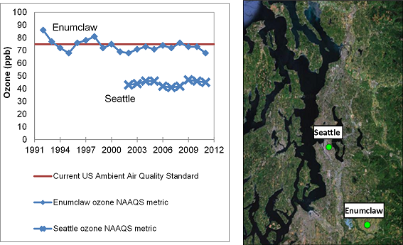
Notes: 3 year running means of 4th highest yearly 24 hour maximum calculated from 8 hour running means (AIRS Station 53-033-0080 for Seattle) (AIRS Station 53-033-7001 and 53-033-0023 for Enumclaw, as site was shifted by approximately 2 miles south in 2000 to a comparable location)
Description of Figure 7.5
Figure 7.5 has two parts. On the right is a satellite image showing the Puget Sound area with the locations of Seattle and Enumclaw marked by circles. On the left is a plot with the years 1991 through 2012 on the x-axis and ozone concentration from 0 to 100 ppb on the y-axis. A horizontal line at 75 ppb marks the current US Ambient Air Quality Standard. The data shown are 3 year running means of 4th highest yearly 24 hour maximum calculated from 8 hour running means using AIRS Station 53-033-0080 for Seattle and AIRS Station 53-033-7001 and 53-033-0023 for Enumclaw (The Enumclaw site was shifted by approximately 2 miles south in 2000 to a comparable location). For Seattle there is data for 2002 through 2011 with all values falling between 40 and 50 ppb and no upward or downward trend in the data. For Enumclaw there is data for 1992 to 2011 with the 1992 value falling at approximately 85 ppb and all other values falling between 65 and 80 ppb. Again, there is no upward or downward trend in the data.
A recent analysis using 20 years of data by Steyn et al. (2011) describes the spatial pattern of ozone during episodic conditions in the Lower Fraser Valley of BC. Study findings describe a high concentration centroid positioned over the eastern extent of the WISE in the area of Chilliwack and Hope, which is consistent with the spatial pattern of current observations. This centroid has shifted since the 1980s, at which time it was positioned over the central part of the WISE and closer to the north shore mountains. This shift may have occurred due to changes increasing precursor emissions in the central part of the LFV. The study also found strong ozone titration in and around the urban source region (such as observed at Robson Square), with higher values downwind, as shown for the eastern WISE in Figure 7.6. The study also suggests that precursor build-up prior to the exceedence day plays an important role in the spatial ozone pattern on exceedence days.
Figure 7.6. Canada Wide Standard ozone standard metric for six sites in the Lower Fraser Valley
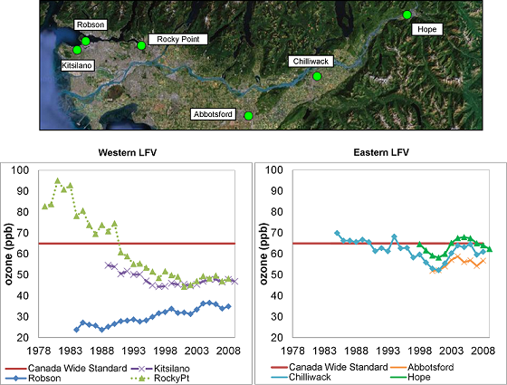
Notes: 3 year running means of 4th highest yearly 24 hour maximum calculated from 8 hour running means
(NAPS Stations, west to east: 100118, 100112, 100111, 101003, 101101, 101401)
Description of Figure 7.6
Figure 7.6 is composed of three parts. The upper panel is a satellite image of the Lower Fraser Valley with the locations of the Robson, Kitsilano, Rocky Point, Abbotsford, Chilliwack, and Hope NAPS air quality monitoring stations marked by circles. Two plots, one on the lower left and one on the lower right, have the years 1975 through 2010 on the x-axis and ozone concentration from 20 to 100 ppb on the y-axis. Both also have a horizontal line at 65 ppb marking the Canada Wide Standard. On the left there is data for the Western WISE stations (Robson, Kitsilano, and Rocky Point) and on the right there is data for the Eastern WISEstations (Abbotsford, Chilliwack, and Hope). The data shown is 3 year running means of 4th highest yearly 24 hour maximum calculated from 8 hour running means (NAPS Stations, west to east: 100118, 100112, 100111, 101003, 101101, 101401).
For the Robson station there is data for 1984 to 2009. In 1984 the ozone concentration was approximately 23 ppb which rose steadily to a concentration of approximately 33 ppb in 2009. For the Kitsilano station there is data for 1990 through 2010. In 1990 the ozone concentration was approximately 55 ppb, this declined steadily to approximately 45 ppb in 1997 and then remained between 45 and 50 ppb through 2010. For the Rocky Point station there is data for 1979 through 2010. In 1979 the ozone concentration was approximately 80 ppb. This rose to a peak of 95 ppb in 1981 and then declined to approximately 45 ppb in 2001. Between 2001 and 2010 the concentration remained between 45 and 50 ppb.
For the Abbotsford station there is data for 2000 through 2009. In 2000 the ozone concentration was just above 50 ppb. This rose to a peak of approximately 60 ppb in 2004 and then remained between 55 and 60 ppb through 2009. For the Chilliwack station there is data for 1985 through 2010. In 1985 the ozone concentration was approximately 70 ppb. Between 1986 and 1995 the concentration remained at approximately 65 ppb before falling to just above 50 ppb in 1999. The concentration then returned to 65 ppb for 2003 through 2005 before falling to approximately 60 ppb for 2006 through 2010. For the Hope station there is data for 1998 through 2010. From 1998 to 2001 the ozone concentration fell steadily from 65 ppb to approximately 55 ppb before rising to just below 70 ppb in 2005. From 2005 to 2010 there was steady decline to approximately 60 ppb.
7.5 Ozone Episodes
Although exceedences of ozone standards are most commonly observed in Hope and Enumclaw, the exceedence area can be large during regional ozone episodes. Ozone episodes typically occur during July and August when the combined effect of ultraviolet radiation, temperature and regional stagnation are highest. During episodic conditions, hourly ozone concentrations sometimes rise over 80 ppb and occasionally over 100 ppb.
Between 2001 and 2008, there were a total of three regional-scale ozone episodes in the Lower Fraser Valley. A regional episode was defined as a minimum of four out of twelve monitoring sites registering a daily 8-hour ozone level greater than 65 ppb. These episodes are summarized in Table 7.2.
| Lower Fraser Valley Regional Episode Criteria | Total No. of Regional Scale Episodes | Notable Episode Dates | No. of Sites Recording Max 8h Ozone > 65 ppb |
Max. 8h Ozone (ppb) |
|---|---|---|---|---|
| 4 or more Sites > 65 ppb (total Sites 12) |
3
|
20-Jun-2004
|
4
|
69
|
|
16-May-2006
|
5
|
73
|
||
|
17-May-2008
|
4
|
66
|
Description of Table 7.2
Table 7.2 is a summary of regional scale ozone episodes in the Lower Fraser Valley for the Period 2001-2008.
The first row of the table contains the headers “Lower Fraser Valley Regional Episode Criteria”,” Total No. of Regional Scale Episodes”,” Notable Episode Dates”,” No. of Sites Recording Max 8h Ozone > 65 ppb”, and “Max. 8h Ozone (ppb)”. The first column gives the Lower Fraser Valley Regional Episode Criteria which is 4 or more Sites > 65 ppb (total Sites 12). The second column gives the Total No. of Regional Scale Episodes which is 3. The third column has three rows giving notable episode dates, and the fourth and fifth columns give the details of these episodes which are the number of sites recording maximum 8h ozone > 65 ppb and the maximum 8h ozone (ppb)).
In the Puget Sound, the highest ozone levels in recent history occurred during the July 22-28, 1998 episode. One-hour average ozone concentrations as high as 140 ppb were observed downwind of Seattle and 8-hour average concentrations reached 111 ppb (Lamb et al., 2006). More recently, from 2007 through 2009, 1-hour maximum ozone concentrations were as high as 114 ppb, and 8-hour average maxima reached 91 ppb.
7.6 Ozone Trends in the Georgia Basin
Trends in ambient ozone levels were investigated for the western and eastern Lower Fraser Valley (LFV), respectively, for the period 1991-2012, using the fitted slopes of various simple linear regressions performed on different parts of the statistical distribution, as shown in Figure 7.7. The 1991-2012 period was chosen in order to capture the most current emission regime, including the implementation of federal regulations on vehicles and fuels and the Air Care program in the LFV. The western and eastern WISE were investigated separately to distinguish between the western source areas and the downwind eastern areas. In the western LFV, ozone trends were positive (p<0.05) up to the 95th percentile, while hourly ozone maxima showed no trend. In the eastern LFV, ozone trends were positive (p<0.05) up to the 90thpercentile, and ozone maxima showed a statistically significant decreasing trend. In spite of the decreasing trend in the maxima in the eastern part of the LFV, exceedences of the Canada Wide Standard, continued to occur at Hope, located at the eastern apex of the WISEthroughout this period. As a whole, the ozone trends observed in the WISE are consistent with a VOC-limitation in the western portion of the airshed and a mixed VOC-NOx limitation regime in the eastern portion (see Section 7.7 for a more in depth analysis of ozone reactivity in the WISE airshed). Increasing trends in the lower part of the O3 distribution have been noted elsewhere (Jenkin, 2008) and are believed to largely reflect declining NOx levels (decreased titration) and possibly increases in background ozone (Royal Society, 2008).
Figure 7.7. 1991-2012 trends in hourly ozone concentration in the Lower Fraser Valley
Notes: Simple linear regression ofaverage hourly data for the period 1991-2012. All WISE stations included except Robson. West-east divide is at the Surrey-Langley border. Statistically significant (p<0.05) increasing trends indicated in red and decreasing trends indicated in blue.
Description of Figure 7.7
Figure 7.7 is divided into two plots, one for the Western WISE on the top and one for the Eastern WISE on the bottom. On both x-axes are the years 1991 through 2012 and on both y-axes are ozone concentrations from 0-100 ppb. There is a note that these plots show simple linear regression of average hourly data for the period 1991-2012, that all WISE stations are included except Robson, that the west-east divide is at the Surrey-Langley border, and that statistically significant (p<0.05) increasing and decreasing trends are indicated.
In the upper panel (Western LFV) data for the 10th, 25th, 50th, 75th, 90th, and 95th percentiles are shown, as well as data for the maximum concentrations. For the 10th percentile there is a significant increasing trend from approximately 2-5 ppb. For the 25th percentile there is a significant increasing trend from approximately 5-10 ppb. For the 50thpercentile there is a significant increasing trend from approximately 10-15 ppb. For the 75th percentile there is a significant increasing trend from approximately 20-25 ppb. For the 90th percentile there is a significant increasing trend from approximately 30-35 ppb. For the 95thpercentile there is a significant increasing trend from approximately 35-39 ppb. For the maximum there is no significant trend and the concentration is stable just below 65 ppb.
In the lower panel (Eastern LFV) data for the 10th, 25th, 50th, 75th, 90th, and 95th percentiles are also shown, as well as data for the maximum concentrations. For the 10th percentile there is a significant increasing trend from approximately 0-5 ppb. For the 25th percentile there is a significant increasing trend from approximately 5-10 ppb. For the 50th percentile there is a significant increasing trend from approximately 15-19 ppb. For the 75th percentile there is a significant increasing trend from approximately 25-30 ppb. For the 90th percentile there is a significant increasing trend from approximately 35-39 ppb. For the 95th percentile there is no significant trend and concentrations are stable around 40 ppb. For the maximum there is a significant decreasing trend from approximately 80-70 ppb.
Table 7.3 presents seasonally and meteorologically adjusted ozone trends at Saturna Island regional site. Saturna Island is one of the Gulf Islands in the Strait of Georgia, situated at the confluence of the northwest-southeast and northeast-southwest arms of the Strait. There are very few direct anthropogenic sources on the island, although the site is at times influenced by plumes from marine vessel traffic (McLaren et al., 2010). All trends show ozone to be increasing, although the more recent trends from 1997 to 2006 suggest a slowing down of this trend.
| Ozone Trend Metric | Adjusted Ozone Trend 1990-2006 (ppb yr-1) |
Adjusted Ozone Trend 1997-2006 (ppb yr-1) |
|---|---|---|
| 24-Hour Average |
0.56
|
0.26
|
| Daytime Average |
0.74
|
0.26
|
| Night-time Average |
0.49
|
0.31
|
Notes: Values in bold are statistically significant at p<0.05. Trends are meteorologically and seasonally adjusted
from observations by CAPMoN/NAPS site 102001 (178 m elevation). Daytime averages: 10:00-18:00hrs; Night-time averages: 20:00-4:00 hrs. Source: (Dann et al., 2011).
Description of Table 7.3
Table 7.3 gives adjusted ozone trends at Saturna Island for the periods 1990-2006 and 1997-2006.
The first row of the table contains the headers “Ozone Trend Metric”, ”Adjusted Ozone Trend, 1990-2006 (ppb yr-1)”, and Adjusted Ozone Trend, 1997-2006 (ppb yr-1)”. The first column gives the ozone trend metrics which are 24-hour average, daytime average, and nighttime average. The second column gives the adjusted ozone trend for 1990-2006. The third column gives the adjusted ozone trend for 1997-2006.
7.7 Ozone Production Regime in the Canadian Lower Fraser Valley
Local ozone control policies need to take into consideration the ozone production regime, which is generally classified as either VOC-limited or NOx-limited (referring to the pollutant that limits the rate of ozone production as described in Figure 7.1.
7.7.1 Ambient Data Analysis Results
Vingarzan and Schwarzhoff (2010) examined ozone reactivity in the Lower Fraser Valley by analysing average warm season VOC/NOx ratios from ten NAPS stations with data extending back to the early 1990s. They found that on average, VOC limitation, defined by VOC/NOx ratios below 8, was observed in various degrees at most sites in the WISE (Figure 7.8). Two sites in the proximity of oil refineries were found to be NOx limited, Hastings and Kensington (not shown). Rocky Point is close to the VOC/NOx ridgeline depicted in Figure 7.9, however this site is influenced by fugitive VOC emission from petroleum tanks located in its proximity. A trend analysis indicated that VOC/NOx ratios declined since 1989. The majority of this decline in VOCs and NOx occurred during the early 1990s, coinciding with federally mandated improvements in vehicles and fuels and the onset of the provincial Air Care program in the Lower Fraser Valley.
Figure 7.8 Average total VOCs, NOx, and VOC/NOx Ratios in the Lower Fraser Valley.
Notes: Based on average concentrations for April to September, 1998-2007(Vingarzan and Schwarzhoff, 2010).
Monitoring Stations are in order of West to East.
Description of Figure 7.8
Figure 7.8 is a bar chart showing the VOC/NOx ratio and average VOC and NOx concentration (in ppb) for the NAPS air quality stations at Vancouver Airport, Richmond South, Robson, Burnaby South, Rocky Point, Surrey East, Chilliwack, and Hope. There is a note that the data is based on average concentrations for April to September, 1998-2007 (Vingarzan and Schwarzhoff, 2010). The stations are listed from west to east.
At Vancouver Airport the average VOC/NOx ratio was just above 2, the average VOCconcentration was approximately 2.5 ppb, and the average NOx concentration was approximately 1 ppb.
At Richmond South the average VOC/NOx ratio was just below 4 ppb, the average VOCconcentration was approximately 2.75 ppb, and the average NOx concentration was approximately 0.75 ppb.
At Robson the average VOC/NOx ratio was approximately 2.5 ppb, the average VOCconcentration was approximately 5 ppb, and the average NOx concentration was approximately 2 ppb.
At Burnaby South the average VOC/NOx ratio was approximately 2.5 ppb, the average VOCconcentration was approximately 2.25 ppb, and the average NOx concentration was approximately 0.75 ppb.
At Rocky Point the average VOC/NOx ratio was approximately 5.5 ppb, the average VOCconcentration was approximately 5 ppb, and the average NOx concentration was approximately 1 ppb.
At Surrey East the average VOC/NOx ratio was approximately 3.5 ppb, the average VOCconcentration was approximately 1.5 ppb, and the average NOx concentration was approximately 0.5 ppb.
At Chilliwack the average VOC/NOx ratio was approximately 2 ppb, the average VOCconcentration was approximately 1.75 ppb, and the average NOx concentration was approximately 1 ppb.
At Hope the average VOC/NOx ratio was approximately 1.25 ppb, the average VOCconcentration was approximately 0.75 ppb, and the average NOx concentration was approximately 0.5 ppb.
7.7.2 Modelling Results
A recent retrospective modelling study over a 20 year period (1985-2005) was undertaken by Steyn et al. (2011) to examine ozone formation in both the Canadian and U.S portions of the Lower Fraser Valley (LFV). This study analysed model simulations of four ozone episodes (each four days in length), using a modelling system that consisted of three major components: the Weather Research and Forecasting (WRF v3.1) meso-scale numerical weather prediction system; the Sparse Matrix operator Kernel Emissions modelling system (SMOKE v2.5); and the Community Multi-scale Air Quality modeling System (CMAQ v4.7.1). The four episodes were chosen to capture the local (meso-scale) meteorological variability generally observed during summertime ozone exceedences in the LFV.
On many of the simulated days, the model showed that the highest ozone concentrations occurred outside of the area sampled by the fixed monitoring network and along the numerous tributary valleys of the LFV. Model output was compared from each of the four events under first the 1985-level emissions and then the 2005-level emissions. Results indicate that that during these episodes, the ozone ridgeline, which separates NOx sensitive from the VOC sensitive regions, has moved westward and southward during the 1985-2005 timeframe (Figure 7.9). The study also found that during peak ozone conditions the eastern part of the WISE around Chilliwack has generally shifted from being VOC-limited to NOx-limited over the last 20 years, as shown in Figure 7.9. However, the ozone ridgeline was found to be sensitive to meteorology and showed significant variability within and between ozone episodes, indicating a mixed VOC/NOx sensitivity around the centre of the LFV. In addition, the study found that the ozone production efficiency with respect to NO has likely increased in the eastern part of the valley, which may have offset some and perhaps all of the NOx emissions reductions achieved in the airshed. The change in ozone sensitivity, along with the increased ozone production efficiency, appears to have changed the shape of the observed diurnal ozone profile to one that is less peaked around the daily maximum, slightly broader and showing less nighttime titration, as shown in Figure 7.10. These factors may be contributing to increased 8-hour averaged ozone concentrations, even if 1-hour averaged concentrations have not increased. In addition, trajectory modelling suggested that emissions and ozone from the Puget Sound region do not directly impact WISE air quality during summertime ozone episodes. The study also estimated that for every 10 ppb increase in background ozone concentration, a roughly 3.0 ppb increase in 8-hour ozone concentrations would be observed.
Figure 7.9 Modelled maximum 8-hr average ozone exposure contours (in 5 ppb increments) under 1985 emissions and 2005 emissions.
a) 1985 emissions
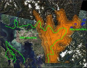
b) 2005 emissions
Notes: Also shown is the predicted VOC/NOx ridgeline based on the modelled [O3]/[NOy] ratio (green line) and the fixed monitoring network station locations (green dots). Regions above 60 ppb are outlined in contours (orange).
Simulation is based on day 3 of the Cluster I simulations, which uses June 2006 meteorology (Steyn et al., 2011).
Description of Figure 7.9
Figure 7.9 has two panels each consisting of a satellite image of the Lower Fraser Valley superimposed with the model results for 8-hr average ozone exposure and the predicted VOC/NOx ridgeline (based on the modelled [O3]/[NOy] ratio). Also shown are the fixed monitoring network station locations. There is a note that the simulation is based on day 3 of the Cluster I simulations, which uses June 2006 meteorology (Steyn et al., 2011).
In the left panel the results under 1985 emissions are shown. In this case the VOC sensitive region includes most of the Lower Fraser Valley. The VOC/NOx ridgeline runs from the Strait of Georgia up the east shore of Howe Sound as far north as Anvil Island and along the North shore. The VOC sensitive region includes the southern part of Indian Arm, Pitt Lake and extends as far east as Agassiz. The VOC/NOx ridgeline then runs southwest to Bellingham Bay. The Southern Gulf Islands are included in the NOx sensitive region while the remainder of Vancouver Island is in the VOC sensitive region. Also shown are ozone exposure contours at 60, 65, 70, 75, and 80 ppb. The 60 ppb contour runs north from Burlington to Stave Lake then turns east and includes the WISE tributary valleys to the north. It extends eastward to the Coquihalla region and southeast just to the west of Mt Baker. The 80 ppb contour encompasses the eastern end of the WISE south of Harrison Lake. The contours are evenly spaced, but are most closely spaced in the east and are less steep in the west.
In the right panel the results of the model under 2005 emission are shown. In this case the VOC/NOx ridgeline has shifted to the west of Chilliwack and now just skirts the northern edge of the WISE without including any of the mountainous areas to the north. The eastern WISE along the 49th parallel has also shifted from a VOC to NOx sensitive regime. In the 2005 emission case only the 60 ppb ozone exposure contour occurs. The area enclosed by the contour is in the NOx sensitive area at the far eastern edge of the WISE and includes the area to the south and east of Harrison Lake, but not extending as far as Hope.
Figure 7.10 The change in the modelled diurnal ozone cycle Chilliwack, B.C from 1984-1990 to 2000-2006.
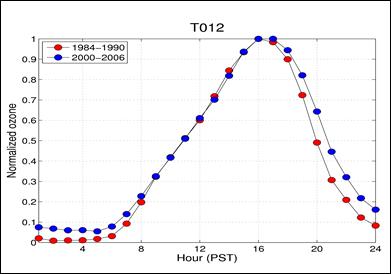
Description of Figure 7.10
Figure 7.10 is a plot of normalized ozone (from 0 to 1) as a function of hour of day in PST. Two traces are shown, both for Chilliwack, BC. The first is for the years 1984-1990 and the second is for 2000-2006. The first trace remains below 0.05 until 0700 and then rises steadily to 1.0 at 1600. It begins to decline at 1700 and falls back to 0.1 by 2400. The second trace remains between 0.05 and 0.1 until 0700 and then rises steadily to 1.0 at 1600. It remains at 1.0 through 1700 and then falls to just over 0.15 by 2400. The normalized ozone values are the same for both traces from 0900 to 1600, but the 2006-2006 trace shows consistently higher normalized ozone from 1600 to 2400, resulting in a broadened profile.
The combined results of the Vingarzan and Schwarzhoff (2010) and Steyn et al., 2011, as well as a recent EC-UBC study (unpublished) indicate the WISE is VOC limited most of the time, with the exception of high ozone episodes (O3 levels above the 95thpercentile) (see Figure 7.7), when NOx limitation occurs in the eastern portion of the airshed. According to the Empirical Kinetic Modeling Approach (EKMA) model depicted in Figure 7.1, in the VOC limited western LFV, additional VOCreductions would help reduce ozone levels on all days, helping to reduce exposure at all percentiles of the ozone distribution. In contrast, because the eastern WISE has a mixed O3 reactivity regime, a more tailored approach to abatement would be required there. Such an approach would involve a focus on VOC reductions on most days of the year (for ozone levels up to the 95th percentile) and additional NOxreductions when ozone levels exceed the 95thpercentile.
7.8 Ozone Trends in the Puget Sound
In the Puget Sound, long term trends in ambient ozone levels were investigated using the fitted slopes of simple linear regressions. Seasonal decomposition was performed on monthly means of the maximum daily 8hr average concentrations collected at several year-round sites. These seasonally adjusted trends were fitted using ordinary least squares (OLS) regression models described in Jaffe and Ray (2007).
Figure 7.11 shows the long term trend at each site resulting from the seasonal decomposition algorithm and the OLS trend line. All sites (with the exception of Mount Rainier) registering a significant trend (p < 0.05) show an increase of about 0.3 ppb/yr, which is in close agreement with the trend at several background sites in the western U.S. (Jaffe and Ray, 2007). The observed reductions of ozone at Mount Rainier are mostly driven by a decline just before 2005. This approximately coincides with the NOxcontrols implemented at the TransAlta Centralia Power Plant, which is thought to be the most likely NOx source that could affect ozone at Mount Rainier.
Figure 7.11. Long term trends from de-seasonalized monthly means of the maximum daily 8hr average ozone concentrations at several year-round sites in the Puget Sound.
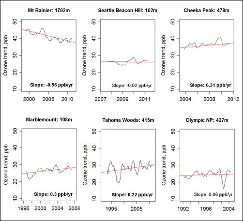
Notes: The temperature term was not included in the linear model as the results made little difference to the magnitude of the long term trend. Statistically significant trends indicated in bold for p<0.05. This analysis is mostly applicable to the background sites, but Seattle Beacon
Hill is included for comparison purposes.
Description of Figure 7.11
Figure 7.11 has six panels showing long-term ozone trends in the Puget Sound area. In all cases the x-axis shows year and the y-axis shows ozone concentration from 10 to 50 ppb. The data and fitted trend line are both shown.
Data for Mt Ranier is in the top left. It is indicated that Mt Ranier is at 1782 m and there is data for 1999-2011. There is a decrease from approximately 45 to 40 ppb and the trend line has a slope of -0.56 ppb/year. This was a statistically significant trend.
Data for Seattle Beacon Hill is in the top middle. It is indicated that Seattle Beacon Hill is at 102 m and there is data for 2007-2011. The concentration is steady just above 25 ppb and the trend line has a slope of -0.02 ppb/year.
Data for Cheeka Peak is in the top right. It is indicated that Cheeka Peak is at 478 m and there is data for 2004-2011. There is an increase from just below to just above 35 ppb and the trend line has a slope of 0.31 ppb/year. This was a statistically significant trend.
Data for Marblemount is in the bottom left. It is indicated that Marblemount is at 108 m and there is data for 1996-2008. There is an increase from just below to just above 25 ppb and the trend line has a slope of 0.3 ppb/year. This was a statistically significant trend.
Data for Tahoma Woods is in the bottom middle. It is indicated that Tahoma Woods is at 415 m and there is data for 1994-2011. There is an increase from approximately 25 to 30 ppb and the trend line has a slope of 0.22 ppb/year. This is a statistically significant trend.
Data for Olympic NP is in the bottom right. It is indicated that Olympic NP is at 427 m and there is data for 1992-2004. The concentration is steady just below 25 ppb and the trend line has a slope of 0.06 ppb/year.
The figure has a note that the temperature term was not included in the linear model as the results made little difference to the magnitude of the long term trend. Statistically significant trends indicated for p<0.05. This analysis is mostly applicable to the background sites, but Seattle Beacon Hill is included for comparison purposes.
7.9 Ozone Production Regime in the Puget Sound
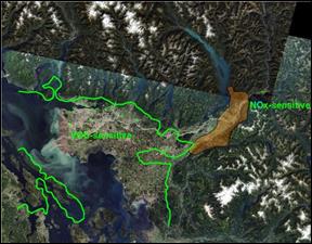
Although an ambient data analysis cannot be performed for the Puget Sound due to limited NOx and NOy, measurements (Arnold et al, 2006), several modelling studies have attempted to characterize ozone chemistry in this airshed. A recent modelling study by (Xie et al., 2011) suggests that the dense urban areas and associated polluted airsheds west of the Cascades are both VOC-limited; preliminary investigation by WA DOE of the VOC/ NOx ratio in the regional forecast model (AIRPACT) emissions inventory at a 12km resolution also suggest VOClimitation closer to urban areas in Western Washington, progressing to NOx limitation further afield, as shown in Figure 7.12. Although these results are in line with ambient data from the Canadian LFV, and make sense with respect to the geographical characteristics of emissions in the Puget Sound, they must be verified with ambient observations.
Figure 7.12. VOC/ NOx ratio from AIRPACT inventory, on a high O3 day.
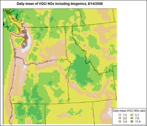
Notes: The 2008 emissions inventory was used in the model.
Description of Figure 7.12
Figure 7.12 is a line map encompassing an area from the Pacific Ocean in the west to the western border of Wyoming in the east, and from Campbell River BC in the north to Eureka California in the south. The map is colored by daily mean VOC/NOx ratio in increments of 1.5, 2.2, 3.4, 5.1, 7.6, and 11.4.
In general the VOC/NOx ratio is quite spatially inhomogeneous. For most of the eastern and southern shore of Puget Sound the ratio is 1.5 and only rises as high as 2.2 on the western slope of the Cascades. Along the west coast of Washington State the value is at 2.2 with the exception of the Olympic Peninsula whose inland areas have ratios of up to 7.6.
In Canada, the Lower Fraser Valley has a ratio of 2.2, except at the very eastern end where the ratio goes up to 5.1. The Strait of Juan de Fuca has a ratio of 2.2 while the Strait of Georgia has a ration of 5.1. Most of Vancouver Island has a ratio of 7.6 to 11.4. The very southern end of Vancouver Island has a ratio of 5.1. The Sunshine coast and the islands to the north of the Strait of Georgia have ratios of 7.6 to 11.4.
In the remainder of the map area the VOC/NOx ratio is also very inhomogeneous. Areas with low ratios include coastal Oregon, the north coast of California, along the Columbia River, and some patches in southern Idaho. Higher ratios occur in central Idaho, central Oregon, and northern inland portions of California.
7.10 Chapter Summary
Ground level ozone is an environmental and health concern in the Georgia Basin/Puget Sound airshed. In this chapter, ozone pollution was described by investigation of temporal and spatial trends and comparisons of measured values to background levels. Ozone hot spots were identified by comparisons of ambient measurements to ozone standards and objectives. Finally, ambient data analysis and modelling studies were used to characterize the ozone production regime in the airshed.
The temporal variation of ozone concentrations in the Georgia Basin/Puget Sound airshed is characterized by a springtime maximum in the average and elevated hourly maxima during the summer. Summer ozone is produced primarily by local photochemistry and exhibits a strong diurnal cycle with maximum concentrations in the mid-afternoon and minima during the early morning hours. Weather conditions during the summer can produce episodically high ozone levels. Summer episodic ozone concentrations are the highest values observed throughout the year but are of short duration.
Sites located downwind of emission sources experience elevated ozone concentrations which are typically higher than those in urban core areas. Concentrations of ozone at high elevation locations or at remote sites are primarily influenced by background ozone, which is reported to be increasing on the west coast of North America.
Ozone events in the Canadian Lower Fraser Valley and Puget Sound are dominated by local photochemical production. Despite a declining trend in precursor emissions, since 1991 ozone trends in the Lower Fraser Valley have been increasing up to the 90 or 95th percentile (location dependent) throughout the airshed. The consistent increase in these ozone trends is believed to be largely due to NOxreductions (decrease in O3titration) and possibly increasing background levels. In addition, although peak hourly O3levels have declined in the eastern LFV, exceedences of the Canada Wide Standard continued to occur at Hope throughout the 2000s. The causes of these observed ozone trends in the WISE were explored by both ambient data analysis and modelling. These studies indicated that the airshed is VOClimited most of the time, with the exception of high ozone episodes (O3 levels above the 95th percentile) when NOx limitation occurs in the eastern portion of the airshed. Given the spatial and temporal variability in the ozone reactivity regime in the airshed, further ozone abatement efforts would require a tailored approach. For example, in the western LFV, additional VOC reductions could help reduce ozone levels on all days of the year. In the eastern WISE however, because of the mixed O3reactivity regime, VOC reductions would be beneficial on days with ozone levels up to the 95thpercentile, whereas additional NOx reductions would be required when ozone exceeds the 95th percentile.
The sum of the various studies carried out in the area, indicates that certain areas of the Georgia Basin/Puget Sound airshed continue to experience ozone exceedences and may continue to do so in the coming years. Increasing background levels, changing emissions and resulting changes in ozone chemistry present ongoing challenges to ozone reduction in the airshed. Additional emission controls will likely be required to ultimately reduce ambient ozone levels. The predicted impacts of planned controls are discussed in Chapter 10, “Regional Air Quality Modelling”.
7.11 References
Ainslie, B. and Steyn, D.G., 2007. Spatiotemporal Trends in Episodic Ozone Pollution in the Lower Fraser Valley, B.C. in Relation to Meso-scale Atmospheric Circulation Patterns and Emissions. Journal of Applied Meteorology 46 (10): 1631-1644.
Arnold, J., Elleman, R., and Kotchenruther, R., 2006. Informal Review of “Modeling Analysis of Future Emission Scenarios for Ozone Impacts in the Puget Sound Area,” Lamb, et al., August 2006. Personal communication by Robert Kotchenruther.
Bertschi, I.B. and Jaffe, D.A., 2005. Long-range transport of ozone, carbon monoxide and aerosols to the NE Pacific Troposphere during the summer of 2003: Observations of smoke plumes from Asian Boreal fires. Journal of Geophysical Research 110, D05303, doi: 10.1029/2004JD005135.
Bertschi, I.B., Jaffe, D.A., Jaegle, L., Price, H.U., and Dennison, J.B., 2004. PHOBEA/ITCT 2002 airborne observations of trans-Pacific transport of ozone, CO, VOCs and aerosols to the northeast Pacific: Impacts of Asian anthropogenic and Siberian Boreal fire emissions, Journal of Geophysical Research 109, D23, D23S12, doi:10.1029/2003JD004328.
Brace, S. and Peterson, D.L., 1998. Spatial Patterns of Tropospheric Ozone in the Mount Rainier Region of the Cascade Mountains, U.S.A. Atmospheric Environment 32 (21): 3629-3637.
Brook, J.R., Farrell, C., Friesen, K., Langley, L., Kellerhals, M., Morneau, G., Reid, N. , Vingarzan, R., Waugh, D., and Wiens, B., 2011. "Chapter 7. Air quality at the regional and local scale: The what, where, why and how of concentration variations". In: Canada. Environment Canada and Health Canada. Canadian Smog Science Assessment. Volume 1. Atmospheric Science and Environmental Effects. Environment Canada, Science and Technology
ranch, 4905 Dufferin St, Downsview, Ontario, M3H 5T4 (Available upon request)
Chan, E. and Vet, R. J., 2009. Background ozone over Canada and the United States, Atmospheric Chemistry and Physics Discussion 9: 21111-21164.
Dann, T., Vingarzan, R., Chan, E., Vet, B., Brook, J., Martinelango, K., Shaw, M., Dabek, E., Wang, D., Herod, D., Mignacca, D., Anlauf, K., Graham, M., O’Brien, J., 2011. “Chapter 3, Ambient Measurements and Observations”. In: Canada. Environment Canada and Health Canada. Canadian Smog Science Assessment. Volume 1. Atmospheric Science and Environmental Effects. Environment Canada, Science and Technology Branch, 4905 Dufferin St, Downsview, Ontario, M3H 5T4 (Available upon request)
Dodge, M.C. 1977. Combined use of Modeling Techniques and Smog Chamber Data to Derive Ozone -Precursor Relationships. In Proceedings of the International Conference of Photochemical Oxidant Pollution and its Control. (B. Dimitriades, Ed.), EPA-600/3-77001b, Vol II, pp.881-889.
Jaffe, D.A., Parrish, D., Goldstein, A., Price, H., and Harris, J., 2003. Increasing background ozone during spring on the west coast of North America. Geophysical Research Letters 30, 12, 1613, doi: 10.1029/2003GL017024.
Jaffe, D., Bertschi, I., Jaegle, L., Novelli, P., Reid, J.S., Tanimoto, H., Vingarzan, R., and Westphal, D.L., 2004. Long-range transport of Siberian biomass burning emissions and impact on surface ozone in western North America, Geophysical Research Letters 31, L16106, doi:10.1029/2004GL020093.
Jaffe, D and Ray, J., 2007. Increase in surface ozone at rural sites in the western U.S. Atmospheric Environment 41: 5434 - 5445.
Jenkin, M. E., 2008. Trends in ozone concentration distributions in the UK since 1990: Local, regional and global influences. Atmospheric Environment 42: 5434- 5445.
Keating, T., West, K., and Jaffe, D., 2005. Air quality impacts of intercontinental transport, EM The Magazine for Environmental Managers, Air and Waste Management Association, 28-30.
Krzyzanowski, J., McKendry, I.G., Innes, J.L., 2006. Evidence of Elevated Ozone Concentrations on Forested Slopes of the Lower Fraser Valley, British Columbia, Canada. Journal of Water, Air, and Soil Pollution 173: 273-287.
McKendry, I. G., 2006. Background concentrations of PM2.5 and Ozone in British Columbia, Canada. University of British Columbia report prepared for the British Columbia Ministry of the Environment, Vancouver, B.C.
McLaren, R., Wojtal, P., Majonis, D., McCourt, J., Halla, J. D., and Brook, J., 2010. NO3 radical measurements in a polluted marine environment: links to ozone formation. Atmospheric Chemistry and Physics 10: 4187 - 4206.
Metro Vancouver, 2010. 2009 Lower Fraser Valley Air Quality Report. Metro Vancouver, 4330 Kingsway, Burnaby, BC, Canada, V5H 4G8. available at http://www.metrovancouver.org.
NRC (National Research Council),Committee on the Significance of International Transport of Air Pollutants, 2009. Global Sources of Local Pollution: An Assessment of Long-Range Transport of Key Air Pollutants to and from the United States. The National Academies Press, Washington, DC.
Royal Society, 2008. Ground-level Ozone in the 21st Century: Future Trends, Impacts and Policy Implications. ISBN: 978-0-85403-713-1.web royalsociety.org
Steyn, D.G., Ainslie, B.D., Reuten, C., and Jackson, P.L., 2011. A Retrospective Analysis of Ozone Formation in the Lower Fraser Valley, B.C. Report submitted to Fraser Basin Council.
Vingarzan, R. and Taylor, B., 2003. Trend analysis of ground level ozone in the Greater Vancouver/Fraser Valley area of British Columbia. Atmospheric Environment 37: 2159-2171.
Vingarzan, R., 2003. Ambient particulate matter concentrations and background levels. Aquatic and Atmospheric Sciences Division, Environment Canada, Pacific and Yukon Region, Vancouver, B.C., September 2003.
Vingarzan, R., 2004. A review of surface ozone background levels and trends, Atmospheric Environment 38: 3431-3442.
Vingarzan, R., Fleming, S. Meyn, S., Schwarzhoff, P., Belzer, W., 2007. Air Quality and Transboundary Transport at Christopher Point, British Columbia. Meteorological Services of Canada, Environment Canada.
Vingarzan, R., and Schwarzhoff, P., 2010. Ozone Trends and Reactivity in the Lower Fraser Valley. Meteorological Services of Canada, Environment Canada, #201-401 Burrard Street, Vancouver, BC, V7R 2S5.
Xie, Y., Elleman,R., Jobson, T., Lamb, B, 2011. Evaluation of O3-NOx-VOC sensitivities predicted with the CMAQ photochemical model using Pacific Northwest 2001 field observations. Journal of Geophysical Research, Vol. 116, D20303, doi:10.1029/2011JD015801.