
Draft Guidelines for Canadian Drinking Water Quality, Trihalomethanes
Purpose of consultation
This guideline technical document outlines the evaluation of the available information on trihalomethanes (THMs) with the intent of updating the guideline value in drinking water. The purpose of this consultation is to solicit comments on the proposed guidelines, on the approach used for their development and on the potential impacts of implementing them.
The existing guideline technical document on THMs developed in 2006, with an addendum in 2009, recommended a maximum acceptable concentration (MAC) of 0.100 mg/L (100 µg/L) for THMs based on a locational running annual average of a minimum of quarterly samples taken at the point in the distribution system with the highest potential levels of THMs.
This document proposes to retain a MAC of 0.100 mg/L (100 µg/L) for total THMs in drinking water. This value is based on the effects (intestinal tumours in rats) observed following exposure to bromodichloromethane (BDCM). Whereas, the existing MAC is based on the effects (fatty cysts in the liver of dogs) following exposure to chloroform. The proposed MAC for THMs is based on a locational running annual average of a minimum of quarterly samples taken at the points in the distribution system with the highest potential levels of THMs.
This document is available for a 60-day public consultation period. Please send comments (with rationale, where required) to Health Canada via email: water-consultations-eau@hc-sc.gc.ca.
All comments must be received before April 4, 2025. Comments received as part of this consultation will be shared with members of the Federal-Provincial-Territorial Committee on Drinking Water (CDW), along with the name and affiliation of their author. Authors who do not want their name and affiliation shared with CDW members should provide a statement to this effect along with their comments.
It should be noted that this guideline technical document will be revised following the evaluation of comments received, and a drinking water guideline will be established, if required. This document should be considered as a draft for comment only.
Proposed guideline
The proposed maximum acceptable concentration (MAC) for trihalomethanes (THMs) in drinking water is 0.100 mg/L (100 µg/L) based on a locational running annual average of a minimum of quarterly samples taken at the points in the distribution system with the highest potential THM levels. THMs refers to the total of chloroform, bromodichloromethane, dibromochloromethane and bromoform. Utilities should make every effort to maintain concentrations as low as reasonably achievable without compromising the effectiveness of disinfection.
Executive summary
This guideline technical document was prepared in collaboration with the Federal-Provincial-Territorial Committee on Drinking Water and assesses all relevant information on THMs. An assessment of the current information on iodinated THMs, which are contaminants of emerging concern, was also conducted. However, no guideline value was derived for these substances.
Exposure
THMs are a group of disinfection by-products that are formed primarily when the chlorine used to disinfect drinking water reacts with organic matter found naturally in raw water supplies. The main sources of Canadians' exposure to THMs are the ingestion of THMs in drinking water, and the inhalation and dermal absorption of THMs from water-related activities (for example, bathing, showering).
Chloroform is the THM found most often and at the highest concentration in drinking water. Bromodichloromethane (BDCM), dibromochloromethane (DBCM) and bromoform may be present, typically at lower concentrations than chloroform. Total THMs is the sum of the 4 THM species. Higher concentrations of THMs are typically found in drinking water in summer and fall and in distribution system locations with the highest water age. Iodinated THMs, if present, are generally at low concentrations.
Health effects
Studies in humans have found associations between exposure to THMs in drinking water and bladder cancer. There also appears to be a potential association between exposure to THMs in drinking water and reproductive/developmental effects (in particular, small for gestational age). Analyses of these relationships are complicated since exposure to THMs in drinking water involves co-exposure to other disinfection by-products. With potentially hundreds of disinfection by-products in drinking water, it is a challenge to identify the chemical(s) responsible for health effects.
Studies in animals show that exposure to THMs primarily affects the liver and the kidney. However, depending on the THM, effects are also observed in the colon, thyroid and nasal tissues. Data suggest that chloroform is a threshold carcinogen that does not pose a cancer risk at levels found in drinking water. A health-based value (HBV) of 1.4 mg/L for chloroform was determined, based on effects in the kidney in rats. In contrast, the data suggest that BDCM is a non-threshold carcinogen. The HBV of 0.100 mg/L for BDCM was determined based on intestinal tumours in rats. The HBVs take into account all exposures from drinking water (whether by ingestion, inhalation or dermal absorption). Insufficient data were available to derive HBVs for DBCM and bromoform.
Toxicological data have consistently shown that brominated disinfection by-products such as BDCM, DBCM and bromoform are more potent than chlorinated disinfection by-products such as chloroform. For this reason, the proposed MAC of 0.100 mg/L for the total concentration of chloroform, BDCM, DBCM and bromoform is based on the lowest HBV calculated for BDCM and is considered to be protective of the health effects of all 4 THMs.
Very limited toxicity data exist for iodinated THMs, so it is not possible to derive an HBV for these substances.
Given the potential health effects of THMs, and the limited information on the risks and uncertainties of other chlorinated, brominated and iodinated disinfection by-products, it is recommended that treatment plants strive to maintain THM levels as low as reasonably achievable. It is important to note that the health risks from disinfection by-products, including THMs, are much less than the risks from consuming water that has not been disinfected. Therefore, efforts to manage THM levels in drinking water must not compromise the effectiveness of water disinfection.
Analytical and treatment considerations
The development of a drinking water guideline takes into consideration the ability to both measure the contaminant and reduce its concentration in drinking water. Several analytical methods are available for measuring THMs in water concentrations well below the proposed MAC. Measurements should be for total THMs, including chloroform, BDCM, DBCM and bromoform, in a water sample.
The approach to reducing exposure to THMs is generally focused on reducing the formation of chlorinated disinfection by-products. Concentrations of THMs and other chlorinated disinfection by-products in drinking water can be reduced at the treatment plant by removing the natural organic matter from the water before chlorine is added, optimizing the disinfection process, using an alternative disinfection strategy or using a different water source. It is critical that any method used to control THM levels must not compromise the effectiveness of disinfection. The consumption of untreated or inadequately treated water should be avoided.
Distribution system
THMs continue to form within the distribution system. For this reason, it is recommended that water utilities develop a distribution system management plan to minimize the formation of THMs. Strategies to reduce THM formation within the distribution system can be implemented, which may include optimizing distribution system chlorination, switching to chloramines, decreasing water age and system flushing. Well-developed, well-calibrated and well-maintained distribution system models may provide another option to assess water simulate chlorine decay and THM formation. Aeration may be able to reduce already formed THMs. Again, control strategies must not compromise the effectiveness of disinfection.
Application of the guideline
Note: Specific guidance related to the implementation of drinking water guidelines should be obtained from the appropriate drinking water authority.
All water utilities should implement a comprehensive, up-to-date risk management water safety plan. A source-to-tap approach that ensures water safety is maintained should be taken. This approach requires a system assessment to characterize the source water, describe the treatment barriers that prevent or reduce contamination, identify the conditions that can result in contamination and implement control measures. Operational monitoring is then established, and operational/management protocols are instituted (for example, standard operating procedures, corrective actions and incident responses). Compliance monitoring is determined and other protocols to validate the water safety plan are implemented (for example, record keeping, consumer satisfaction). Operator training is also required to ensure the effectiveness of the water safety plan at all times.
The proposed guideline is based on a locational running annual average of quarterly samples taken at the points in the distribution system with the highest potential THMs (for example, a location with high water age, dead ends). Locational running annual average means the average concentration for samples collected at a specified location and frequency for the previous 12 months. THM levels can vary over time, including seasonally, with factors changing such as the levels of organic matter, inorganics, temperature and pH. When the locational running annual average of quarterly samples exceeds the proposed MAC, there should be an investigation, followed by appropriate corrective actions. If the concentration of THMs in an individual sample exceeds 100 μg/L, this is a signal to evaluate the cause and determine next steps. The priority should always be to ensure proper disinfection. Any actions to reduce THMs must not result in any microbial issues.
The main approach to reducing exposure to THMs is focused on minimizing their formation. When appropriate drinking water treatment strategies are implemented to reduce THMs, the levels of other disinfection by-products may also be reduced. This may be done through such practices as precursor removal, alternative or optimized disinfection strategies and proper distribution system management. Changes implemented to address THMs should be considered holistically to ensure that they do not compromise disinfection; increase other disinfection by-products (for example, haloacetic acids); cause other compliance issues; or inadvertently increase the levels or leaching of other contaminants, such as lead, in the distributed water.
Table of contents
- 1.0 Exposure considerations
- 2.0 Health considerations
- 3.0 Derivation of the health-based value
- 4.0 Analytical and treatment considerations
- 5.0 Management strategies
- 6.0 International considerations
- 7.0 Rationale
- 8.0 References
- Appendix A: List of abbreviations
- Appendix B: Canadian water quality data.
- Appendix C: Mixture assessment
- Appendix D: Suggested parameters for monitoring
- Appendix E: Inorganic precursors that may impact THM formation
- Appendix F: NOM and precursor removal
1.0 Exposure considerations
1.1 Substance identity
Trihalomethanes (THMs) are a group of chemicals formed during water disinfection processes. THMs are halogen-substituted single-carbon compounds with the general formula CHX3, where X represents a halogen, which may be chlorine, bromine, fluorine or iodine, or combinations thereof. During drinking water treatment, the rate and extent of THM formation is a function of naturally occurring organic precursor concentration, chlorine dose, contact time, pH and temperature (Stevens et al., 1976; Amy et al., 1987). In the presence of bromide, brominated THMs are formed preferentially; and in the presence of iodide, iodinated THMs may be formed.
The THMs most commonly present in drinking water are 1) chloroform; 2) bromodichloromethane (BDCM), also known as dichlorobromomethane; 3) dibromochloromethane (DBCM), also known as chlorodibromomethane; and 4) bromoform. The derivation of drinking water guidelines for THMs considered information for these 4 compounds. They are liquids at room temperature and relatively to extremely volatile. Chloroform is highly soluble in water while the other 3 THMs are moderately soluble in water (ATSDR, 1997; ATSDR, 2005; ATSDR, 2020). Based on their physical properties, THMs are expected to be very mobile in soil, and are expected to partition to air and water more than to soil.
Iodinated THMs (I-THMs) are contaminants of emerging concern. The most common I-THMs include bromochloroiodomethane (BCIM), bromodiiodomethane (BDIM), chlorodiiodomethane (CDIM), dibromoiodomethane (DBIM), dichloroiodomethane (DCIM) and triiodomethane (TIM). Consideration of information relevant to the derivation of drinking water guidelines for I-THMs is restricted to these compounds. These I-THMs are less water soluble and generally less volatile than the 4 THMs noted above. The presence of I-THMs in drinking water has been associated with medicinal tastes and odours. Odour thresholds experimentally derived using a human panel are between 0.003 µg/L and 5.8 µg/L for the various I-THMs with more highly iodinated compounds having the lower thresholds (Cancho et al., 2001). General physicochemical properties of THMs and I-THMs are presented in Table 1.
| Compound | CAS# | Molecular weight (g/mol) | Water solubility (mg/L at 25°C, unless otherwise stated) | Vapour pressure (mm Hg at 25°C, unless otherwise stated) | Log Kow (octanol/water) | Henry's law constant (atm-m3/mol at 25°C) |
|---|---|---|---|---|---|---|
| Chloroform (CHCl3) |
67-66-3 | 119.37 | 7,220 to 9,300 | 160 at 20°C | 1.97 | 4.06 x 10⁻³ |
| BDCM (CHBrCl2) |
75-27-4 | 163.8 | 4,500 | 50 at 20°C | 2.1 | 2.12 x 10⁻³ |
| DBCM (CHClBr2) |
124-48-1 | 208.3 | 2,700 at 20°C | 76 | 2.16 | 9.9 x 10⁻⁴ |
| Bromoform (CHBr3) |
75-25-2 | 252.7 | 3,100 | 5 at 20°C | 2.4 | 5.6 x 10⁻⁴ |
| BCIM (CHBrClI) |
34970-00-8 | 255.28 | 346 | 1.25 | 2.11 | 2.3 x 10⁻⁴ |
| BDIM (CHBrI2) |
557-95-9 | 346.73 | 38 | 0.15 | 2.62 | 4.73 x 10⁻⁵ |
| CDIM (CHClI2) |
638-73-3 | 302.28 | 82 | 0.29 | 2.53 | 1.45 x 10⁻⁴ |
| DBIM (CHBr2I) |
593-94-2 | 299.73 | 162 | 0.58 | 2.20 | 7.30 x 10⁻⁵ |
| DCIM (CHCl2I) |
594-04-7 | 210.83 | 717 | 9.14 | 2.03 | 6.82 x 10⁻⁴ |
| TIM (CHI3) |
75-47-8 | 393.73 | 100 | 0.02 | 3.03 | 3.06 x 10⁻⁵ |
| BCIM = bromochloroiodomethane, BDCM = bromodichloromethane, BDIM = bromodiiodomethane, CDIM = chlorodiiodomethane, DBCM = dibromochloromethane, DBIM = dibromoiodomethane, DCIM = dichloroiodomethane, Kow = partition coefficient (octanol/water), TIM = triiodomethane Data sources: Chloroform: ATSDR (1997); BDCM: ATSDR (2020); DBCM and bromoform: ATSDR (2005); I-THMs: Postigo et al. (2017) |
||||||
1.2 Sources and uses
THMs are a group of disinfection by-products (DBPs). They are primarily formed when the chlorine used to disinfect drinking water reacts with organic matter found naturally in raw water supplies. Similarly, THMs are formed as a by-product in chlorinated effluents from industrial facilities and municipal wastewater treatment plants as well as from cooling waters from industrial and power plants. Manufactured THMs are used as solvents or chemical intermediates in the production of organic chemicals, refrigerants, pesticides, propellants, fire-resistant chemicals and gauge fluid (Keith and Walters, 1985; Environment Canada and Health Canada, 2001). A small proportion of THMs are also formed naturally by marine algae and through natural degradation and transformation processes (Class et al., 1986; Ohsawa et al., 2001; Colomb et al., 2008).
1.3 Exposure
The main sources of Canadians' exposure to THMs (including I-THMs) are from the ingestion of THMs in drinking water, and the inhalation and dermal absorption of THMs from water-related activities (for example, bathing, showering). The contribution of outdoor air, food and other sources to THM exposure is considerably less (Environment Canada and Health Canada, 2001).
1.3.1 Water
Water monitoring data from distribution systems were obtained from the provinces and territories (PT) (Table 2, Figure 1) and from the National Drinking Water Survey (NDWS) (Table 3). The concentrations of chloroform, BDCM, DBCM and bromoform were analyzed. Chloroform was the predominant THM present. It is not known whether the exposure data were collected for compliance or operational purposes. However, it is expected that most of the samples were from locations where THM concentrations would be the greatest. In addition, other factors that affect THM concentrations were not available for consideration in this analysis (for example, season, disinfection strategy, distribution system conditions). The exposure data provided from PTs reflect different detection limits (DL) of accredited laboratories used within and among the jurisdictions, as well as differences in their respective monitoring programs. As a result, the statistical analysis of exposure data provides only a limited picture. Overall, the analysis of the PT data shows variability.
| Jurisdiction (DL μg/L) [Dates] |
Parameter | Chloroform (μg/L) |
BDCM (μg/L) |
DBCM (μg/L) |
Bromoform (μg/L) |
Total THMsTable 2 footnote a (μg/L) |
|---|---|---|---|---|---|---|
| British ColumbiaTable 2 footnote 1 (1) [2015 to 2019] |
# detects/N | 5/5 | 5/5 | NR | 3/5 | 5/5 |
| Detection % | 100.0 | 100.0 | NR | 60.0 | 100.0 | |
| Median | 47.0 | 2.0 | NR | 1.0 | 47.0 | |
| MeanTable 2 footnote b | 52.9 | 3.0 | NR | 0.8 | 55.5 | |
| 90th percentile | NC | NC | NR | NC | NC | |
| FNIHB AtlanticTable 2 footnote 2 (0.5 to 9) [2014 to 2018] |
# detects/N | 618/850 | 630/850 | 419/850 | 294/850 | 726/850 |
| Detection % | 72.7 | 74.1 | 49.2 | 34.6 | 85.4 | |
| Median | 2 | 2 | < DL | < DL | 9 | |
| MeanTable 2 footnote b | 16 | 2 | 2 | 4 | 24 | |
| 90th percentile | 56 | 6 | 5 | 6 | 68 | |
| FNIHB ManitobaTable 2 footnote 2 (0.5 to 5.1) [2014 to 2018] |
# detects/N | 90/102 | 84/102 | 43/102 | 19/102 | 154/182 |
| Detection % | 88.2 | 82.4 | 42.2 | 18.6 | 84.6 | |
| Median | 63 | 4 | < DL | < DL | 69 | |
| MeanTable 2 footnote b | 76 | 8 | 3 | 1 | 102 | |
| 90th percentile | 169 | 27 | 10 | 1 | 271 | |
| FNIHB OntarioTable 2 footnote 2 (0.26 to 11) [2014 to 2018] |
# detects/N | 2,146/2,443 | 2,080/2,443 | 1,016/2,443 | 250/2,443 | 2,168/2,443 |
| Detection % | 87.8 | 85.1 | 41.6 | 10.2 | 88.7 | |
| Median | 34 | 3 | < DL | < DL | 45 | |
| MeanTable 2 footnote b | 61 | 5 | 2 | 3 | 70 | |
| 90th percentile | 163 | 11 | 5 | 0.2 | 180 | |
| ManitobaTable 2 footnote 3 (0.5 to 10) [2014 to 2019] |
# detects/N | 1,276/1,294 | 1,254/1,294 | 900/1,294 | 344/1,294 | 1,276/1,294 |
| Detection % | 98.6 | 96.9 | 69.6 | 26.6 | 98.6 | |
| Median | 60.4 | 8.2 | 1.8 | < DL | 80.8 | |
| MeanTable 2 footnote b | 85.0 | 13.5 | 5.2 | 0.9 | 104.3 | |
| 90th percentile | 179 | 33.3 | 15.0 | 1.5 | 212.0 | |
| New BrunswickTable 2 footnote 4 (0.26 to 4.5) [2013 to 2019] |
# detects/N | 2,679/3,322 | 2,676/3,332 | 966/3,332 | 421/3,332 | 2,818/3,322 |
| Detection % | 80.6 | 80.3 | 29.0 | 12.6 | 84.8 | |
| Median | 15.0 | 2.0 | < DL | < DL | 18.1 | |
| MeanTable 2 footnote b | 32.6 | 3.0 | 0.8 | 0.6 | 36.3 | |
| 90th percentile | 88.0 | 6.0 | 1.8 | 0.7 | 93.9 | |
| Newfoundland & LabradorTable 2 footnote 5 (0.3 to 0.8) [2004 to 2018] |
# detects/N | 14,851/15,930 | 13,445/15,930 | 3,845/15,930 | 758/15,930 | 14,719/15,930 |
| Detection % | 93.2 | 84.4 | 24.1 | 4.8 | 92.4 | |
| Median | 72.0 | 3.0 | < DL | < DL | 77.0 | |
| MeanTable 2 footnote b | 95.6 | 4.8 | 0.89 | 0.67 | 101.6 | |
| 90th percentile | 210 | 11.0 | 1.3 | < DL | 220.0 | |
| Nova ScotiaTable 2 footnote 6 (0.3 to 2) [2013 to 2019] |
# detects/N | 203/218 | 328/355 | 87/210 | 10/200 | 702/773 |
| Detection % | 93.1 | 92.4 | 41.4 | 5.0 | 91.9 | |
| Median | 44.0 | 5.0 | < DL | < DL | 42.0 | |
| MeanTable 2 footnote b | 53.2 | 5.6 | 1.3 | 0.6 | 45.6 | |
| 90th percentile | 98.0 | 11.0 | 3.0 | < DL | 88.5 | |
| NunavutTable 2 footnote 7 (0.5 to 1.0) [2015 to 2018] |
# detects/N | 11/11 | 11/11 | 11/11 | 10/11 | 11/11 |
| Detection % | 100.0 | 100.0 | 100.0 | 90.9 | 100.0 | |
| Median | 23.3 | 17.3 | 14.5 | 2.1 | 58.4 | |
| MeanTable 2 footnote b | 30.0 | 18.8 | 15.5 | 2.0 | 61.6 | |
| 90th percentile | 58.3 | 29.1 | 27.0 | 4.0 | 106.7 | |
| OntarioTable 2 footnote 8 (0.5 to 0.5) [2013 to 2019] |
# detects/N | 1,621/1,623 | 1,619/1,623 | 1,276/1,623 | 220/1,623 | 32,571/32,573 |
| Detection % | 99.9 | 99.8 | 78.5 | 13.6 | 99.99 | |
| Median | 24.2 | 4.6 | 1.6 | < DL | 23.0 | |
| MeanTable 2 footnote bb | 32.5 | 5.7 | 2.2 | 0.4 | 31.8 | |
| 90th percentile | 73.2 | 11.2 | 5.0 | 0.5 | 70.4 | |
| Prince Edward IslandTable 2 footnote 9 (1) [2015 to 2018] |
# detects/N | 1/4 | 2/4 | 4/4 | 4/4 | 4/4 |
| Detection % | 25.0 | 50.0 | 100.0 | 100.0 | 100.0 | |
| Median | NC | 1.3 | 2.8 | 3.0 | 6.7 | |
| MeanTable 2 footnote b | 0.6 | 1.3 | 2.9 | 3.0 | 7.1 | |
| 90th percentile | NC | NC | NC | NC | NC | |
| QuebecTable 2 footnote 10 (0.01 to 10) [2014 to 2018] |
# detects/N | 17,309/18,040 | 16,915/18,029 | 11,360/18,027 | 3,773/18,028 | 17,242/18,026 |
| Detection % | 95.9 | 93.8 | 63.0 | 20.9 | 95.7 | |
| Median | 17.8 | 2.8 | 0.5 | < DL | 26.0 | |
| MeanTable 2 footnote b | 27.6 | 4.2 | 1.9 | 0.9 | 34.4 | |
| 90th percentile | 64.6 | 9.6 | 4.4 | 0.7 | 72.8 | |
| SaskatchewanTable 2 footnote 11 (0.017 to 5.3) [2015 to 2019] |
# detects/N | 5,211/5,371 | 5,228/5,374 | 3,936/5,374 | 1,450/5,374 | 5,243/5,314 |
| Detection % | 97.0 | 97.3 | 73.2 | 27.0 | 98.7 | |
| Median | 44.0 | 11.8 | 3.3 | < DL | 75.1 | |
| MeanTable 2 footnote b | 55.0 | 18.0 | 7.8 | 2.6 | 82.9 | |
| 90th percentile | 103.0 | 38.3 | 18.0 | 2.5 | 137.2 | |
| Yukon TerritoriesTable 2 footnote 12 (0.1 to 30) [2014 to 2016] |
# detects/N | 254/258 | 150/266 | 8/243 | 4/269 | 242/255 |
| Detection % | 98.4 | 56.4 | 3.3 | 1.5 | 94.9 | |
| Median | 8.0 | 1.0 | < DL | < DL | 9.3 | |
| MeanTable 2 footnote b | 9.8 | 1.5 | 0.5 | 2.3 | 10.9 | |
| 90th percentile | 19.6 | 2.4 | < DL | < DL | 22.0 | |
|
BDCM = bromodichloromethane, DBCM = dibromochloromethane, DL = detection limit, < DL = less than detection limit (if detection % < 10% then 90th percentile < DL; if detection % < 50% then median < DL), FNIHB = First Nations and Inuit Health Branch, N = sample size, NC = not calculated due to insufficient sample size, NR = not reported, THM = trihalomethanes |
||||||
Figure 1. Total THM concentrations in Canadian distribution systems
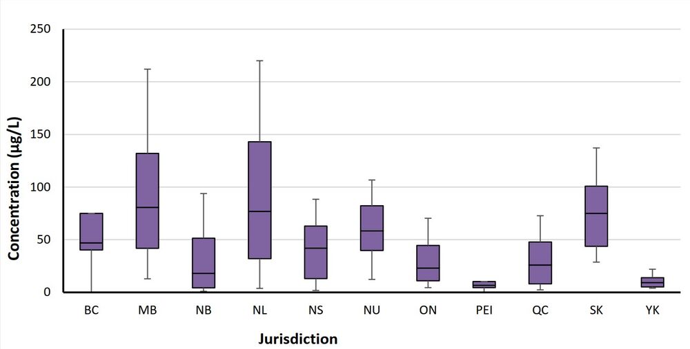
Figure 1 - Text description
The figure describes a chart showing the 10th, 25th, 75th, 90th percentiles and median values of total THM concentrations for each province and territory.
BC = British Columbia, MB = Manitoba, NB = New Brunswick, NL = Newfoundland and Labrador, NS = Nova Scotia, NU = Nunavut, ON = Ontario, PEI = Prince Edward Island, QC = Quebec, SK = Saskatchewan, YK = Yukon
The negative and positive whiskers are equal to the 10th percentile and the 90th percentile concentrations, respectively. The box is equal to the 25th percentile and the 75th percentile concentrations, while the median concentration is presented as a black line in the centre.
| Water source | Parameter | Chloroform (μg/L)Table 3 footnote a |
BDCM (μg/L)Table 3 footnote b |
DBCM (μg/L)Table 3 footnote c |
Bromoform (μg/L)Table 3 footnote cc |
Total THMsTable 3 footnote d (μg/L) |
|---|---|---|---|---|---|---|
| Lake water | # detects/N | 112/112 | 111/112 | 99/112 | 22/112 | 112/112 |
| Detection % | 100.0 | 99.1 | 88.4 | 19.6 | 100.0 | |
| Median | 21.8 | 4.0 | 0.4 | < DL | 28.7 | |
| MeanTable 3 footnote e | 26.6 | 5.9 | 2.0 | 0.2 | 34.6 | |
| 90th percentile | 52.2 | 12.3 | 9.2 | 1.0 | 66.2 | |
| River water | # detects/N | 149/155 | 149/155 | 125/155 | 48/155 | 149/155 |
| Detection % | 96.1 | 96.1 | 80.6 | 31.0 | 96.1 | |
| Median | 18.4 | 3.5 | 0.5 | < DL | 25.3 | |
| MeanTable 3 footnote e | 25.2 | 5.7 | 1.4 | 0.1 | 32.4 | |
| 90th percentile | 51.5 | 14.0 | 5.0 | 5.0 | 63.8 | |
| Well water | # detects/N | 98/108 | 98/108 | 91/108 | 72/108 | 100/108 |
| Detection % | 90.7 | 90.7 | 84.3 | 66.7 | 92.6 | |
| Median | 2.1 | 1.3 | 0.7 | 0.2 | 5.8 | |
| MeanTable 3 footnote e | 4.1 | 2.6 | 2.0 | 0.9 | 9.5 | |
| 90th percentile | 10.9 | 4.5 | 3.8 | 2.0 | 19.3 | |
|
BDCM = bromodichloromethane, DBCM = dibromochloromethane, < DL = less than detection limit (if detection % < 10% then 90th percentile < DL; if detection % < 50% then median < DL), N = sample size; THM = trihalomethanes |
||||||
A study evaluated THM concentrations at the tap in 3 First Nations reserve communities (Amarawansha et al., 2023). All 3 communities use surface water as the source, with conventional treatment and chlorine disinfection. The ranges of THMs were between 96 and 207 μg/L for Community A, 45 and 160 μg/L for Community B, and 57 and 122 μg/L for Community C. Chloroform was the largest contributor to total THM concentration, while brominated THMs (Br-THMs) (BDCM, DBCM and bromoform) comprised less than 5%. There was no significant difference between samples from water piped to homes and those trucked and stored in cisterns.
To compare THM formation in distribution systems from surface water versus groundwater sources, data from different sources were analyzed. These datasets include 2 national surveys and the NDWS (Appendix B: Table B1); and data from Newfoundland and Labrador and Ontario (Appendix B: Table B2). Generally, it was found that:
- Chloroform is higher in surface water
- BDCM had similar levels between ground and surface waters
- DBCM and bromoform levels are slightly higher in groundwater
- Overall, surface water resulted in the formation of higher levels of total THMs
Using the NDWS dataset, data were paired for treated water and a point farthest from the treatment plant (samples taken on same day). These data were then separated for summer and winter (Appendix B: Table B3). It was found that:
- Chloroform and BDCM concentrations were higher for treated and distributed water in summer compared to winter
- There was little change seasonally or between treated and distributed water for DBCM and bromoform
- Total THM concentrations were significantly higher in distributed water than treated water regardless of season, except for bromoform in winter
Similar pairing was done for the Quebec data comparing the centre with an extremity of the distribution system (Appendix B: Table B4) and the Ontario data comparing treated and distributed water (Appendix B: Table B5). For both datasets, there was a significant increase in each THM species with distance in the distribution system, except for bromoform.
Chowdhury et al. (2011) present exposure data for THMs in Canadian provinces, with the data typically spanning 4 to 5 years in the early 2000s. In each province, quarterly samples were taken from an unspecified number to a maximum of 467 drinking water treatment plants. The exact number of samples analyzed was not provided. Generally, this dataset shows similar results to the PT data presented in Figure 1.
Another study evaluated seasonal impacts for 3 water treatment systems (WTSs) in Ontario between 2000 and 2004. Generally, THM concentrations were lower between December and April and higher between June and November (Chowdhury, 2013a).
Water supply systems in Newfoundland and Labrador were studied to evaluate the impacts of source water and treatment plant size based on population served. This study took place over an 18-year period (1999 to 2016) (Chowdhury, 2018). For all systems, regardless of size, those using surface water had higher mean THM concentrations than those using groundwater (Appendix B: Table B6).
Over a 3-year period, 13 systems (with varying treatment) in 6 European countries examined THM concentrations. It was found that higher THM concentrations occurred during summer and fall, with year-to-year variations (Krasner et al., 2016a). Higher THMs occurred in systems using surface water or blended waters than those using groundwater.
The Canadian Health Measures Survey (CHMS) collected tap water samples that were analyzed for THMs in Cycles 3 and 4 (2012 to 2015) (Statistics Canada, 2015, 2017). Each cycle was conducted over 2-year periods from 16 collection site locations across Canada. The study was designed to statistically represent approximately 96% of the Canadian population (Statistics Canada, 2015, 2017). The mean total THM concentration reported was 27.0 μg/L (N = 5,005). This mean is lower than that of many of those calculated from the PT analysis presented in Table 2. This difference is likely due to the purpose of the CHMS study, which was to determine typical THM concentrations in drinking water, without regard for distribution system layout. The PT data presented above are most likely operational or compliance based, with samples collected at points in the distribution system with a high water age with the highest potential THM levels. In addition, the CHMS analyzed samples from only 32 drinking water systems (16 sites per cycle). Although these sites statistically represent 96% of the population, the number of drinking water treatment systems is very small in comparison to the total number of systems across the country, which number in the thousands. The CHMS does not provide details on the drinking water treatment system such as source waters, treatment technologies and distribution system operations. Finally, none of the sites were located in Manitoba, Newfoundland and Labrador (2 of the provinces with the highest mean Total THM levels – see Table 2), Prince Edward Island or any of the territories.
A study evaluating THMs and bromide concentration in the United States showed overall there has not been a significant change in THM concentrations since 1997. However, the extremely high concentrations, represented by 95th percentiles, have been decreasing over time (Westerhoff et al., 2022). At some WTSs, seasonal changes were noted. Generally, these changes were more prevalent in source waters from rivers rather than lakes. Bromide concentrations were found to be higher during periods of lower streamflow. The amount of bromide incorporated into the disinfection by-products to form brominated DBPs was variable with no statistical temporal trends. Groundwater sources tend to have higher Br-THMs.
Limited data exist on I-THM concentrations in Canadian waters. In the National Survey of Disinfection By-Products and Selected Emerging Contaminants, the concentrations of 6 I-THMs were measured in the source water, treated water and distributed water of 65 WTSs across Canada (Health Canada, 2017; Tugulea et al., 2018). The concentrations of these I-THMs in distributed water are presented in Appendix B: Table B7; and for chlorinated and chloraminated systems in Table B8. I-THMs were detected in the distributed water of 48% of WTSs in winter and 71% of WTSs in summer. Total concentrations (sum of all the I-THM congeners measured in one sample) in treated samples ranged from 0.02 μg/L to 21.66 μg/L. The highest total I-THM concentration was measured in a water treatment plant where all 6 I-THMs were detected, with iodoform present at the highest concentration. Maximum concentrations of the detected I-THMs in treated water were 2.27 μg/L for DCIM, 2.91 μg/L for DBIM, 2.06 μg/L for BCIM, 4.31 μg/L for CDIM, 2.71 μg/L for BDIM and 8.3 μg/L for TIM. The highest formation of I-THMs was where source waters had naturally occurring ammonium, high bromide, high iodide and/or total iodine concentrations.
Concentrations of 2 I-THMs were measured in chloraminated and chlorinated drinking waters from 23 cities in Canada and the United States (Richardson et al., 2008). BCIM and DCIM were found at most treatment plants with maximum concentrations of 10.2 μg/L and 7.9 μg/L, respectively. Quebec I-THM data showed that DCIM had the highest concentration (Table B9) (Ministère du Développement durable, de l'Environnement et de la Lutte contre les changements climatiques du Québec, 2019).
Additional water monitoring data were available in the literature for international locations. A study monitoring for 6 I-THMs at 12 drinking water treatment plants in the United States found concentrations of individual I-THMs to range from 0.2 μg/L to 15 μg/L with DCIM being the most frequently detected (Krasner et al., 2006). In a study investigating the trace analysis of emerging DBPs, concentrations of BCIM ranged from below the detection limit to 0.120 μg/L at 4 water treatment plants in the United States. (Cuthbertson et al., 2020).
In a study of 70 drinking water treatment plants in 31 cities across China, concentrations of DCIM and BCIM ranged from below the detection limit to 3.67 μg/L for DCIM and below the detection limit to 1.91 μg/L for BCIM. DBIM and TIM were not detected in any of the samples (Ding et al., 2013). The presence of 6 I-THMs was investigated in a drinking water supply network in Spain. Concentrations ranged between 0.18 and 0.31 μg/L, with DCIM detected at the highest levels (Postigo et al., 2018). In a study of household tap water in 2 cities in Cyprus (n = 37), DCIM was the dominant species of the 2 measured I-THMs with concentrations ranging between 0.032 μg/L and 1.65 μg/L. BCIM was also detected at concentrations below the limit of detection to 0.45 μg/L (Ioannou et al., 2016).
1.3.2 Multi-route exposure through drinking water
Due to their physicochemical properties, THMs are highly volatile and are permeable through the skin. As a consequence, the inhalation and dermal absorption of THMs during bathing or showering are important routes of exposure (Jo et al., 1990a,b, 2005; Weisel and Jo, 1996; Backer et al., 2000; Xu et al., 2002; Xu and Weisel, 2005). Various exposure assessments have estimated the relative contribution of the ingestion, inhalation and dermal exposure routes to the total daily intake of THMs. The results of these assessments are mixed with several studies suggesting that the inhalation of THMs may result in exposures that are equal to or larger than exposures due to ingestion of drinking water (Krishnan, 2003; Kim et al., 2004; Jo et al., 2005; Basu et al., 2011; Pardakhti et al., 2011; Zhang et al., 2018a; Genisoglu et al., 2019). Another study suggests that inhalation and dermal exposures are comparable, but less than ingestion (Chowdhury, 2013b), while another study suggests that inhalation and dermal exposures are greater than ingestion (Yanagibashi et al., 2010). Still other studies suggest that dermal absorption can contribute more heavily to internal dose than inhalation and ingestion, specifically in the case of BDCM (Krishnan, 2003; Leavens et al., 2007; Kenyon et al., 2016). Factors that may influence the rates of uptake via the various routes include water temperature, duration of exposure and air exchange rates, among others.
Studies have derived modifying factors (litre-equivalents per day [Leq/day]) to quantify the amount of THMs that people are exposed to via the different exposure routes (that is, dermal and inhalation), especially during showering and bathing. Krishnan (2003) determined Leq/day values for exposures of adults and children (6-, 10- and 14-year-olds) during a 10-minute shower and 30-minute bath with tap water. The Leq/day values were calculated using physiologically based pharmacokinetic modelling (PBPK) model-generated data on the absorbed fraction (Corley et al., 1990, 2000; Price et al., 2003; Haddad et al., 2006). Calculations accounted for inter-chemical differences in the water-to-air factor (based on differences in Henry's law constants), fraction of dose absorbed during inhalation and dermal exposures, and skin permeability coefficient. The absorbed fraction for the dermal and inhalation exposures took into consideration the dose that was absorbed following exposure as well as that portion that was exhaled in the following 24 hours. Complete (100%) absorption of ingested THMs was assumed for all subpopulations; this was supported by the available information on the hepatic extraction of the THMs (Da Silva et al., 1999; Corley et al., 2000).
Leq/day values were highest for the adult sub-group for both bath and shower exposure scenarios. In addition, Leq/day values for the inhalation and dermal routes were higher for the 30-minute bath scenario than for the 10-minute shower for all subpopulations based on the longer exposure time. The bath scenario values were considered to be conservative, since most Canadians do not take a 30-minute bath daily (Table 4). In addition, in the event that individuals are exposed to THMs via other household activities or additional bathroom time, the Leq/day values calculated for the bath scenario are protective of these additional exposures. The Leq/day values calculated by Krishnan (2003) were used in the derivation of the HBVs for THMs (see section 3.0, Derivation of the health-based value).
| THM | Oral (L/day) |
Inhalation (Leq/day) | Dermal (Leq/day) | Total (Leq/day) |
|---|---|---|---|---|
| Chloroform | 1.5 | 1.70 | 0.91 | 4.11 |
| BDCM | 1.5 | 0.67 | 1.38 | 3.55 |
| DBCM | 1.5 | 0.50 | 1.60 | 3.60 |
| Bromoform | 1.5 | 0.46 | 1.78 | 3.74 |
|
BDCM = bromodichloromethane, DBCM = dibromochloromethane |
||||
1.3.3 Swimming pools and hot tubs
Dermal and inhalation exposure to THMs may occur in swimming pools and hot tubs where chlorine, which is used as a disinfectant, reacts with organic matter (for example, sweat, hair, lotion) present in the water. Several studies have examined levels of THMs in plasma, urine, and the breath of swimmers and pool workers (Levesque et al., 1994; Lindstrom et al., 1997; Aggazzotti et al., 1998; Whitaker et al., 2003; Erdinger et al., 2004; Caro and Gallego, 2008; Marco et al., 2015; Font-Ribera et al., 2016). In general, bodily concentrations of THMs were observed to increase with the time spent swimming and the level of exertion. Limited information suggests that users of hot tubs may have more significant dermal uptake than swimmers due to higher water temperatures (Wilson, 1995).
1.3.4 Biomonitoring data
Chloroform, BDCM, DBCM and bromoform were analyzed in the whole blood of participants aged 12 to 79 in CHMS cycle 3 (2012 to 2013), cycle 4 (2014 to 2015) and cycle 5 (2016 to 2017) (Health Canada, 2019a). Blood concentrations for BDCM, DBCM and bromoform were largely below the detection limits for all 3 of the survey cycles for all age groups. Mean blood concentrations of chloroform were not calculated for cycles 3 and 4 as more than 40% of samples were below the detection limit of 0.014 µg/L. However, in cycle 5 a lower detection limit was established (0.006 µg/L), and the mean blood concentration of chloroform in participants aged 12 to 79 was 0.011 µg/L. These blood concentrations were below the biomonitoring equivalent level of 0.230 µg/L derived from the United States Environmental Protection Agency's (U.S. EPA) oral reference dose of 0.01 mg/kg body weight (bw) per day (Aylward et al., 2008).
Although an analytical method was developed to detect and quantify 2 I-THMs (DCIM and BCIM) in whole blood (method detection limit = 2 ng/L), no biomonitoring data were located for I-THMs (Silva et al., 2006).
2.0 Health considerations
2.1 Kinetics
Although kinetic information is available for chloroform and the brominated THMs, no data are available regarding the absorption, distribution, metabolism, excretion and PBPK modelling of I-THMs.
2.1.1 Absorption
2.1.1.1 Chloroform
Chloroform is readily absorbed via all routes of exposure. Following oral exposure, the gastrointestinal absorption of chloroform is upwards of 90% depending on the delivery vehicle; more rapid absorption occurs with an aqueous solution as opposed to oil (Withey et al., 1983). Chloroform absorption in the lung is considerable with chloroform readily passing from air to blood in the human alveoli (Corley et al., 1990; Batterman et al., 2002). Several animal and human studies have demonstrated that chloroform can be absorbed through intact skin, including from water while showering and bathing. Dermal absorption rates in human volunteers range from 1.6% to 7.8% depending on the delivery vehicle (Jo et al., 1990b; Bogen et al., 1992; Dick et al., 1995).
2.1.1.2 Brominated THMs
Brominated THMs are well absorbed following oral exposure with absorption rates in animal studies ranging between 60% and 90% (Mink et al., 1986; Mathews et al.,1990). Absorption rates vary based on the administration vehicle with greater absorption observed for aqueous vehicles (ATSDR, 2020). Although data are limited, based on physical-chemical properties, it is expected that the brominated THMs would be well absorbed by the lung (ATSDR, 2005). However, this absorption may be to a lesser extent than for chloroform (Yoshida et al., 1999). Brominated THMs are readily absorbed through the skin (ATSDR, 2005; ATSDR, 2020). An in vitro study using human skin found brominated THMs to be more absorbed than chloroform, with bromoform being the most permeable through the skin (Xu et al., 2002).
2.1.2 Distribution
2.1.2.1 Chloroform
Chloroform is distributed throughout the body but tends to accumulate in lipid-rich tissues. The highest levels have been found in the fat, liver, kidneys, nervous system, lungs and blood (ATSDR, 1997). Distribution is dependent on exposure route; extrahepatic tissues receive a higher dose from inhaled or dermally absorbed chloroform than from ingested chloroform. Placental transfer of chloroform has been demonstrated in several animal species and humans. Unmetabolized chloroform is retained longer in fat than in any other tissue (WHO, 2005).
2.1.2.2 Brominated THMs
2.1.3 Metabolism
2.1.3.1 Chloroform
The toxicity of chloroform is attributable to its metabolites. Oxidative and reductive pathways for chloroform metabolism have been identified, both of which proceed through a cytochrome P450 (CYP2E1)-dependent bioactivation step. The balance between oxidative and reductive pathways depends on species, tissue, dose and oxygen tension. Of the tissues with chloroform-metabolizing ability, the liver is the most active, followed by the nose and kidney (Environment Canada and Health Canada, 2001).
At the low levels typical of actual human exposure to chloroform in drinking water, the majority of chloroform is metabolized oxidatively via CYP2E1 to produce trichloromethanol (Gemma et al., 2003). Trichloromethanol has an extremely short half-life and spontaneously decomposes to produce phosgene, a highly reactive electrophilic compound. Phosgene may then be detoxified by reaction with water to produce carbon dioxide (major metabolite) and hydrochloric acid. Alternatively, phosgene can form covalent bonds with the nucleophilic components of tissue proteins, as well as with other cellular nucleophiles, or bind to the polar heads of phospholipids; little binding of chloroform metabolites to deoxyribonucleic acid (DNA) has been observed. Phosgene can also undergo glutathione-dependent reduction to oxidized glutathione and carbon monoxide. Both phosgene and hydrochloric acid can cause tissue damage and the reaction of phosgene with tissue proteins is associated with cell damage and death (Environment Canada and Health Canada, 2001).
In addition to oxidative biotransformation, chloroform can undergo reductive dehalogenation to produce the dichloromethyl radical. These reactive radicals may bind covalently to a variety of cellular macromolecules. This reductive pathway is not as relevant in the human liver since it is active only at high substrate concentrations, and in strictly anaerobic conditions.
The metabolism of chloroform varies with sex and species. Mice have been observed to metabolize chloroform faster than rats and, due to renal CYP2E1 levels increased by testosterone, male mice are more sensitive than female mice to chloroform-induced renal toxicity (Sasso et al., 2013).
2.1.3.2 Brominated THMs
Like chloroform, brominated THMs are metabolized through both oxidative and reductive pathways. Approximately 70% to 80% of BDCM is metabolized by CYP2E1 to carbon dioxide via phosgene (Lilly et al., 1997; Allis et al., 2002), while DBCM and bromoform are metabolized via brominated analogues of phosgene.
In addition, brominated THMs can be metabolized through a third pathway: glutathione S-transferase theta-mediated conjugations. Unlike chloroform, brominated THMs undergo transformation by glutathione transferase theta 1-1 (GSTT1-1) to mutagenic intermediates at low substrate concentrations (Pegram et al., 1997; Ross and Pegram, 2003). Although this pathway is quantitatively minor compared with oxidation and reduction (based on catalytic efficiency), the mutagenic metabolites that are formed may result in a disproportionately toxic response (ATSDR, 2005, 2020).
The International Programme on Chemical Safety (IPCS, 2000) postulated that brominated THMs may be more rapidly and more extensively metabolized than their chlorinated counterparts. Although this may be true for BDCM, support for this statement as it pertains to DBCM or bromoform is difficult to determine from the limited literature currently available.
In a study with chloroform, BDCM, DBCM and bromoform, Mink et al. (1986) found clear interspecies differences in the metabolism of THMs, with metabolism in mice being 4- to 9-fold greater than that in rats. However, note that the administered doses were high and that metabolism in both species is more complete following administration of lower, more relevant doses.
In humans, inter-individual variation in the CYP2E1 and glutathione S-transferase (GST) family enzymes involved in the metabolism of THMs may affect sensitivity to the toxic effects of THMs (OEHHA, 2020).
2.1.3.3 Mixtures of THMs
A PBPK model was developed by Da Silva et al. (2000), who found that exposures to binary mixtures of chloroform and BDCM, DBCM or bromoform would likely result in significant increases in the levels of unmetabolized chloroform in the blood, relative to chloroform administered alone. This study also demonstrated that clearance of THMs may be impacted by toxicokinetic interactions between THMs. Bromoform and DBCM appear to persist in blood and tissues for longer periods of time when co-administered with chloroform than when given alone (GlobalTox, 2002).
2.1.4 Excretion
2.1.4.1 Chloroform
Chloroform is rapidly and primarily eliminated through expired air as carbon dioxide and unchanged chloroform. In animals, the fraction eliminated as carbon dioxide varies with the dose and the species (IPCS, 2000). In human studies, there is substantial inter-individual variability in the fraction of the dose eliminated as carbon dioxide. Peak chloroform and carbon dioxide concentrations were detected in the expired breath 40 minutes and 2 hours respectively after administration of a single oral dose of chloroform in olive oil. An inverse relationship between the adipose tissue content of the body and pulmonary elimination of chloroform was noted (Fry et al., 1972).
2.1.4.2 Brominated THMs
As with chloroform, the major route of excretion for brominated THMs is through expired air, primarily as the parent compound or as carbon dioxide; smaller amounts are excreted through the urine and feces (Mink et al., 1986; Mathews et al., 1990). Lilly et al. (1998) found that in animals, more of the parent BDCM compound was eliminated unmetabolized via exhaled breath after aqueous dosing than after corn oil gavage. The half-lives of THMs following a single oral dose in rats were 0.8 hours for bromoform, 1.2 hours for DBCM, 1.5 hours for BDCM and 2 hours for chloroform. In mice, the half-lives were 8 hours for bromoform, 2.5 hours for DBCM and BDCM, and 2 hours for chloroform (Mink et al., 1986). The half-life for BDCM in monkeys was 4 to 8 hours (Smith et al., 1985). Elimination kinetics have also been studied and modelled in humans swimming in chlorinated pools (Lindstrom et al., 1997; Pleil and Lindstrom, 1997). Half-lives of 53 minutes for chloroform and 23 minutes for BDCM, as measured in the urine, were observed, with the absorbed dose being eliminated after 2 hours (Caro and Gallego, 2007). In a study of volunteers during a controlled showering exposure, bromoform levels in the blood were the slowest of the 4 THMs to decrease after a 10-minute shower, likely due to the greater lipophilicity of bromoform and higher retention in adipose tissue (Silva et al., 2013).
2.1.5 Physiologically based pharmacokinetic modelling
Physiologically based pharmacokinetic modelling (PBPK) models describe the rate of absorption, distribution, metabolism and elimination of xenobiotics in humans and experimental animals. PBPK modelling can provide useful information to extrapolate between and within species and can be used to refine the uncertainty factors applied in a risk assessment.
2.1.5.1 Chloroform
A number of PBPK models have been created to describe the toxicokinetics of chloroform via oral and/or inhalation exposures (Feingold and Holaday, 1977; Corley et al., 1990; Gearhart et al., 1993; ICF Kaiser, 1999; Sasso et al., 2013). A further number of models have added a dermal absorption component to the PBPK models (Chinery and Gleason, 1993; McKone, 1993; Corley et al., 2000; Haddad et al., 2006; Tan et al., 2006). Many of these models were based on the PBPK model by Corley et al. (1990). The first extensive model for chloroform, it is a 5-compartment model which describes the toxicokinetics of chloroform in rats, mice and humans via the oral and inhalation routes of exposure and identifies the kidney and liver as the primary sites for metabolism. More recently, Sasso et al. (2013) built upon the model of Corley et al. (1990) and provided improved estimates of renal chloroform metabolism by accounting for regional differences in the kidney's metabolic capacity. The model established new rate parameters for chloroform metabolism in rats, mice and humans. For model validation, the model was tested using assumptions identical to those in the Corley PBPK model and was able to reproduce the original results for simulations of data for chloroform uptake, exhalation and tissue deposition from inhalation data in rodents, drinking water data in humans and oral gavage data in rodents. The model provided adequate fits to the data and predictions remained within 2-fold of the data. The Sasso model was also compared with newer data provided by the Japan Bioassay Research Center (Take et al., 2010). Chloroform concentrations measured in kidney, liver, blood and adipose tissue in male rats were consistent with the PBPK model predictions for all exposure pathways (that is, oral, inhalation and combined oral/inhalation). Using the PBPK model, the authors found that the kidney dose metric was highly influenced by the oral exposure profile (that is, continuous daily dose over 24 hours at low levels versus bolus events occurring a few times a day). Therefore, since actual water ingestion patterns are better represented by exposure through multiple discrete events, the water consumption model by Spiteri (1982) was applied in the PBPK simulations. The PBPK model by Sasso et al. (2013) was used in the current assessment of chloroform to convert administered doses in rodents to internal doses and then to estimate human-equivalent doses.
2.1.5.2 Brominated THMs
Lilly et al. (1997) developed a 5-compartment model to estimate the rates of BDCM metabolism in rats via inhalation. A subsequent model linked a multi-compartment gastrointestinal tract sub-model to the PBPK model to describe the tissue dosimetry and metabolism of orally ingested BDCM in rats (Lilly et al., 1998). The National Toxicology Program (NTP) (2006) developed a PBPK model based on improvements to the Lilly et al. (1998) model, which included a description of tissue-specific metabolism via the GST pathway, inclusion of metabolic activity in the large intestine, distribution of BDCM to organs that is diffusion-limited rather than flow-limited, non-linear behaviour in the oral absorption of BDCM, description of the rates of transit through the different compartments of the gastrointestinal tract and a description of the rodents' drinking water pattern during the assay. The current assessment uses the NTP (2006) PBPK model of BDCM to convert administered doses to internal doses to facilitate the comparison of data between studies.
2.2 Effects in humans
A large number of epidemiological studies have examined the association between human exposure to THMs in drinking water and a range of adverse outcomes. The analyses of these relationships are complicated since exposure to THMs in drinking water involves co-exposure to other DBPs. With upwards of 600 DBPs identified in drinking water, it is a challenge to identify the drivers of health effects or to assign causation to any single component (Richardson et al., 2007). Despite these challenges, the preponderance of epidemiological studies has focused on evaluating cancer and reproductive and developmental outcomes in relation to THM exposure. No epidemiological studies investigating associations with exposure to I-THMs have been identified.
2.2.1 Cancer epidemiology
Bladder cancer is the most studied outcome with regards to THMs and cancer. More than a dozen case-control, cohort and ecological studies support an association between exposure to THMs, used as a surrogate for DBPs in drinking water, and cancer of the bladder (see OEHHA, 2020, for a review of epidemiological studies; see also Evlampidou et al., 2020). Similarly, the International Agency for Research on Cancer (IARC) review of DBPs in chlorinated drinking water identifies consistent associations between THMs and bladder cancer (IARC, 2013).
A meta-analysis performed on 6 case-control studies and 2 cohort studies from North America and Europe evaluated bladder cancer in relation to consumption of chlorinated drinking water (but not specifically THMs in drinking water). The consumption of chlorinated drinking water was associated with an increased risk of bladder cancer in men (combined odds ratio [OR] = 1.4; 95% confidence interval [CI] = 1.1 to 1.9) and women (combined OR = 1.2; CI = 0.7 to 1.8) (Villanueva et al., 2003).
A pooled analysis of the primary data from 6 case-control studies in North America and Europe evaluated bladder cancer over a common 40-year window of exposure to THMs. The results showed increasing relative risks with increasing exposure among men, with an OR of 1.44 (CI = 1.20 to 1.73) for exposure higher than 50 μg/L. THM exposure was not associated with bladder cancer risk in women (OR = 0.95; CI = 0.76 to 1.20) (Villanueva et al., 2004). A subsequent meta-analysis including some of the same case-control studies as Villanueva et al. (2004) as well as some additional studies revealed a significant exposure-risk association between THMs and bladder cancer (linear trend p = 0.01). Further, men exposed to >50 μg/L had a significantly increased OR (OR = 1.47; CI = 1.05 to 2.05) compared with men exposed to levels less than 5 μg/L (Costet et al., 2011).
The scientific evidence concerning the association of chlorinated DBPs and human bladder cancer was evaluated by an interdisciplinary panel commissioned by the Water Research Foundation and the American Water Works Association (Hrudey et al., 2015). This review concluded that the majority of case-control studies suggest an association of bladder cancer with exposure to chlorinated DBPs (although there is no evidence of causation), published meta-analyses support an association between chlorinated DBPs and bladder cancer, and brominated DBPs may be more important than chlorinated DBPs with regards to an association with bladder cancer. It has been postulated that the brominated THMs in drinking water may play a causative role in the development of bladder cancer.
Mechanistic studies in bacterial models show that brominated THMs are metabolically activated to mutagenic compounds by the glutathione S-transferase theta-1 (GSTT1) enzyme (DeMarini et al., 1997; Pegram et al., 1997). GSTT1 is active in the urinary tract and studies have shown that GSTT1-mediated metabolism of BDCM produces reactive intermediates that covalently bind to DNA (that is, BDCM is a potential mutagenic carcinogen) (Ross and Pegram, 2003, 2004). GSTT1 polymorphisms have been identified in humans and it has been found that people who express this enzyme have a greater risk (OR = 1.8; CI = 1.1 to 3.1) for developing bladder cancer when exposed to upper quartile concentrations (> 49 μg/L) compared with those who are GSTT1-null (Cantor et al., 2010).
In contrast to other findings, a recent analysis examined the incidence of bladder cancer in 8 countries in the 45 years since THMs were detected in chlorinated drinking water. It concluded that bladder cancer risk from drinking water remains questionable largely because of the imprecise THM exposure estimates that are generally used in epidemiological studies. The review states that bladder cancer risks from drinking water and THMs are likely small and overwhelmed by other risk factors, such as smoking, diabetes and other country-specific aspects (Cotruvo and Amato, 2019). This analysis was based on a broad assessment of national average THM concentrations and national bladder cancer rates in the United States. It did not consider individual studies that evaluate the specific THM concentrations to which people with bladder cancer were exposed.
Additional epidemiological studies have investigated the incidence of other types of cancer in relation to THMs in drinking water. These include colorectal, brain, pancreatic, esophageal, lung, kidney, stomach, lympho-hematopoietic, ovarian, prostate and breast cancer (see OEHHA 2020 for a review). Although some of these studies have identified associations with THMs in drinking water, the data appear to be less consistent than the associations with bladder cancer and are inconclusive.
Overall, the epidemiological evidence points to an association between exposure to THMs in drinking water and bladder cancer. However, the epidemiological studies have several limitations that prevent their use in the quantitative risk assessment. These include imprecise exposure estimates (for example, using regional THM water concentrations instead of individual exposure data, not using integrated bathing and oral consumption exposures, intra- and inter-individual variability in water use patterns) as well as more general limitations such as study size, confounding and other forms of bias. More importantly, however, is the fact that numerous DBPs are present in drinking water and therefore risk cannot be attributed exclusively to THMs.
2.2.2 Reproductive and developmental epidemiology
A substantial number of studies have investigated possible associations between exposure to THMs in drinking water and adverse reproductive and developmental outcomes. Various endpoints have been examined, including stillbirths, spontaneous abortion (miscarriage), preterm or premature birth, low birth weight, small for gestational age (SGA) and birth defects/congenital anomalies (which consist of a highly heterogeneous group of outcomes [for example, cardiac, urinary, respiratory, nervous system, oral cleft defects]). Most studies have focused on developmental risks or female reproductive outcomes. In contrast, very few studies focusing on male reproductive endpoints (for example, sperm quality) have been undertaken (for example, Luben et al., 2007; Iszatt et al., 2013; Zeng et al., 2016; Chen et al., 2020; Wei et al., 2022; Liu et al., 2023).
In 2008, Health Canada convened an expert panel to review the reproductive and developmental toxicity associated specifically with BDCM. The expert panel concluded that "Overall, the evidence from epidemiological studies is inconsistent and by international standards, the current weight of evidence is not sufficient to support an association between adverse reproductive and developmental effects in humans and environmental exposures to BDCM" (Health Canada, 2008a).
Since then, several pooled analyses and meta-analyses have investigated the relationship between long-term exposures to THMs and reproductive and developmental outcomes. One review and meta-analysis of 15 case-control and cross-sectional population-based studies from North America, Europe and Taiwan evaluated exposure to chlorinated DBPs and congenital anomalies. The individual studies reviewed showed inconsistent results for an association between DBPs and risk of all congenital anomalies combined as well as for specific groups of anomalies. The meta-analysis revealed a statistically significant excess risk for high versus low exposure to chlorinated water or THMs and all congenital anomalies combined (17%; CI = 3 to 34), based on a small number of studies. The meta-analysis also suggested a statistically significant excess risk for ventricular septal defects (58%; CI = 21 to 107), but this was based on only 3 studies, and there was little evidence of an exposure–response relationship (Nieuwenhuijsen et al., 2009). A subsequent individual study examining craniofacial birth defects found elevated adjusted odds ratios for cleft palates and THMs as well as eye defects and chloroform, although no exposure-response patterns were discernable (Kaufman et al. 2018).
Another meta-analysis of 15 population case-control studies, retrospective pregnancy cohort studies or prospective pregnancy cohort studies evaluated associations between exposure to THMs in drinking water and indicators of fetal growth and prematurity. The analysis found little or no evidence for associations with most indicators of fetal growth and preterm birth, with the possible exception of SGA. The risks of SGA for third trimester exposure to 80 μg/L and 100 μg/L of THMs were OR = 1.08 (CI = 1.01 to 1.17) and 1.10 (CI = 1.01 to 1.21), respectively (Grellier et al., 2010).
Another study systematically reviewed the evidence on the risks of miscarriage, preterm or premature birth, low birth weight and SGA associated with exposure to THMs. Nine of the 29 studies reviewed showed evidence of an association between maternal THM exposure and adverse pregnancy outcomes (Dodds et al., 1999; Aggazzotti et al., 2004; MacLehose et al., 2008; Grazuleviciene et al., 2011; Levallois et al., 2012; Rivera-Núñez and Wright, 2013; Iszatt et al., 2014; Kumar et al., 2014; Cao et al., 2016). Twenty studies reported no association with adverse pregnancy outcomes. Overall, maternal exposure to THMs was associated with SGA and a slightly increased risk of miscarriage (Mashau et al., 2018). A further individual study found increased adjusted odds ratios for stillbirth and exposure to chloroform and BDCM (Rivera-Núñez et al., 2018).
Another systematic review looked specifically at the impact of chloroform on reproductive and developmental outcomes. Of the 42 studies examined, most (30) of the studies focused on developmental outcomes, with the remainder focusing on male and female reproductive outcomes. The weight of evidence examined in this review did not support an association between chloroform exposure during pregnancy and risk of birth defects, postnatal weight gain or SGA. In addition, the evidence showed a potential protective association between chloroform exposure and preterm birth, possibly due to a confounding effect (for example, higher socioeconomic status and healthier lifestyle) (Williams et al., 2018).
A large nationwide prospective cohort study was conducted in Sweden between 2005 and 2015 to assess the association between total THMs in drinking water and the risk of SGA, preterm delivery and congenital malformations. Based on approximately 500,000 births, a significant increase in SGA was observed in the highest THM exposure group (total THMs > 15 μg) in areas with hypochlorite treatment compared with the unexposed group (OR = 1.20; CI = 1.08, 1.33). No clear associations were observed between THMs and preterm delivery (Säve-Söderbergh et al., 2020). Based on over 620,000 births, associations were observed between the highest total THM exposure groups in areas using chloramine and malformations of the nervous system (OR = 1.82; CI = 1.07, 3.12), urinary system (OR = 2.06; CI = 1.53, 2.78), genitals (OR = 1.77; CI = 1.38, 2.26), and limbs (OR = 1.34; CI = 1.10, 1.64) (Säve-Söderbergh et al., 2021).
Despite the existence of some well-conducted studies with large sample sizes, improved personal exposure assessment and consideration of multiple exposure pathways, the conclusions of individual studies vary, with some studies suggesting adverse associations with THMs, and others indicating no association. Among the reviews and meta-analyses, there appears to be some indication of a potential association with SGA. However, the epidemiological evidence is insufficient to determine whether any observed associations are causal. In addition, with numerous DBPs present in drinking water, it is impossible to attribute any risk exclusively to THMs.
2.3 Effects in animals
Exposure to THMs is well known to result in a number of adverse effects in animal models. The liver and kidney appear to be the primary target organs for adverse effects, although depending on the THM, effects are also observed in other organs and tissues, including the colon, thyroid and nasal tissues. Although reproductive and developmental effects have also been observed in animal studies, these effects were inconsistent among animal models and largely occurred at high doses that also caused maternal toxicity.
2.3.1 Effect of vehicle and delivery method
In laboratory studies, animals are dosed with concentrations of THMs that are substantially higher than those typically found in drinking water. At these higher levels, THMs are often insoluble in drinking water and are too volatile to administer through the diet in feed (NTP, 1985). Consequently, many laboratory studies administer THMs through gavage in corn oil to ensure the animals are properly dosed. However, delivery of THMs via gavage in corn oil has often resulted in effects not observed when the chemicals are administered through drinking water. This may be due to a number of factors.
When THMs are delivered in drinking water, they are consumed incrementally as opposed to in a bolus dose as occurs when THMs are delivered via gavage. Animals given THMs in drinking water often initially consume less water than controls, likely because of the decreased palatability of the dosed water. However, even when water and THM consumption increases with time, reduced toxicity has been observed as compared to gavage, indicating a tolerance to toxic effects (Coffin et al., 2000). This may be a result of lower concentrations in the liver and consequently a greater opportunity for metabolism without overwhelming detoxification mechanisms.
The use of oil as a vehicle adds to the caloric intake of the animal, and can also change the toxicokinetics (for example, the absorption) of the test material (Hayes and Kruger, 2014). Furthermore, corn oil is known to act as a tumour promoter (Wu et al., 2004). These factors can cause differences in toxicity, particularly in longer-term studies.
In addition, corn oil administered as a vehicle has been found to cause changes in the intestinal microbiome, mRNA expression of intestinal permeability and immune response-related genes in CD-1 mice but not Sprague Dawley rats (Gokulan et al., 2021). The implication of these findings for chemical toxicity assessment is unknown.
The ramifications of using corn oil gavage as compared to drinking water in exposure studies are difficult to discern and may vary according to other study parameters (for example, length of study, endpoint investigated, dietary factors). This may explain why some comparative studies have observed adverse effects following delivery of THMs (particularly chloroform) in corn oil but not drinking water (Bull et al., 1986; Larson et al., 1995a; Pereira and Grothaus, 1997), while other studies have observed similar adverse effects following both corn oil and water exposure (Geter et al., 2004a).
2.3.2 Acute/subchronic/chronic toxicity
2.3.2.1 Chloroform
The animal toxicity database for chloroform covers inhalation and oral exposure (that is, drinking water, gavage) and addresses several endpoints in rats, mice, guinea pigs, rabbits and dogs (see ATSDR [1997] and OEHHA [2020] for more thorough reviews). The liver and kidney appear to be the primary target organs, although there is evidence for nasal lesions as well.
Acute oral exposures of rats and mice to chloroform resulted in a wide range of median level dose (LD50) values ranging from 36 to 2,180 mg/kg, due in part to strain variability and age of dosing (OEHHA, 2020). High acute exposures have resulted in central nervous system and respiratory depression, cardiac arrhythmia, and liver and kidney damage. Short duration studies in rats and mice have identified the liver and kidney as critical target organs (Condie et al., 1983; Plummer et al., 1990; Larson et al., 1994a, b, 1995a, b; Melnick et al., 1998).
A number of subchronic studies have investigated the exposure of animals to chloroform via oral ingestion or inhalation. These studies are presented in Table 5 and Table 6, respectively. Included in these tables are studies that investigated multiple doses and that had exposure durations of 90 days or more. Effects in the liver and kidney were observed at doses as low as 50 mg/kg per day for oral studies and 30 ppm for inhalation studies. Nasal effects were observed at doses as low as 2 ppm. Variation in species sensitivity has been reported in animals exposed to chloroform via inhalation with hepatic and renal lesions in mice being the most sensitive (Torkelson et al., 1976; Sasso et al., 2013).
| NOAEL/LOAEL (mg/kg bw per day) | Species, sex, number | Dose and route | Exposure duration | Critical effect(s) | Reference |
|---|---|---|---|---|---|
| 150Table 5 footnote a/410 | Rat, SPF Sprague-Dawley, M, F, 10/sex/dose | 0, 15, 30, 150, 410 mg/kg bw per day, gavage (toothpaste) | 13 weeks | Increased liver weight with fatty change and necrosis | Palmer et al. (1979) |
| 45/150 (M) 45/142 (F) |
Rat, Sprague-Dawley, M, F, 20/sex/dos | 5, 50, 500 or 2,500 mg/LTable 5 footnote b, drinking water | 90 days (plus 90 recovery days) | Decreased food intake and increased mortality | Chu et al. (1982) |
| NA/50 (F) 125/250 (M) |
Mice, CD-1, M, F, 7-12/sex/dose | 0, 50, 125, 250 mg/kg bw per day, gavage (Emulphor water) | 90 days | Increased liver weight and decreased hepatic microsomal activity, microscopic tissue changes in the liver and kidney | Munson et al. (1982) |
| NA/60 | Mice, B6C3F1, M, F, 10/sex/dose | 60, 130, 270 mg/kg bw per day, gavage (corn oil or 2% Emulphor) | 90 days | Increased liver weight (corn oil and Emulphor delivery). Increased SGOT, decreased TG, vacuolation and lipid accumulation in the liver (corn oil delivery only) | Bull et al. (1986) |
|
F = females; LOAEL = lowest-observed-adverse-effect level, M = males, NA = The study did not have a NOAEL or LOAEL, NOAEL = no-observed-adverse-effect level, SGOT = serum glutamate oxalacetate transaminase, TG = triglyceride |
|||||
| Species, sex | Dose | Exposure duration | Critical effect(s) | Reference |
|---|---|---|---|---|
| Rats, rabbits, guinea pigs, dogs, M, F | 25, 50, 85 ppmTable 6 footnote a | 7 hrs/day, 5 days/week for 6 months | Liver and kidney toxicity ≥ 25 ppm. Rats were the most sensitive and guinea pigs were the least | Torkelson et al. (1976) |
| Mouse, B6C3F1, M, F | 0, 0.3, 2 10, 30, 90 ppmTable 6 footnote b | 6 hrs/day, 7 days/week, 13 weeks | Hepatic lesions ≥ 30 ppm, renal lesions ≥ 30 ppm, nasal effects ≥ 10 ppm | Larson et al. (1996) |
| Rat, F344/N, M, F | 0, 2 10, 30, 90, 300 ppmTable 6 footnote c | 6 hrs/day, 7 days/week, 13 weeks | Hepatic lesions at 300 ppm, renal lesions ≥ 30 ppm, nasal effects ≥ 2 ppm | Templin et al. (1996) |
| Mouse, BDF1, M, F | 0, 1, 5, 30, 90 ppmTable 6 footnote d | 6 hrs/day, 5 days/week, 13 weeks | Hepatic vacuolation and degeneration at 90 ppm, kidney effects ≥ 30 ppm | Templin et al. (1998) |
| Rat, F344, M, F | 25, 50, 100, 200 or 400 ppmTable 6 footnote e |
6 hrs/day, 5 days/week, 13 weeks | Nasal effects ≥ 25 ppm, liver and kidney effects ≥ 100 ppm | Kasai et al. (2002) |
| Mouse, BDF1, M, F | 12, 25, 50, 100 or 200 ppmTable 6 footnote f | 6 hrs/day, 5 days/week, 13 weeks | Kidney and nasal effects ≥ 12 ppm, liver effects 100 ppm | Kasai et al. (2002) |
|
F = females, M = males. |
||||
Effects in the liver and kidney have also been observed in chronic studies of rats, mice and dogs exposed to chloroform (Table 7). One study in particular examined the effects of combined exposure to chloroform via inhalation and drinking water (Nagano et al., 2006). Since most chronic studies are designed as cancer bioassays, further details on these and other studies are available in section 2.3.4.1, Genotoxicity and carcinogenicity.
| NOAEL/ LOAEL (mg/kg bw per day) | Species, sex, number | Dose and route | Exposure duration | Critical effects(s) | Reference |
|---|---|---|---|---|---|
| 64/129 (M) 71/143 (F) |
Rat, Osborne- Medel, M, F, 50/sex/dose | 0, 90, 180 mg/kg (M); 0, 100, 200 mg/kg (F)Table 7 footnote a, gavage (corn oil) | 78 weeks (5 days/week) | Hepatic necrosis, urinary bladder hyperplasia, splenic hematopoiesis, decreased body weight gain and survival, testicular atrophy | NCI (1976) and re-evaluation of data by Reuber (1979) |
| NA/99 (M) NA/170 (F) |
Mouse, B6C3F1, M, F, 50/sex/dose | 0, 138, 277 mg/kg (M); 0, 238, 477 mg/kg (F)Table 7 footnote b, gavage (corn oil) | 78 weeks (5 days/week) | Hepatic hyperplasia, some hepatic necrosis and (in females only) heart thrombosis | NCI (1976) and re-evaluation of data by Reuber (1979) |
| NA/13 | Dog, Beagle, M, F, 8/sex/dose | 0, 15, 30Table 7 footnote c mg/kg gavage (toothpaste base in gelatin capsule) | 7.5 years (6 days/week) | Increased SGPT and fatty cysts in the liver | Heywood et al. (1979) |
| 38/81 | Rat, Osborne Mendel, M, 50 to 330/ group | 0, 19, 38, 81, 160 mg/kg bw per day drinking water | 104 weeks | Cytoplasmic basophilia, cytoplasmic vacuolation, nuclear crowding, tubule hyperplasia in the kidney | Jorgenson et al. (1985) and re-evaluation by Hard et al. (2000) |
| NA/34 | Mouse, B6C3F1, F, 50 to 430/ group | 0, 34, 65, 130, 263 mg/kg bw per day drinking water | 104 weeks | Increasing liver fat | Jorgenson et al. (1985) |
| 10/30 ppm | Rat, F344/N, M, F, 50/sex/dose | 0, 10, 30, 90 ppm via inhalation | 104 weeks (6 hours/day, 5 days/week) | Nuclear enlargement of the proximal tubule and dilation of tubular lumen in the kidney; increased hepatic vacuolated cell foci | Yamamoto et al. (2002) |
| 5/30 ppm | Mouse, BDF1, M, F, 50/sex/dose | 0, 5, 30, 90 ppm via inhalation | 104 weeks (6 hours/day, 5 days/week) | Fatty change and altered cell foci in the liver; atypical tubule hyperplasia, nuclear enlargement and cytoplasmic basophilia in the kidney | Yamamoto et al. (2002) |
| Various depending on route and endpoint | Rat, F344, M, 50/dose | 0, 25, 50, 100 ppm via inhalation combined with 0 or 1,000 ppm in drinking water | 104 weeks (6 hours/day, 5 days/week) | Renal nodules, cytoplasmic basophilia, dilation and nuclear enlargement of proximal tubular lumen, positive urinary glucose | Nagano et al. (2006) |
|
F = females, LOAEL = lowest-observed-adverse-effect level, M = males, NA = The study did not have a NOAEL or LOAEL, NCI = National Cancer Institute, NOAEL = No-observed-adverse-effect level, SGPT = serum glutamic-pyruvic trasaminase |
|||||
2.3.2.2 BDCM
The animal toxicity database for BDCM covers several types of oral exposure (that is, drinking water, diet, gavage) in rats and mice, and covers several endpoints (see ATSDR [2020] and OEHHA [2020] for more thorough reviews). The liver and kidney appear to be the primary target organs, although there is evidence for effects in the thyroid and colon as well. No subchronic or chronic inhalation studies have been located for BDCM.
LD50 values for acute oral exposures of rats and mice exposed to BDCM ranged between 450 and 969 mg/kg (OEHHA, 2020). Short duration studies in rats and mice support the liver and kidney as critical target organs (Condie et al., 1983; NTP, 1987, 1998; Aida et al., 1992a; Thornton-Manning et al., 1994; Melnick et al., 1998; Coffin et al., 2000).
Liver and kidney toxicity were observed in 2 subchronic studies following the exposure of rats and mice to BDCM (Table 8). Effects in the kidney were observed at doses as low as 71 mg/kg bw per day in mice, as delivered in corn oil via gavage.
| NOAEL/ LOAEL (mg/kg bw per day) | Species, sex, number | Dose and route | Exposure duration | Critical effect(s) | Reference |
|---|---|---|---|---|---|
| 212/NA (M), 220/NA (F) | Rat, Sprague-Dawley, M, F, 20/sex/dose | 0, 5, 50, 500, 2,500 ppmTable 8 footnote a, drinking water with 1% Emulphor | 90 days (plus 90 recovery days) | Liver effects and mild thyroid effects reverted to normal after recovery period. | Chu et al. (1982) |
| 54/107 | Rat F344/N, M, F, 10/sex/dose | 0, 19, 38, 75, 150, 300Table 8 footnote b mg/kg, gavage (corn oil) | 13 weeks (5 days/ week) | Kidney effects (degeneration and necrosis; males only), liver effects (centrilobular degeneration) | NTP (1987) |
| 36/71 (M) 71/143 (F) |
Mouse B6C3F1, M, F, 10/sex/dose | 0, 6.3, 13, 25, 50, 100Table 8 footnote c (M); 0, 25, 50, 100, 200, 400Table 8 footnote d (F) mg/kg, gavage (corn oil) | 13 weeks (5 days/ week) | Kidney effects (degeneration and necrosis; males only), liver effects (centrilobular degeneration; females only) | NTP (1987) |
|
F = females, LOAEL = lowest-observed-adverse-effect level, M = males, NA = The study did not have a NOAEL or LOAEL, NTP = National Toxicology Program, NOAEL = No-observed-adverse-effect level |
|||||
Effects in the liver and kidney have also been observed in chronic studies of rats and mice exposed to BDCM (Table 9). Effects in the liver have been observed at doses as low as 6 mg/kg bw per day.
| NOAEL/ LOAEL (mg/kg bw per day) | Species, sex, number | Dose and route | Exposure duration | Critical effect(s) | Reference |
|---|---|---|---|---|---|
| NA/36 | Rat F344/N, M, F, 50/sex/dos | 0, 50, 100Table 9 footnote a mg/kg, gavage (corn oil) | 102 weeks (5 days/ week) | Liver effects (necrosis and fatty metamorphosis), kidney effects (tubular cell hyperplasia, cytomegaly) | NTP (1987) |
| NA/18 | Mouse B6C3F1, M, F, 50/sex/dose | 0, 25, 50Table 9 footnote b mg/kg (M); 0, 75, 150Table 9 footnote c mg/kg (F), gavage (corn oil) | 102 weeks (5 days/ week) | Liver effects (fatty metamorphosis; males only), kidney effects (cytomegaly; males only), thyroid effects (follicular cell hyperplasia) | NTP (1987) |
| NA/6.1 | Rat Wistar SPF, M, F, 40/sex/dose | 0, 6.1, 26, 138 mg/kg bw per day (M); 0, 8, 32, 168 mg/kg bw per day (F), diet | 2 years | Increased relative liver weight; liver fatty degeneration and granuloma | Aida et al. (1992b) |
| 25/NA | Rat F344/N, M, 50/sex/dose | 175, 350 or 700Table 9 footnote d mg/L, drinking water | 2 years | No adverse effects noted | NTP (2006) |
| 36/NA | Mouse B6C3F1, F, 50/sex/dose | 175, 350 or 700Table 9 footnote e mg/L, drinking water | 2 years | No adverse effects noted | NTP (2006) |
|
F = females, LOAEL = lowest-observed-adverse-effect level, M = males, NA = The study did not have a NOAEL or LOAEL, NOAEL = No-observed-adverse-effect level |
|||||
2.3.2.3 DBCM
The animal toxicity database for DBCM covers several types of oral exposure (that is, drinking water, diet, gavage) in rats and mice, and covers several endpoints (see ATSDR [2005] and OEHHA [2020] for more thorough reviews). No subchronic or chronic inhalation studies have been located for DBCM. The liver appears to be the target organ for DBCM toxicity although adverse effects in the kidney and colon have also been observed.
LD50 values for acute oral exposures of rats, mice and hamsters exposed to DBCM ranged between 145 and 1,186 mg/kg (OEHHA, 2020). Several short duration studies in rats and mice support the identification of the liver as a critical target organ (Condie et al., 1983; NTP, 1985; Aida et al., 1992a; Melnick et al., 1998; Coffin et al., 2000).
Liver and kidney toxicity were observed in 3 subchronic studies following the exposure of rats and mice to DBCM. These studies are presented in Table 10. Included in this table are studies that investigated multiple doses and that had exposure durations of 90 days or 13 weeks. Effects in the liver were observed at oral doses as low as 43 mg/kg per day in the rat as delivered via gavage in corn oil.
| NOAEL/ LOAEL (mg/kg bw per day) | Species, sex, number | Dose and route | Exposure duration | Critical effect(s) | Reference |
|---|---|---|---|---|---|
| 224/NA (M), 237/NA (F) | Rat, Sprague-Dawley, M, F, 20/sex/dose | 5, 50, 500, 2,500 ppmTable 10 footnote a, drinking water with 1% Emulphor | 90 days (plus 90 recovery days) | Liver effects and mild thyroid effects reverted to normal after recovery period | Chu et al. (1982) |
| 21/43 | Rat F344/N, M, F, 10/sex/dose | 0, 15, 30, 60, 125, 250Table 9 footnote b mg/kg, gavage (corn oil) | 13 weeks (5 days/ week) | Liver effects (severe fatty metamorphosis, hepatocellular centrilobular necrosis), toxic nephropathy | NTP (1985) |
| 89/178 | Mouse B6C3F1, M, F, 10/sex/dos | 0, 15, 30, 60, 125, 250Table 9 footnote b mg/kg, gavage (corn oil) | 13 weeks (5 days/ week) | Males only: Liver effects (fatty metamorphosis), toxic nephropathy | NTP (1985) |
| NA/50 | Rat, Sprague-Dawley, M, F, 10/sex/dose | 0, 50, 100, 200, gavage (corn oil) | 90 days | Increased enzymes indicative of hepatotoxicity and nephrotoxicity, lipidosis of the liver and kidney proximal tubule cell degeneration | Daniel et al. (1990) |
|
F = females, LOAEL = lowest-observed-adverse-effect level, M = males, NA = The study did not have a NOAEL or LOAEL, NOAEL = No-observed-adverse-effect level |
|||||
Effects in the liver and kidney have also been observed in chronic studies of rats and mice exposed to DBCM (Table 11). Effects in the liver have been observed at doses as low as 29 mg/kg bw per day.
| NOAEL/ LOAEL (mg/kg bw per day) | Species, sex, number | Dose and route | Exposure duration | Critical effect(s) | Reference |
|---|---|---|---|---|---|
| 10/43 (M) 9/39 (F) |
Rat Wistar SPF, M, F, 40/sex/dose | 0, 10, 43, 230 mg/kg bw per day (M); 0, 9, 39, 220 mg/kg bw per day (F), dieta | 2 years | Decreased body weight, increased liver weight. (No histopathology data) | Tobe et al. (1982)Table 11 footnote a |
| NA/29 | Rat F344/N, M, F, 50/sex/dose | 0, 40, 80Table 11 footnote b mg/kg, gavage (corn oil) | 104 weeks (5 days/ week) | Liver effects (fatty metamorphosis and ground-glass cytoplasmic changes), and nephrosis (females only) | NTP (1985) |
| NA/36 | Mouse B6C3F1, M, F, 50/sex/dose | 0, 50, 100Table 11 footnote c mg/kg, gavage (corn oil) | 105 weeks (5 days/ week) | Liver effects (males: hepatocytomegaly, necrosis, fatty metamorphosis; females: calcification and fatty metamorphosis), nephrosis (males only), increased thyroid follicular cell hyperplasia (females) | NTP (1985) |
|
F = females; LOAEL = lowest-observed-adverse-effect level, M = males, NA = The study did not have a NOAEL or LOAEL, NOAEL = No-observed-adverse-effect level |
|||||
2.3.2.4 Bromoform
The animal toxicity database for bromoform covers several types of oral exposure (that is, drinking water, diet, gavage) in rats and mice, and covers several endpoints (see ATSDR [2005] and OEHHA [2020] for more thorough reviews). The liver appears to be the primary target organ, although there is evidence for effects in the kidney and colon as well. Data on the effects of bromoform via inhalation are extremely limited with older studies demonstrating hepatic and renal effects in rodents (Dykan, 1962, 1964).
Acute oral exposures of rats and mice to high doses of bromoform have resulted in effects on the central nervous system (for example, sedation, anesthesia) and LD50 values range from 707 to 1,550 mg/kg (OEHHA, 2020). The identification of the liver as a target organ is supported by several short duration studies in rats and mice (Condie et al., 1983; Aida et al., 1992a; Melnick et al., 1998; Coffin et al., 2000).
Liver effects were observed in 2 subchronic studies following the exposure of rats and mice to bromoform (Table 12).
| NOAEL/ LOAEL (mg/kg bw per day) | Species, sex, number | Dose and route | Exposure duration | Critical effect(s) | Reference |
|---|---|---|---|---|---|
| 57/218 (M), 55/283 (F) | Rat, Sprague-Dawley, M, F, 20/sex/dose | 0, 5, 50, 500, 2,500 ppmTable 12 footnote a, drinking water with 1% Emulphor | 90 days (plus 90 recovery days) | Liver effects (increased cytoplasmic volume and vacuolation due to fatty infiltration) | Chu et al. (1982) |
| 18/36 | Rat F344/N, M, F, 10/sex/dose | 0, 12, 25, 50, 100, 200Table 12 footnote b mg/kg, gavage (corn oil) | 13 weeks (5 days/ week) | Hepatocellular vacuolization in males | NTP (1989a) |
| 71/143 | Mouse B6C3F1, M, F, 10/sex/dose | 0, 25, 50, 100, 200, 400Table 12 footnote c mg/kg, gavage (corn oil) | 13 weeks (5 days/ week) | Hepatocellular vacuolization in males | NTP (1989a) |
|
F = females, LOAEL = lowest-observed-adverse-effect level, M = males, NA = The study did not have a NOAEL or LOAEL, NOAEL = No-observed-adverse-effect level |
|||||
Effects in the liver have also been observed in chronic studies of rats and mice exposed to bromoform (Table 13). Effects in the liver have been observed at doses as low as 68 mg/kg bw per day.
| NOAEL/ LOAEL (mg/kg bw per day) | Species, sex, number | Dose and route | Exposure duration | Critical effect(s) | Reference |
|---|---|---|---|---|---|
| 19/85 (M) 15/68 (F) |
Rat Wistar SPF, M, F, 40/sex/dose | 0, 19, 85, 514 mg/kg bw per day (M); 0, 15, 68, 407 mg/kg bw per day (F)Table 13 footnote a, diet | 2 years | Decreased body weight, increased relative liver weight, serum enzyme change, altered liver appearance | Tobe et al. (1982) |
| NA/71 | Rat F344/N, M, F, 50/sex/dose | 0, 100, 200Table 13 footnote b mg/kg, gavage (corn oil) | 103 weeks (5 days/ week) | Decreased terminal body weight, liver histopathology | NTP (1989a) |
| 71/NA (M) NA/71 (F) |
Mouse B6C3F1, M, F, 50/sex/dose | 0, 50, 100Table 13 footnote c mg/kg (M); 0, 100, 200Table 13 footnote b mg/kg (F), gavage (corn oil) | 103 weeks (5 days/ week) | Females only: Decreased body weight, liver fatty change, follicular cell hyperplasia of the thyroid | NTP (1989a) |
|
F = females, LOAEL = lowest-observed-adverse-effect level, M = males, NA = The study did not have a NOAEL or LOAEL, NOAEL = No-observed-adverse-effect level |
|||||
2.3.2.5 I-THMs
No information was available on the acute, subchronic or chronic toxicity of I-THMs in animal models.
2.3.3 Reproductive and developmental toxicity
2.3.3.1 Chloroform
The reproductive and developmental toxicity of chloroform was investigated in several studies in rats, mice and rabbits where animals were exposed by gavage, drinking water or inhalation (see Williams et al. [2018] for a more thorough review). Developmental effects, including reduced fetal body weight and alterations or delays in fetal bone ossification, were consistently observed in studies with in utero exposure. Of note is that both the reductions in fetal weight and the skeletal findings occurred at doses that also caused maternal toxicity. In rats and mice, fetal body weights were reduced at doses of 300 ppm (354 mg/kg per day) (Schwetz et al., 1974; Baeder and Hofmann, 1988) and 100 ppm (approximately 303 mg/kg per day) (Murray et al., 1979), respectively. In rabbits, reduced fetal weights were observed at 20 and 50 mg/kg per day, but not at 35 mg/kg per day (Thompson et al., 1974). Bone effects, including delayed ossification of the skull bones and sternebrae, lumbar ribs, wavy ribs and interparietal deviations were observed at the same or higher doses as those at which reduced fetal weights were observed (Schwetz et al., 1974; Thompson et al., 1974; Murray et al., 1979; Ruddick et al., 1983; Baeder and Hofmann, 1988, 1991).
Very early (peri-implantation) total litter losses were noted in in utero-only exposure studies, where dosing started on gestation day (GD) 6 or earlier. Effects occurred only at high doses (≥ 200 mg/kg per day) above those where maternal toxicity was observed (Schwetz et al., 1974; Murray et al., 1979; Ruddick et al., 1983; Baeder and Hofmann, 1988, 1991).
In a continuous breeding protocol with CD-1 mice, there were no effects on fertility or reproduction in the F1 generation administered 41 mg/kg bw per day by gavage (in corn oil) (NTP, 1988). Nor were reproductive effects noted in ICR mice exposed to 31 mg/kg per day of chloroform by gavage (in mixed vegetable oil, Emulphor® and saline) 21 days prior to mating and continuing through weaning (Burkhalter and Balster, 1979). In contrast, decreased reproductive performance was noted in F1 and F2 CD-1 mice exposed to 950 mg/kg bw per day chloroform in a multigenerational drinking water study (Borzelleca and Carchman, 1982).
The teratogenic effects of exposure to chloroform were examined in zebrafish embryos (Teixido et al., 2015). Exposure to chloroform in sealed glass vials (to prevent volatilization) 4 to 76 hours post-fertilization resulted in adverse developmental effects, including malformation of the eyes, heart and tail, and delayed growth, movement and hatching. Of the 4 THMs examined in this study (that is, chloroform, BDCM, DBCM, bromoform), chloroform was ranked as the least potent with a 50% effective concentration (EC50) of 0.85 mM.
While some organizations have concluded that the effects in animals from exposure to chloroform are secondary to maternal toxicity (U.S. EPA, 2001; WHO, 2004), California's Developmental and Reproductive Toxicant Identification Committee (DARTIC) has identified chloroform as a developmental toxicant based on decreases in birth weight in animals and humans (OEHHA, 2020).
2.3.3.2 BDCM
The reproductive and developmental toxicity of BDCM was investigated in several oral studies in rats and rabbits (see OEHHA, 2007 for a review). Where developmental effects were observed, these generally occurred at levels that also caused maternal toxicity.
The effects of BDCM were studied in groups of 15 Sprague-Dawley rats administered BDCM at doses of 50, 100 or 200 mg/kg bw per day by gavage in corn oil on GD 6–15 (Ruddick et al., 1983). No significant differences were observed between exposed and control groups for fetal weights, fetal gross malformations or visceral abnormalities. However, an increase in sternebral aberrations was noted for all treatment groups. The statistical significance of these skeletal abnormalities was not reported by the authors. However, calculations by the California Environmental Protection Agency, Office of Environmental Health Hazard Assessment (OEHHA) (2020) revealed that although none of the incidences of sternebral aberrations in the treated groups were significantly different from controls, there was a significant trend of increasing incidence. This resulted in a NOAEL of 200 mg/kg per day, which was higher than the maternal NOAEL of 100 mg/kg per day based on decreased maternal weight gain (OEHHA, 2020).
Klinefelter et al. (1995) studied the potential of BDCM to alter male reproductive function in F344 rats. BDCM was delivered in the drinking water for 52 weeks, resulting in average doses of 0, 22 and 39 mg/kg bw per day. No gross lesions in the reproductive organs were revealed by histological examination, but exposure to the high BDCM dose significantly decreased the mean straight-line, average path and curvilinear velocities of sperm recovered from the cauda epididymis.
Narotsky et al. (1997) examined the effects of BDCM in F344 rats exposed to doses of 0, 25, 50 or 75 mg/kg bw per day given via gavage in aqueous or oil vehicles on GD 6-15. BDCM induced full-litter resorptions in the 50 and 75 mg/kg bw per day dose groups, with both the aqueous (8% and 83%, respectively) and corn oil (17% and 21%, respectively) vehicles. BDCM was maternally toxic at these doses. Follow-up studies indicated that BDCM acts via 2 modes of action to cause pregnancy loss in F344 rats (disruption of hypothalamic–pituitary luteinizing hormone secretion and disruption of luteal responsiveness to luteinizing hormone), and further that the effect of full-litter resorptions is strain specific as Sprague-Dawley rats were unaffected following exposure to BDCM (Bielmeier et al., 2001, 2004, 2007).
In a developmental study conducted by Christian et al. (2001), Sprague-Dawley rats were administered BDCM in drinking water on GD 6 to 21 while New Zealand White rabbits were administered BDCM in drinking water on GD 6 to 29. Mean consumed doses were 0, 2.2, 18.4, 45.0 or 82.0 mg/kg bw per day for rats and 0, 1.4, 13.4, 35.6 or 55.3 mg/kg bw per day for rabbits. Minimal delays in the ossification of forepaw phalanges and hindpaw metatarsals and phalanges occurred in rat fetuses at 82.0 mg/kg bw per day and were considered marginal, reversible and associated with severely reduced maternal weight gain. There were no treatment-related effects observed in rabbit fetuses.
In a 2-generation reproduction study, Sprague-Dawley rats were treated with BDCM in drinking water at concentrations of 0, 50, 150 or 450 mg/L (equal to 0, 4.1–12.6, 11.6–40.2 or 29.5 to 109.0 mg/kg bw per day). In the top 2 dose groups, mortality and clinical signs associated with reduced water consumption, reduced body weights and weight gains, and reduced food consumption were observed. Small delays in sexual maturation (preputial separation, vaginal patency) and a higher number of F1 rats with prolonged diestrus were attributed to severely reduced pup body weights. The authors questioned whether the delayed sexual maturation should be considered general toxicity or reproductive toxicity since it was associated with dehydration owing to the reduced palatability of the BDCM (Christian et al., 2002).
The teratogenic effects of exposure to BDCM were examined in zebrafish embryos (Teixido et al., 2015). Exposure to BDCM in sealed glass vials (to prevent volatilization) 4 to 76 hours post-fertilization resulted in adverse developmental effects, including malformation of the eyes, heart and tail, and delayed growth, movement and hatching. Of the 4 THMs examined in this study, BDCM was ranked similar in potency to bromoform with an EC50 of 0.26 mM.
An expert panel convened by Health Canada in 2008 to review the toxicity of BDCM determined that "although BDCM has been shown to cause adverse reproductive effects in animals, these have only been observed at maternally toxic doses which are 5,000 to 15,000 times higher than levels found in drinking water. Overall, the current weight of evidence from toxicological studies does not support an association between adverse reproductive/developmental effects and exposure to BDCM at concentrations that occur in chlorinated drinking water" (Health Canada, 2008a).
2.3.3.3 DBCM
The reproductive and developmental toxicity of DBCM was investigated in a small number of studies. In these studies, exposure to DBCM did not appear to result in reproductive and development effects except at levels that also cause maternal toxicity.
In a multi-generation reproduction study, groups of 10 male and 30 female ICR mice were treated with DBCM in Emulphor at 0, 0.1, 1.0 or 4.0 g/L (0, 17, 171 or 685 mg/kg bw per day) in drinking water for 35 days, then mated; subsequent re-matings occurred 2 weeks after weaning (Borzelleca and Carchman, 1982). The F1 mice were treated with the same test solution for 11 weeks after weaning and then mated; re-mating occurred 2 weeks after weaning. At 17 mg/kg bw per day, there was only a slight depression in the body weight of the newborn pups in the F2b generation. At 171 mg/kg bw per day, there was a significant decrease in female body weight and an increase in the occurrence of gross liver pathology of F0 and F1b mice. Litter size and viability were decreased in both generations. At 685 mg/kg bw per day, the effects were of the same types, but more severe. Litter size and viability were decreased in both generations. Animals exhibited enlarged livers with gross morphological changes. Body weight gain was significantly reduced in both males and females. In addition, the gestation index, fertility and survival of the F1 generation were significantly reduced. Fertility was decreased in the F2 generation (IPCS, 2000).
The effects of DBCM were studied in groups of 15 Sprague-Dawley rats administered bromoform at doses of 50, 100 or 200 mg/kg bw per day by gavage in corn oil on GD 6 to 15 (Ruddick et al., 1983). Maternal weight gain was reduced in the high-dose group. No significant differences were observed between exposed and control groups for resorption sites, fetuses per litter, fetal weights, fetal gross malformations, skeletal or visceral abnormalities or treatment-related histopathological effects.
The absence of effects is supported by a NTP study in which Sprague-Dawley rats were exposed to 0, 50, 150 or 450 ppm DBCM via drinking water for 35 days (NTP, 1996). Due to reduced water intake, doses were estimated to be equivalent to 4.2, 12.4 and 28.2 mg/kg per day for males; 6.3, 17.4 and 46.0 mg/kg per day for Group A females (periconception exposure, mated with treated males); and 7.1, 20.0 and 47.8 mg/kg per day for Group B females (gestational exposure, mated with untreated males). No clinical signs of toxicity were observed, nor any histopathological lesions. No significant effects in reproductive or fertility parameters were observed at any dose. Small changes in clinical chemistry parameters were noted in males, although no dose-response trend was noted.
The teratogenic effects of exposure to DBCM were examined in zebrafish embryos (Teixido et al., 2015). Exposure to DBCM in sealed glass vials (to prevent volatilization) 4 to 76 hours post-fertilization resulted in adverse developmental effects, including malformation of the eyes, heart and tail, and delayed growth, movement and hatching. Of the 4 THMs examined in this study, DBCM was ranked as the most potent with an EC50 of 0.16 mM.
2.3.3.4 Bromoform
The reproductive and developmental toxicity of bromoform was investigated in a small number of studies. The effects of bromoform were studied in groups of 15 Sprague-Dawley rats administered bromoform at doses of 50, 100 or 200 mg/kg bw per day by gavage in corn oil on GD 6 to 15 (Ruddick et al., 1983). No significant differences were observed between exposed and control groups for resorption sites, fetuses per litter, fetal weights, fetal gross malformations or visceral abnormalities or treatment-related histopathological effects. Several skeletal anomalies were noted in offspring, including the presence of a 14th rib, wavy ribs, interparietal deviations and sternebral aberrations. The statistical significance of these skeletal abnormalities was not reported by the authors. However, calculations by the OEHHA (2020) revealed the incidence of sternebral aberrations to be significantly different from controls at the highest dose tested (OEHHA, 2020).
The effect on fertility and reproduction was investigated in Swiss CD1 mice using the Reproductive Assessment by Continuous Breeding Protocol (NTP, 1989b). In this study, mice were dosed for 105 days at 0, 50, 100 or 200 mg/kg bw per day in corn oil by gavage. No effects on reproductive endpoints including litters per pair, live pups per litter, sex of live pups and pup body weights were noted in either the parental or the F1 generation. No effect on epididymal sperm density, motility or morphology was reported in F1 males. A slight increase in postnatal mortality was observed.
The teratogenic effects of exposure to bromoform were examined in zebrafish embryos (Teixido et al., 2015). Exposure to bromoform in sealed glass vials (to prevent volatilization) 4 to 76 hours post-fertilization resulted in adverse developmental effects, including malformation of the eyes, heart and tail, and delayed growth, movement and hatching. Of the 4 THMs examined in this study, bromoform was ranked similar in potency to BDCM with an EC50 of 0.20 mM.
2.3.3.5 Mixtures of THMs
A few studies have investigated the reproductive and developmental effects of exposure to a mixture of THMs as well as exposure to THMs and other DBPs combined. Because these studies considered mixtures, any observed effects could not be assigned to individual THMs.
Narotsky et al. (2011) examined pregnancy loss and eye malformations in the offspring of F344 rats following gestational exposure to a mixture of the 4 THMs, a mixture of 5 haloacetic acids (HAAs), and a mixture of the THMs and HAAs. Rats were exposed by gavage (in a castor oil ethoxylate emulsifier) on GD 6 to 20 to the 3 mixtures at low, medium and high concentrations (307, 613, 920 μmol/kg). The proportions of the DBPs were based on those concentrations observed in a chlorinated water sample. Maternal toxicity (for example, weight loss, reduced weight gain, piloerection) was observed at all dose levels for the THM mixture. Pregnancy loss was observed at or above 613 μmol/kg for all mixtures.
Narotsky et al. (2015) exposed rats to a realistically proportioned mixture of 4 THMs and 5 HAAs at 0, 500×, 1,000× or 2,000× the United States Environmental Protection Agency's (U.S. EPA) maximum contaminant levels (MCLs). The results of the multigenerational bioassay revealed that there were no adverse effects on fertility, pregnancy maintenance, prenatal survival, postnatal survival or birth weights. Retained nipples and sperm motility effects in males and pubertal delays in males and females may have been secondary to reduced water consumption and body weights.
Guariglia et al. (2011) investigated neurodevelopmental toxicity endpoints in mice given a mixture of chloroform, bromoform and perchloroethylene in drinking water from onset of breeding to postnatal day 30. Male, but not female, mice demonstrated autistic-like behaviours including few vocalizations, anxiety, repetitive behaviours and social deficits.
2.3.3.6 I-THMs
No information was available on the reproductive and developmental toxicity of I-THMs.
2.3.4 Genotoxicity and carcinogenicity
The mutagenicity and genotoxicity of THMs has been evaluated in a wide range of assays and under a number of experimental conditions (See Richardson et al., 2007; OEHHA, 2020; Cortes and Marcos, 2018; and de Castro Medeiros et al., 2019 for reviews).
2.3.4.1 Chloroform
Although chloroform has returned positive results under some assay conditions, the preponderance of the data suggests that chloroform has a low genotoxic potential. In many cases, the positive results were mild in nature and may have been a result of the experimental test conditions (for example, occurred at cytotoxic concentrations) (OEHHA, 2020).
Several studies have examined the carcinogenicity of chloroform in rodents via oral exposure, via inhalation and via combined oral and inhalation exposures. Kidney and/or liver tumours have been associated with exposure to chloroform in a number of these studies.
In an early study conducted by the National Cancer Institute (NCI), chloroform was administered by gavage in corn oil to groups of 50 male and 50 female Osborne-Mendel rats and B6C3F1 mice. Male rats received 0, 90 or 180 mg/kg bw 5 times per week for 78 weeks; female rats received 0, 125 or 250 mg/kg bw 5 times per week for the first 22 weeks and the same doses as the males thereafter. Male mice were administered doses of 0, 100 or 200 mg/kg bw for the first 18 weeks and female mice were administered 0, 200 or 400 mg/kg bw. After 18 weeks, the doses were changed to 0, 150, and 300 mg/kg bw for male mice and 0, 250 and 500 mg/kg bw for female mice for the remainder of the exposure period (NCI, 1976).
In male rats, there was a significant dose-related increase in the incidence of carcinomas of the kidney. Although these tumours were not observed in female rats, a non-significant increase in tumours of the thyroid (adenocarcinomas and carcinomas) was observed in female rats. In mice, highly significant increases in hepatocellular carcinomas were observed in both sexes. Nodular hyperplasia was also observed in low-dose males. Upon re-examination of tissue samples from the NCI carcinogenesis bioassay, Reuber (1979) confirmed the NCI findings and also further reported hyperplastic nodules and hepatocellular carcinomas in male and female rats as well as malignant lymphomas in male and female mice.
In a subsequent study with similar animal species and doses, but using drinking water as a vehicle, Jorgenson et al. (1985) evaluated the exposure of male Osborne-Mendel rats (50 to 330 animals per group) and female B6C3F1 mice (50 to 430 animals per group) to 0, 200, 400, 900 or 1,800 mg/L of chloroform for 104 weeks; the time-weighted average doses on a body weight basis ranged from 19 to 160 mg/kg bw per day for the rats and from 34 to 263 mg/kg bw per day for the mice. To increase the sensitivity for detecting low response rates, group sizes were larger for the lower doses. There were also 2 control groups (n = 330 and n = 50), one of which (n = 50) was matched for water intake with the high-dose groups, since animals in the higher dose groups often refused to drink the water containing chloroform and hence were water deprived.
In contrast to the NCI bioassay results described above in which hepatic tumours were observed in both sexes of mice, there were no treatment-related increases in any tumours in female mice in this study. Jorgenson et al. (1985) suggested that the hepatic tumours in mice in the NCI study may have been a result of the interaction of chloroform with the corn oil vehicle. For kidney effects, there was a dose-related increase in the incidence of kidney tumours in the rats, although the incidence of combined tubular cell adenomas and adenocarcinomas was slightly lower than in the NCI bioassay. A re-analysis of the pathology slides from the Jorgenson et al. (1985) study confirmed the presence of tubule alterations (including cytoplasmic basophilia, cytoplasmic vacuolation and nuclear crowding consistent with simple tubule hyperplasia). This investigation demonstrated that sustained proximal tubular cell damage is a precursor lesion for chloroform-induced tumours (Hard et al., 2000).
In a series of experiments, Roe et al. (1979) investigated the carcinogenicity of chloroform in 4 different strains of mice (C57Bl, CBA, CF/1 and ICI). Mice were administered chloroform by gavage in a toothpaste base or in arachis oil, in doses up to 60 mg/kg, 6 days per week for 80 weeks. There were no treatment-related tumours in 3 of the 4 strains (C57Bl, CBA and CF/1 mice). There was, however, an increase in epithelial tumours of the kidney in male ICI mice at the 60 mg/kg per day dose; the effect was greater when chloroform was administered in arachis oil than in toothpaste. The results of this study indicate that the tumourigenic response in the mouse kidney is strain-specific.
Palmer et al. (1979) investigated the carcinogenicity of chloroform administered by gavage in toothpaste to SD rats at 60 mg/kg, 6 days per week for 80 weeks. No renal or hepatic tumours were found in any group. However, the poor survival of both control and treated animals likely resulted in a low sensitivity for detecting any effects.
Tumasonis et al. (1985, 1987) investigated the carcinogenicity of chloroform administered to Wistar rats in drinking water for 180 weeks. Time-weighted average doses were equivalent to 200 mg/kg per day for males and 240 mg/kg per day for females. A significantly increased incidence of neoplastic nodules (site not specified) and a significantly increased incidence of hepatic adenofibrosis was observed in female rats. Male rats also had a significant increase in hepatic adenofibrosis. Of note is that there was some discussion as to whether rat bile duct cells could in fact develop into adenomatous tumours; similar lesions have been described by others as cholangiocellular carcinomas (OEHHA, 2020).
In terms of inhalation studies, Yamamoto et al. (2002) exposed groups of 50 male and 50 female F344 rats and BDF1 mice to chloroform vapour for 6 hours per day, 5 days per week for 104 weeks. Rats were exposed to 0, 10, 30 or 90 ppm and mice were exposed to 0, 5, 30 or 90 ppm. In mice, a significant dose-related increase in combined renal cell carcinomas and adenomas was observed in male animals. In female mice, a significant dose-related increase in combined hepatocellular carcinomas and adenomas was observed. In rats, there was no significantly increased incidence of either kidney or liver tumours.
Nagano et al. (2006) looked at the combined inhalation and oral ingestion of chloroform in rats. Groups of 50 male F344 rats were exposed by inhalation to 0, 25, 50 or 100 ppm of chloroform vapour (estimated uptake of 20, 39 and 78 mg/kg per day) for 6 hours per day, 5 days per week for 104 weeks. Each inhalation group was also given 0 or 1,000 ppm chloroform in drinking water (estimated uptake of 45 mg/kg per day) ad libitum for 24 hours per day, 7 days per week for 104 weeks. Increased renal-cell adenomas and carcinomas were observed in the combined inhalation and oral exposure groups, but not in the oral- or inhalation-only groups. The study concluded that the combined inhalation and oral exposures markedly enhanced carcinogenicity in male rat kidneys.
Chloroform is considered by IARC to be possibly carcinogenic to humans (Group 2B) (IARC, 1999a) and by the U.S. EPA to be a probable human carcinogen (Group B2) (U.S. EPA, 2001). These classifications are based largely on kidney and liver tumourigenesis in rodents with strong evidence that chloroform acts primarily through non-genotoxic mechanisms involving oxidative metabolism, cytotoxicity and regenerative cell proliferation.
2.3.4.2 Brominated THMs
The mutagenicity and genotoxicity of BDCM, DBCM and bromoform have been investigated in a variety of in vitro and vivo assays (OEHHA, 2020). In contrast to chloroform, the weight of evidence points to a finding of mutagenicity and genotoxicity for the brominated THMs. The relative bacterial mutagenic potency of brominated THMs has been ranked as follows: bromoform = DBCM > BDCM (DeMarini et al., 1997). In an experiment using single cell gel electrophoresis assay (SCGE) in the human HepG2 cell line, Zhang et al. (2012) ranked the order of DNA-damaging potency of the THMs as BDCM > DBCM > bromoform > chloroform.
Treated drinking water and pool water known to contain THMs have also been found to be genotoxic in bacterial and animal cells (Cortes and Marcos, 2018; de Castro Medeiros et al., 2019).
Several in vivo studies in rats have demonstrated the formation of aberrant crypt foci (ACF), preneoplastic lesions in the colon of rats (but not mice), following exposure to single doses of brominated THMs (DeAngelo et al., 2002; McDorman et al., 2003; Geter et al., 2004a, 2005). Studies with BDCM have shown the formation of ACF to be independent of the delivery vehicle (that is, corn oil instead of drinking water) (Geter et al., 2004a). Dietary factors, such as fat and folate, can influence the promotion of THM-induced lesions specifically in the case of bromoform (Geter et al., 2004a,b, 2005). When rats were exposed to bromoform in drinking water in conjunction with a high-fat diet, an almost 2-fold increase in ACF was observed compared with rats fed bromoform and a regular diet (Geter et al., 2004c). In contrast, dietary folate was protective against ACF; the number of ACF was significantly decreased in rats given bromoform in drinking water along with a normal folate-containing diet as compared to a folate-free diet (Geter et al., 2005). There is also evidence that ACFs are precursor lesions for colon cancer (adenomas and adenocarcinomas) in humans (Konstantakos et al., 1996; Siu et al., 1997).
2.3.4.3 BDCM
Mixed results have been observed in mutagenicity and genotoxicity assays for BDCM (see OEHHA [2020] for a review of the data). However, the weight of evidence indicates that BDCM is likely genotoxic. Positive results were observed in some bacterial mutagenicity assays and positive or equivocal results were observed for mutagenicity in mouse lymphoma cells in vitro. Positive results were also noted in some sister chromatid exchange and chromosomal aberrations assays in vivo and in vitro.
Several studies have examined the carcinogenicity of BDCM in rodents via oral exposure (gavage in corn oil, diet and drinking water). No studies examining carcinogenicity via inhalation were identified.
In a NTP carcinogenicity assay, groups of 50 male and 50 female F344/N rats and B6C3F1 mice were administered BDCM by gavage in corn oil for, 5 days per week for 102 weeks. Rats received 0, 50 or 100 mg/kg bw per day; male mice received 0, 25 or 50 mg/kg bw per day; and female mice received 0, 75 or 150 mg/kg bw per day (NTP, 1987). There was clear evidence of carcinogenicity in male and female rats, with increases in the incidence of renal tubular cell adenomas and adenocarcinomas, and adenomatous polyps and adenocarcinomas of the large intestine. There was also clear evidence of carcinogenicity in male and female B6C3F1 mice, based on an increased incidence of adenomas and adenocarcinomas (combined) of the kidney in males and hepatocellular adenomas and carcinomas (combined) in female mice.
Positive test results were also observed in a 185-week-long study of Wistar rats exposed to BDCM in drinking water (Tumasonis et al., 1985). In this study, animals were exposed to 2,400 mg/L for the first 72 weeks, then 1,200 mg/L for the remaining 113 weeks due to a gradually increasing intake of water. Daily doses were not reported by the authors, but another review estimated values from a graph in the publication to be an average of approximately 175 mg/kg bw per day for females and 100 mg/kg bw per day for males (OEHHA, 2020). A significantly increased incidence of neoplastic nodules was found in livers of female rats but not in males. Significant incidences of hepatic adenofibrosis (proliferative lesions of the bile duct) and lymphosarcoma were also noted in exposed females.
In another study, the carcinogenicity of BDCM was evaluated in male F344/N rats and male B6C3F1 mice. Rats and mice were exposed for 104 weeks to 0.07, 0.35 or 0.70 g/L and 0.05, 0.25 or 0.5 g/L BDCM, respectively, in drinking water (containing 0.25% Emulphor) for 104 weeks (George et al., 2002). These values were roughly equivalent to mean daily doses of 3.9, 20.6 and 36.3 mg/kg per day for rats and 8.1, 27.2 or 43.4 mg/kg per day for mice over the entire study. In rats, hepatocellular adenoma and combined hepatocellular adenoma and carcinoma were significantly increased at the low dose, non-significantly increased at the mid-dose and comparable to the control values at the high dose. The authors indicated that a decrease in metabolism at the higher doses may have been responsible for this finding. In mice, no increases in hepatocellular or renal tubular cell neoplasms were observed.
A study of the carcinogenicity of BDCM through diet revealed no significant incidences in neoplastic lesions in the rat (Aida et al., 1992b). Wistar rats were fed microencapsulated BDCM at concentrations equivalent to 0, 6. 1, 25.5 or 138.0 mg/kg per day for males and 0, 8.0, 31.7 or 168.4 mg/kg per day for females for up to 24 months. Three cholangiocarcinomas and 2 hepatocellular adenomas were observed in the high-dose females, one hepatocellular adenoma in a control female, one cholangiocarcinoma in a high-dose male and one hepatocellular adenoma each in a low-dose male and a high-dose male. The study authors concluded that there was no clear evidence that microencapsulated BDCM was carcinogenic under the study conditions.
As reported by IARC (1999b), Voronin et al. (1987) examined the carcinogenicity of BDCM in mice. Animals were exposed to BDCM in drinking water at 0, 0.04, 4.0 and 400 mg/L for 104 weeks, which was equivalent to average daily doses of approximately 0, 0.0076, 0.76 and 76 mg/kg per day. No significant increases in tumours were noted and BDCM was not considered carcinogenic under the study conditions.
To further characterize the toxicity of BDCM, a second NTP study evaluated the effects of BDCM in male F344/N rats and female B6C3F1 mice as exposed in drinking water for 2 years (NTP, 2006). Groups of 50 male F344/N rats were exposed to target concentrations equivalent to average daily doses of 0, 6, 12 or 25 mg/kg bw BDCM. Groups of 50 female B6C3F1 mice were exposed to target concentrations equivalent to average daily doses of 0, 9, 18 or 36 mg/kg bw BDCM. Under the conditions of this 2-year drinking water study, there was no evidence of carcinogenic activity in either the male rats or female mice. However, one adenomatous polyp was noted in the large intestine of a rat in the highest dose group. In evaluating the differences between findings of the NTP corn oil and drinking water studies, the authors stated that "The different responses observed in these studies were attributed to differences in organ dosimetry by these routes of exposure and possible influences of dietary factors and differences in body weight on neoplasm development" (NTP, 2006).
Further studies by the NTP were aimed at characterizing the toxicity of BDCM using 2 strains of genetically modified mice: Tg. AC hemizygous and p53 haploinsufficient mice, which were considered as susceptible models for the development of cancer (NTP, 2007). Animals were exposed to BDCM via gavage in corn oil, via drinking water and dermally (Tg. AC mice only) for between 6 and 9 months. No increases in tumours were seen in males or females from either strain of mice exposed via any of the routes. Since BDCM caused cancer in other studies with different rodents, the NTP concluded that these genetically modified mice may not be as sensitive as expected for detecting cancer-causing compounds.
BDCM is considered by IARC to be possibly carcinogenic to humans (Group 2B) (IARC, 1999b) and by the U.S. EPA to be a probable human carcinogen (Group B2) (U.S. EPA, 1993).
2.3.4.4 DBCM
The genotoxicity of DBCM has been studied in a number of assays (see OEHHA [2020] for a review of the data). Although the assay results have been mixed, DBCM has tested positive for bacterial mutagenicity and mutagenicity in cultured mouse lymphoma cells. It has also tested positive for the induction of sister chromatid exchange and chromosomal aberrations in vivo and in vitro, DNA damage in bacteria and aneuploidy in mammalian cells.
In a NTP carcinogenesis bioassay, DBCM was administered in doses of 0, 40 or 80 mg/kg bw by gavage in corn oil 5 times per week for 104 weeks to groups of 50 male and female F344/N rats (NTP, 1985). In addition, 0, 50 or 100 mg/kg bw was administered to groups of 50 male and female B6C3F1 mice 5 days per week for 105 weeks. The study results showed no evidence of carcinogenicity in rats. In male B6C3F1 mice, there was equivocal evidence of carcinogenicity based on a significantly increased incidence of hepatocellular carcinomas, but only a marginal increase in hepatocellular adenomas or carcinomas (combined) (incidence of hepatocellular carcinomas in control and high-dose groups, 10/50 and 19/50, respectively; incidence of hepatocellular adenomas and carcinomas combined, 23/50 and 27/50, respectively). However, due to a dosing error, the number of surviving animals in the low-dose group of male mice was inadequate for analysis. Therefore, DBCM was indeterminate for carcinogenicity in male mice. There was some evidence of carcinogenicity in female mice, based on an increased incidence of hepatocellular adenomas and hepatocellular adenomas or carcinomas (combined). The incidence of hepatic adenomas and carcinomas (combined) in the control, low-dose and high-dose groups was 6/50, 10/49 and 19/50 respectively, with the incidence in the high dose group being significantly different from controls.
As reported by IARC (1999b), Voronin et al. (1987) examined the carcinogenicity of DBCM in groups of 50 CBAxC57B1 mice treated with 0, 0.04, 4.0 or 400 mg/L DBCM in drinking water (0, 0.008, 0.76 or 76 mg/kg/day) for 104 weeks. No significant increases in tumours were noted.
DBCM is classified as a possible human carcinogen (Group C) by the U.S. EPA (U.S. EPA, 1990a) whereas IARC considers DBCM to be not classifiable as to its carcinogenicity to humans (Group 3) (IARC, 1999b).
2.3.4.5 Bromoform
The results of genotoxicity assays for bromoform have yielded mixed results (see OEHHA [2020] for a review of the data). Bromoform was positive in some in vitro and/or in vivo assays for micronuclei induction, sister chromatid exchange, chromosomal aberrations including DNA damage, sex-linked recessive lethal mutations and aneuploidy.
In a NTP carcinogenesis bioassay, 0, 100 or 200 mg bromoform/kg bw was administered by gavage in corn oil 5 days per week for 103 weeks to groups of 50 F344/N rats of each sex and to female B6C3F1 mice (NTP, 1989a). Male B6C3F1 mice were administered 0, 50 or 100 mg/kg bw on the same schedule. There was some evidence of carcinogenicity in male rats and clear evidence in female rats, based on increased incidences of uncommon neoplasms (adenomatous polyps and adenocarcinomas of the large intestine) in both sexes. The incidences of these tumours (combined) in the control, low-dose and high-dose groups of females were 0/50, 1/50 and 8/50, respectively. In males, the comparable values were 0/50, 0/50 and 3/50. Reduced survival in the high-dose group of male rats administered bromoform may, however, have lowered the sensitivity of the bioassay for detecting a carcinogenic response. The incidence of neoplastic nodules in low-dose female rats was also greater than that in controls, but it was not considered to be a chemically induced neoplastic effect, as the lesions did not fit the current NTP criteria for hepatocellular adenomas, nor was the incidence significantly increased in high-dose female rats or in dosed male rats. There was no evidence of carcinogenicity in male or female mice.
In a screening study, male Strain A mice (20/group) were given bromoform by intraperitoneal injection up to 3 times a week for 8 weeks at doses of 0, 4, 48 or 100 mg/kg. An observation period of 6 weeks followed cessation of treatment. Although there was no dose-related increase in the average number of lung tumours, bromoform did induce a significant increase in tumours at the 48 mg/kg dose (Theiss et al., 1977).
Bromoform is considered a probable human carcinogen (Group B2) by the U.S. EPA (U.S. EPA, 1990b) whereas IARC considers bromoform to be not classifiable as to its carcinogenicity to humans (Group 3) (IARC, 1999b).
2.3.4.6 I-THMs
Very little information exists on the genotoxicity and carcinogenicity of I-THMs, with TIM being the most studied compound. TIM tested positive in the Salmonella mutagenicity assay in strains TA98, TA100 and BA13 with and without metabolic activation (Haworth et al., 1983), as well as in the L-arabinose forward-mutation assay with Salmonella typhimurium, but the results were negative upon the addition of exogenous metabolic activation (Roldan-Arjona and Pueyo, 1993). TIM produced negative results in most other genotoxicity studies including the micronucleus assay and SCGE assay in NIH3T3 rodent cells (Wei et al., 2013), the SCGE assay in Chinese hamster ovary (CHO) cells (Richardson et al., 2008) and for chromosomal aberration in Syrian hamster embryo cells (Hikiba et al., 2005). Together, the results show that TIM does not induce chromosomal mutations but instead induces gene mutations. TIM was negative in a cell transformation assay in which positive results are viewed as predictors of in vivo carcinogenicity (Wei et al., 2013). Consistent with this finding, TIM was not carcinogenic when evaluated in a 78‐week gavage study in male and female rats and mice (NCI, 1978).
Another study investigated the mutagenicity of 5 I-THMs (CDIM, DCIM, DBIM, BCIM and TIM) in the Salmonella strain RSJ100, which expresses the metabolizing enzyme GSTT1, and its homologue TPT100, which does not. CDIM, DCIM and DBIM were also evaluated in strain TA100 with and without the addition of exogenous metabolic activation. None of the I-THMs were mutagenic in any of the strains (DeMarini et al., 2021).
With the exception of CDIM, all of the I-THMs were also found to be negative for clastogenicity in the SCGE assay in CHO cells (Richardson et al., 2008). The reason behind the genotoxicity of CDIM is unknown but has been postulated to be related to differing metabolism or solubility. No information was identified on the carcinogenicity of other I-THMs.
2.4 Mode of action
2.4.1 Chloroform
The weight of evidence suggests that chloroform is a threshold carcinogen and its activity is primarily mediated by a non-genotoxic mechanism of action. The principal mode of action involves oxidative metabolism by CYP2E1 leading to the formation of reactive intermediates, including the predominant metabolite phosgene. Phosgene can then react with tissue proteins, cellular macromolecules, phospholipids and other cellular nucleophiles to cause persistent cytotoxicity and regenerative cell proliferation. The increased cell division involved in the sustained cellular proliferation increases the probability of tumour formation. Environment Canada and Health Canada (2001) concluded that the weight of evidence for this mode of action is strongest for hepatic and renal tumours in mice and more limited for renal tumours in rats, although additional data in rats have been published since that review (Nagano et al., 2006). This oxidative metabolism of chloroform by CYP2E1 is common to humans and rodents (U.S. EPA, 2001), and children are not expected to have increased susceptibility as compared to adults (Schoeny et al., 2006).
Chloroform toxicity is clearly enhanced in rodents when administered in corn oil, compared with when it is received in drinking water. This supports the hypothesis that tumourigenicity of chloroform depends on the rate of its delivery to the target tissue and further suggests that detoxification mechanisms must be saturated before the full carcinogenic potential of chloroform is realized (GlobalTox, 2002).
While the predominant mode of action is thought to involve the 3 key events described above (that is, oxidative metabolism to reactive intermediates, cytotoxicity and sustained cellular regeneration), a review conducted by the OEHHA (2020) of existing cytotoxicity and tissue regeneration data suggests the possibility of an additional mode of action. The OEHHA indicates that it is unlikely that cytotoxicity and regenerative proliferation are solely responsible for the tumourigenicity of chloroform; it is possible they work in conjunction with genetic toxicity to result in tumour formation. The OEHHA states that under the current theory, cytotoxicity should be followed by regeneration and tumour formation, and tumour formation should not occur without cytotoxicity and regeneration. However, their review identifies a number of situations in which regeneration (as measured by a labelling index in histological tissues, that is, the proportion of labelled cells in S phase) preceded or occurred without cytotoxicity and situations where regeneration peaked and then was reduced to near background while cytotoxicity persisted or became more severe. Therefore, there appears to be some inconsistency in the supporting data for the main mode of action. The OEHHA further suggests that there is evidence that chloroform reactive metabolites can cross nuclear membranes and bind covalently to macromolecules, including histones, and may therefore indirectly influence DNA expression. Ultimately, it is possible that alternate modes of action are involved in the carcinogenicity of chloroform. Further investigation of the hypothesis is required.
2.4.2 Brominated THMs
In contrast to chloroform, brominated THMs are believed to be non-threshold carcinogens acting through a genotoxic mode of action. DNA reactive intermediates are formed when brominated THMs are metabolized through GSTT1-1-mediated conjugations (DeMarini et al., 1997; Pegram et al., 1997; Ross and Pegram, 2003), thus potentially leading to the formation of adducts and, subsequently, tumours. The DNA reactive intermediates may form predominantly in the kidney and large intestine where, in contrast to the liver, exposure to brominated compounds can overwhelm the metabolic capacity of CYP2E1 enzymes (that is, oxidative metabolism) and, as a consequence, metabolism is shunted toward the alternative conjugation pathway. Indeed, several in vivo studies in rats have demonstrated the formation of preneoplastic lesions in the colon, following exposure to brominated THMs (DeAngelo et al., 2002; McDorman et al., 2003; Geter et al., 2004a, 2005).
In addition, there is evidence that BDCM induces hypomethylation when administered to rodents via drinking water or gavage (Coffin et al., 2000; Pereira et al., 2004; Tao et al., 2005). This suggests a possible additional mode of action through a non-genotoxic mechanism.
2.4.3. I-THMs
A small number of studies have investigated the cytotoxicity of I-THMs in in vitro models. Richardson et al. (2008) examined the cytotoxicity of 6 I-THMs in CHO cells. They found the iodo and iodo-bromo-THMs to be more toxic than their iodo-chloro analogues; the cytotoxicity rank order was TIM > BDIM > DBIM > BCIM ≈ CDIM > DCIM. The cytotoxicity of the I-THMs was also compared with their non-iodinated analogues. It was determined that TIM was 60× and 146× more cytotoxic than chloroform and bromoform, respectively. BDIM was 8× more cytotoxic than BDCM and DBIM was 3× more cytotoxic than DBCM. This reflects a common finding for DBPs where the cytotoxicity of iodinated DBPs is greater than the cytotoxicity of their brominated or chlorinated analogues with chlorinated analogues being the least cytotoxic (Plewa and Wagner, 2009; DeMarini et al., 2021).
Stalter et al. (2016) applied a set of 9 in vitro cellular bioassays (indicative of different stages of the cellular toxicity pathway) to various disinfection by-products, including I-THMs, to better understand their molecular mechanisms of toxicity. Comparatively, I-THMs were generally more cytotoxic and activated oxidative stress response (AREc32 assay) to a greater extent than THMs. Activation of the SOS response in the bacterial umucC assay (indication of DNA damage) was also higher for all I-THMs than for THMs. Activation of the tumour suppressor protein p53 via the p53-bla assay (indication of tumour-inducing properties) was evident in cells exposed to I-THMs but not in cells exposed to THMs.
Another study examined the ability of GSTT1 to activate I-THMs to mutagenic compounds as it does for brominated THMs. None of the 5 I-THMs examined (CDIM, DCIM, DBIM, BCIM and TIM) were activated to mutagens in the Salmonella strain RSJ100, which expresses the metabolizing enzyme GSTT1. It was postulated that the lack of activation, particularly for the 2 I-THMs that contain bromine (DBIM and BCIM), may be due to the scission of iodine and the subsequent formation of cytotoxic products prior to any potential activation by GSTT1. An alternate suggestion was that the presence of iodine made them sterically incompatible with the GSTT1 enzyme (DeMarini et al., 2021).
2.5 Selected key studies
2.5.1 Chloroform
Since the weight of evidence suggests that chloroform is a threshold carcinogen that does not pose a cancer risk at levels found in drinking water (Environment Canada and Health Canada, 2001; Levesque et al., 2002; Hrudey and Fawell, 2015), a non-cancer approach was selected for the risk assessment. The lowest point of departure identified in chronic oral exposure studies was a LOAEL of 15 mg/kg for hepatic effects in dogs (Heywood et al., 1979). However, this study did not identify a NOAEL, did not cover the full life span of the dog, had a relatively small sample size and used gavage dosing with a toothpaste base in a capsule. Consequently, 2 other key studies were identified: a 2-year inhalation study in rats and mice by Yamamoto et al. (2002) and a 2-year combined drinking water and inhalation study in rats by Nagano et al. (2006). A third PBPK study by Sasso et al. (2013) acted as a supporting study. Combined, these studies have more relevant exposure routes (inhalation and drinking water vs. gavage in toothpaste), a longer exposure period (lifetime vs. less than lifetime), a more rigorous analysis (benchmark dose modelling, PBPK analysis and human equivalent dose (HED) vs. a LOAEL) and an analysis that takes into account pulsed bolus dosage simulating 24-hour drinking water consumption in humans. The kidney, one of the established targets of chloroform toxicity in experimental animals, was the target organ for critical effects.
In the Yamamoto et al. (2002) study, groups of 50 F344 rats and 50 BDF1 mice of both sexes were exposed to chloroform via inhalation for 104 weeks (6 hours per day, 5 days per week). Rats were exposed to 0, 10, 30 or 90 ppm and mice were exposed to 0, 5, 30 or 90 ppm. Effects in the kidneys and liver were examined at the end of the exposure period. In rats, dose-related nuclear enlargement of the proximal tubules and dilation of the tubular lumen were found in the kidneys of both sexes of rats at 30 and 90 ppm. In mice, male animals experienced significant fatty change in the liver at 90 ppm and significantly increased incidences of atypical tubule hyperplasia, cytoplasmic basophilia and nuclear enlargement in the kidneys at 30 and 90 ppm. Female mice experienced a significant increase in cytoplasmic basophilia at 90 ppm.
The study by Nagano et al. (2006) examined the effects of combined inhalation and drinking water exposures to chloroform on the kidney. Groups of 50 male F344 rats were exposed to 25, 50 or 100 ppm chloroform (estimated uptake of 20, 39 and 78 mg/kg per day) via inhalation for 6 hours per day, 5 days per week, for 104 weeks. Each inhalation group was also given 0 or 1,000 ppm chloroform in drinking water (estimated uptake of 45 mg/kg per day) for 104 weeks, ad libitum. Atypical renal tubule hyperplasias were increased in the combined exposure groups, but not in the single exposure route groups. In addition, incidences of cytoplasmic basophilia and dilation of the lumen in the proximal tubule were significantly increased in the inhalation-alone groups at 50 and 100 ppm and in the oral-alone group (1,000 ppm), but were significantly higher in the combined exposure groups. The incidence of nuclear enlargement in the proximal tubular cells was significantly increased in the inhalation-alone exposures at 50 and 100 ppm, as well as in the combined exposures at 25 to 100 ppm, but not in the oral-alone exposures.
In the third study, Sasso et al. (2013) used their updated PBPK model with improved estimates of renal chloroform metabolism to evaluate existing renal toxicity data. Data from Yamamoto et al. (2002) and Nagano et al. (2006) were used and, in some scenarios, combined as these 2 studies had been performed at the same research centre in the same strain of rat (F344) and analyzed similar endpoints. External exposures were converted to common site-specific internal doses using the PBPK model. Data from the histopathological lesions were pooled and benchmark dose (BMD) analyses were conducted to evaluate the dose response and point of departure for 4 kidney toxicity endpoints: nuclear enlargement of proximal tubules, atypical tubule hyperplasia, dilation of the tubular lumen and cytoplasmic basophilia. Finally, the internal BMDL10 values (lower 95% confidence limit on the benchmark dose associated with a 10% response) were used along with the human PBPK model to estimate the human-equivalent doses (HEDs) (that is, the external dose required to produce the internal BMDL values in humans). A BMDL of 10 was chosen because of the quantal nature of the data. Table 14 provides a summary of the BMDLs and HEDs derived for each toxicity endpoint. The dose-response curves were greatly informed by the inclusion of the combined inhalation and drinking water data from both the Yamamoto et al. (2002) and Nagano et al. (2006) studies. Therefore, the HED of 4.18 mg/kg bw per day (the lowest of the HEDs from the combined exposures) was selected as the point of departure for chloroform.
Combined, the improved toxicity data, PBPK modelling information and availability of an HED for chloroform provide a reduced level of uncertainty and allow for a more refined risk assessment approach.
| Endpoint | Reference for toxicity data for chloroform | Route | BMDL10 (mg/kg bw per day) | HEDTable 14 footnote a (mg/kg bw per day) |
|---|---|---|---|---|
| Nuclear enlargement of proximal tubules | Yamamoto et al. (2002) | Inhalation | 45.02 | 4.27 |
| Yamamoto et al. (2002) + Nagano et al. (2006) |
Inhalation | 48.99 | 4.49 | |
| Yamamoto et al. (2002) + Nagano et al. (2006) |
Inhalation + Oral | ~47Table 14 footnote b | ~4.34Table 14 footnote b | |
| Atypical tubule hyperplasia | Nagano et al. (2006) | Inhalation + Oral | 106.03 | 6.48 |
| Dilation of the tubular lumen | Yamamoto et al. (2002) | Inhalation | 41.52 | 4.08 |
| Yamamoto et al. (2002) + Nagano et al. (2006) |
Inhalation | 43.60 | 4.24 | |
| Yamamoto et al. (2002) + Nagano et al. (2006) |
Inhalation + Oral | 42.02 | 4.18 | |
| Cytoplasmic basophilia | Nagano et al. (2006) | Inhalation + Oral | 49.71 | 4.23 |
|
HED = Human equivalent dose |
||||
2.5.2 BDCM
Two key studies were selected for the risk assessment for BDCM: a 2-year study of BDCM in rats and mice as delivered via gavage in corn oil (NTP, 1987) and 2-year study of BDCM in male rats and female mice as delivered in drinking water (NTP, 2006).
In the first key study, groups of 50 male and 50 female F344/N rats and B6C3F1 mice were administered BDCM by gavage in corn oil 5 days per week for 102 weeks. Rats received 0, 50 or 100 mg/kg bwl male mice received 0, 25 or 50 mg/kg bw; and female mice received 0, 75 or 150 mg/kg bw (NTP, 1987). There was clear evidence of carcinogenicity in male and female rats, with increases in the incidence of renal tubular cell adenomas and adenocarcinomas (combined incidence in control, low-dose and high-dose groups: males, 0/50, 1/50 and 13/50; females, 0/50, 1/50 and 15/50) and adenomatous polyps and adenocarcinomas of the large intestine (combined incidence: males, 0/50, 13/50 and 45/50; females, 0/46, 0/50 and 12/47). Both the kidney and intestinal tumours were considered significant as they are uncommon in F344/N rats. There was also clear evidence of carcinogenicity in male and female B6C3F1 mice, based on increased incidence of adenomas and adenocarcinomas (combined) of the kidney in males (incidence in control, low-dose and high-dose groups: 1/49, 2/50 and 9/50) and of hepatocellular adenomas and carcinomas (combined) in female mice (incidence: 3/50, 18/48 and 29/50).
In the second key study, male F344/N rats and female B6C3F1 mice were exposed to BDCM in drinking water for 2 years (NTP, 2006). Male rats and female mice were chosen because, in the previous NTP (1987) corn oil gavage study, a greater incidence of large intestine neoplasms was observed in male rats compared with female rats and because increases in the incidence of hepatocellular neoplasms were observed in female mice but not in male mice. Groups of 50 male F344/N rats were exposed to target concentrations of 0, 175, 300 or 700 mg/L BDCM (equivalent to average daily doses of 0, 6, 12 or 25 mg/kg bw BDCM). No dose-related increases in neoplasms related to BDCM exposure were observed, although the occurrence of adenomatous polyps was noted in the large intestine of one of 46 animals in the second highest dose group. Groups of 50 female B6C3F1 mice were also exposed to target concentrations of 0, 175, 300 or 700 mg/L BDCM (equivalent to average daily doses of 0, 9, 18 or 36 mg/kg bw BDCM). In mice, the incidences of hepatocellular adenoma or carcinoma occurred with a negative trend, and the incidence in the highest dose group was significantly decreased relative to the control group. The incidence of hemangiosarcoma in all organs was significantly decreased in the 18 mg/kg bw group. The authors of the study concluded that under the conditions of this 2-year drinking water study, there was no evidence of carcinogenic activity in either the male rats or female mice.
A number of issues complicate the interpretation of the 2 NTP studies. For example, the doses used in the NTP (1987) corn oil study were not included in the NTP (2006) drinking water study and vice versa. In addition, the corn oil vehicle used in the NTP (1987) study can affect the toxicokinetics of the chemical and has been shown to act as a tumour promoter (see section 2.3.1, Effect of vehicle and delivery method). Further, the NTP (2006) drinking water study had higher levels of dietary fibre than the NTP (1987) corn oil study and increased fibre is known to be protective against cancers (Reddy, 1987).
In 2008, Health Canada assembled an expert panel to review the toxicological findings related to BDCM, including the findings of these 2 studies (Health Canada, 2008a). The expert panel concluded that carcinogenicity is a critical endpoint as BDCM was carcinogenic in both rats and mice and produced tumours at multiple sites. The expert panel considered data from the 2 NTP studies together for the risk assessment. In particular, the occurrence of adenomatous polyps in the large intestine of male rats was used as the critical endpoint. Given that the doses and vehicles were different between the 2 NTP studies, the administered doses were converted to internal doses (maximal rate of BDCM metabolism through the GST pathway, nmol/min/g tissue) using a PBPK model (as described in NTP, 2006) to resolve any vehicle-related absorption effects and to facilitate comparison of the study data. Empirical modelling of the dose-response curve with linear extrapolation from a point of departure back to the origin was then conducted. Benchmark doses were calculated along with the 95% lower confidence limits based on the Weibull model suggested by NTP (2006) and Krishnan (2008). A point of departure representing a 1% increase in tumour rates over background was selected (instead of the typical 10% increase for quantal data) as it better reflected the whole set of dose-response data from both NTP studies. The derived BMD01 and BMDL01 based on tumours in the large intestine (colon) were 0.043 and 0.025 nmol/min/g tissue, respectively. The equivalent external doses, derived by running the PBPK model in reverse, were 22.9 and 16.3 mg/kg bw per day, respectively. Tumours in the large intestine were selected as the critical effect since the modelling resulted in a lower point of departure compared with the kidney tumours (Table 15). In addition, data from shorter term studies demonstrate the development of aberrant crypt foci (pre-neoplastic lesions) in the rat large intestine when BDCM is given in drinking water, thus further supporting the critical effect (Geter et al., 2004a).
| Endpoint | Internal BMD01 (GST nmol/min/g tissue) |
Internal BMDL01 (GST nmol/min/g tissue) |
External BMD01 (mg/kg bw per day) |
External BMDL01 (mg/kg bw per day) |
|---|---|---|---|---|
| Large intestine | 0.043 | 0.025 | 22.9 | 16.3 |
| Kidney | 0.122 | 0.051 | Not calculated | Not calculated |
|
BMD01= Benchmark dose associated with a 1% response, BMDL01= Lower 95% confidence limit on the benchmark dose associated with a 1% response, GST = glutathion S-transferase |
||||
2.5.3 DBCM and bromoform
In 2002, an expert panel was convened by Health Canada to assess the toxicological and epidemiological evidence for THMs with the purpose of drafting updated Canadian drinking water guidelines. Included in the documents reviewed by the expert panel was a Health Canada commissioned report by Global Tox (2002) entitled an "Assessment of the Toxicology of Trihalomethanes." The report concluded that the body of evidence was not sufficiently robust to support the derivation of HBVs for DBCM or bromoform. Although there was suggestive evidence of carcinogenicity for DBCM and bromoform, effects were limited to specific species/sexes and/or were equivocal in some cases.
For example, DBCM showed some evidence of carcinogenicity, but in female mice only (NTP, 1985). DBCM was equivocal for carcinogenicity in male mice because a dosing error resulted in an inadequate number of surviving animals in the low-dose group. DBCM was not carcinogenic in either male or female rats. Bromoform showed some evidence of carcinogenicity in male rats and clear evidence in female rats, but there was no evidence of carcinogenicity in male or female mice (NTP, 1989a). In addition, both of these NTP studies investigated only 2 doses in addition to the control, which is less than ideal for modelling of the dose response curve. The Global Tox Report concluded that further characterization of the carcinogenic potential of both DBCM and bromoform was warranted.
Since the meeting of the expert panel, no sub-chronic, chronic or reproductive and developmental studies on DBCM or bromoform have been published. New published data consist primarily of genotoxicity studies on DBCM and bromoform and reproductive and development studies on THM mixtures, none of which could serve as a key study for defining a point of departure for either substance.
Other international agencies have developed HBVs for DBCM and bromoform (see section 6, International considerations). However, there is no consensus among agencies on which endpoint to use, which key study to use or even whether to apply a cancer or non-cancer approach.
Therefore, for all of these reasons, no key studies were selected for the derivation of HBVs for DBCM and bromoform.
2.5.4 I-THMs
The limited toxicity data available for I-THMs preclude the selection of a key study for the derivation of an HBV for these substances. However, in the absence of traditional toxicity data, quantitative in vitro to in vivo extrapolation (qIVIVE) was used to examine in vitro effect levels in relation to human exposure levels (Health Canada, 2021a).
An overview of the qIVIVE process is provided by Wetmore (2015). In brief, in vitro pharmacokinetic data (that is, metabolic stability, plasma protein binding and gut cell permeability) were collected and used to model a blood concentration at steady state for six I-THMs using the approaches described in Pearce et al. (2017). Monte Carlo analysis was used to simulate population variability and to calculate the 95th percentile of the blood concentration at steady state. In vitro toxicity data were collected from the literature to determine the concentrations of I-THMs at which bioactivity was observed. Data on chronic mammalian cell cytotoxicity and bacterial cytotoxicity were used for the analyses (Richardson et al., 2008; Stalter et al., 2016). Reverse dosimetry was used to estimate the human oral equivalent dose. This is the amount of a chemical that a person would need to be exposed to externally to achieve blood concentration levels that elicited activity in the in vitro toxicity assays.
The human oral equivalents, calculated based on 3 in vitro assay results, are listed in Table 16. The data show that TIM is the most potent I-THM based on all 3 assay results. Four I-THMs (DCIM, BCIM, BDIM and TIM) are more potent than BDCM in the one assay for which comparative data for BDCM exist. DBIM and CDIM appear to be less potent because of issues with gut cell permeability. Based on the results of the pharmacokinetic studies, a lower limit of 0.1% absorption was assigned to these compounds, whereas 100% absorption was assigned to the other I-THMs and BDCM. When the derived human oral equivalent doses are compared with concentrations of I-THMs to which humans are exposed through drinking water (see section 1.3.1), it is evident that human exposure levels are several orders of magnitude below those concentrations that would result in blood concentrations similar to those that elicited in vitro toxicity.
The interpretation of the qIVIVE undertaken for I-THMs is limited by a lack of in vitro toxicity data in relevant systems that can accurately depict molecular initiating events following exposure to I-THMs. There is also a lack of abundant human exposure data with which the oral equivalent doses can be compared. However, the results of the qIVIVE process still provide an in vivo context for in vitro data. New approach methods such as qIVIVE could be used to inform relative potency and mixture assessments, and may be helpful as an initial tier in the future prioritization of chemicals for hazard and risk assessment.
| THM | IVIVE FactorTable 16 footnote a (mg/kg per day)/uM | LTCTable 16 footnote b (M) | OED_LTC (mg/kg per day) | LC50Table 16 footnote c (M) | OED_LC50 (mg/kg per day) | EC50Table 16 footnote d (M) | OED_ EC50 (mg/kg per day) |
|---|---|---|---|---|---|---|---|
| BDCM | 0.4262 | NA | NA | NA | NA | 0.001800 | 767.17 |
| DCIM | 0.2411 | 0.0020000 | 482.25 | 0.004130 | 995.84 | 0.000320 | 77.16 |
| BCIM | 0.1529 | 0.0022000 | 336.48 | 0.002400 | 367.06 | 0.000097 | 14.84 |
| DBIM | 92.8505 | 0.0015000 | 139,275.77 | 0.001900 | 176,415.97 | 0.000089 | 8,263.70 |
| CDIM | 68.1663 | 0.0010000 | 68,166.33 | 0.002410 | 164,280.85 | 0.000071 | 4,839.81 |
| BDIM | 0.0370 | 0.0015000 | 55.43 | 0.001400 | 51.73 | 0.000022 | 0.81 |
| TIM | 0.0140 | 0.0000100 | 0.14 | 0.000066 | 0.93 | 0.000009 | 0.13 |
|
BCIM = bromochloroiodomethane, BDCM = bromodichloromethane, BDIM = bromodiiodomethane, CDIM = chlorodiiodomethane, DBIM = dibromoiodoiodomethane, DCIM = dichloroiodomethane, IVIVE = in vitro to in vivo extrapolation, NA = not available, TIM = iodoform |
|||||||
3.0 Derivation of the health-based value
3.1 Chloroform
Given the improved toxicity data and PBPK modelling information available for chloroform, a more refined risk assessment approach using an HED (instead of a LOAEL for example) was possible. Using the HED reduces the uncertainty level when calculating the HBV. Using an HED of 4.18 mg/kg bw per day based on kidney toxicity (dilation of the tubular lumen) in male rats (Yamamoto et al., 2002; Nagano et al., 2006; Sasso et al., 2013), the tolerable daily intake (TDI) for chloroform is calculated as follows:
Figure 2.

Figure 2 - Text description
The tolerable daily intake for chloroform is 0.10 mg/kg bw per day. This is calculated by dividing the human equivalent dose of 4.18 mg/kg bw per day by an uncertainty factor of 40.
- 4.18 mg/kg bw per day is the HED, based on effects in the kidney; and
- 40 is the uncertainty factor, selected to account for interspecies variation (×4 for residual toxicodynamic and toxicokinetic uncertainty following PBPK model use) and intraspecies variation (×10).
Based on the TDI of 0.10 mg/kg bw per day, an HBV for chloroform in drinking water is derived as follows:
Figure 3.
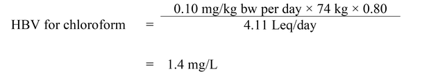
Figure 3 - Text description
The health-based value for chloroform is 1.4 mg/L. This is calculated by multiplying the tolerable daily intake of 0.10 mg/kg bw per day by the average adult body weight of 74 kg and by the allocation factor of 0.80. The product is then divided by 4.11 Leq/day which is the total exposure contribution from drinking water.
- 0.10 mg/kg bw per day is the TDI derived above
- 74 kg is the average adult body weight (Health Canada, 2021b)
- 0.80 is the allocation factor considering that drinking water is the main source for exposure to chloroform (Krishnan and Carrier, 2013)
- 4.11 Leq/day is the total exposure contribution from drinking water (see section 1.3.2, Multiroute exposure through drinking water)
Given that chloroform is a threshold carcinogen, exposures to chloroform levels below the HBV are considered to be protective of both non-cancer and cancer endpoints.
3.2 BDCM
The BMDL01 of 16.3 mg/kg bw per day, based on tumours in the large intestine (colon) of male rats (NTP, 1987; NTP, 2006), was selected as the point of departure. Using allometric scaling in order to represent human exposures, an HED was derived as follows:
Figure 4.
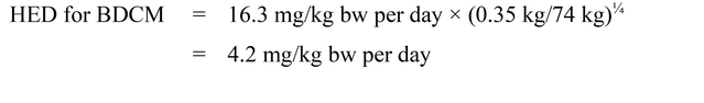
Figure 4 - Text description
The human equivalent dose for BDCM is 4.2 mg/kg bw per day. This is calculated by multiplying the BMDL01 of 16.3 mg/kg bw per day by the allometric scaling factor of (0.35 kg/74 kg)¼.
- 16.3 mg/kg bw per day is the BMDL01 identified for tumours in the large intestine of male rats (NTP, 1987; NTP, 2006)
- 0.35 kg is the average body weight of a rat (Health Canada, 1994)
- 74 kg is the average body weight of an adult human (Health Canada, 2021b)
- (0.35 kg/74 kg)¼ is the allometric scaling factor to account for interspecies differences in susceptibility to BDCM (U.S. EPA, 2011)
The HED was used to derive the cancer slope factor (CSF):
Figure 5.

Figure 5 - Text description
The cancer slope factor for BDCM is 0.002 (mg/kg bw per day) −1. This is calculated by dividing the 1% benchmark response by the human equivalent dose of 4.2 mg/kg bw per day.
- 0.01 is the 1% benchmark response
- 4.2 mg/kg bw per day is the HED calculated above
The dose associated with each lifetime risk is calculated by dividing the lifetime risk by the CSF of 0.002 (mg/kg bw per day)−1 (see Table 17). The estimated concentrations in drinking water corresponding to lifetime cancer risks are calculated using the following equation:
Figure 6.

Figure 6 - Text description
The health-based value for BDCM is calculated by multiplying the dose corresponding to the specific risk level by the average adult body weight of 74 kg. The product is divided by 3.55 Leq/day which is the total exposure contribution from drinking water.
- X is the dose corresponding to the risk level (see Table 17 below)
- 74 kg is the average body weight of an adult human (Health Canada, 2021b)
- 3.55 Leq/day is the total exposure contribution from drinking water (see section 1.3.2, Multi-route exposure through drinking water)
| Lifetime risk | Dose (mg/kg bw per day) | Estimated concentrations in drinking water (mg/L) |
|---|---|---|
| 10−4 | 10-4/0.002 (mg/kg bw per day)−1 = 0.05 | (0.05 mg/kg bw per day × 74 kg )/3.55 Leq/day = 1.04 |
| 10−5 | 10-5/0.002 (mg/kg bw per day)−1 = 0.005 | (0.005 mg/kg bw per day × 74 kg )/3.55 Leq/day = 0.104 |
| 10−6 | 10-6/0.002 (mg/kg bw per day)−1 = 0.0005 | (0.0005 mg/kg bw per day × 74 kg )/3.55 Leq/day = 0.0104 |
Since drinking water is the main source for BDCM, an excess lifetime cancer risk of 10−5 was used to derive an HBV of 0.100 mg/L or 100 µg/L (rounded) (Health Canada, 2021c).
As there is evidence of non-cancer effects following BDCM exposure, a non-cancer risk assessment was conducted for comparison. Using a BMDL10 of 0.777 mg/kg bw per day derived from liver effect data (fatty degeneration) in male rats from the Aida et al. (1992b) chronic study, a TDI of 0.008 mg/kg bw per day and an HBV of 0.133 mg/L were calculated. As the cancer risk assessment resulted in a more conservative value for BDCM in drinking water compared with that generated by the non-cancer approach, the cancer risk assessment was determined to be the most appropriate driver of the MAC in drinking water.
3.3 DBCM and bromoform
As indicated in section 2.5.3, Selected key studies for DBCM and bromoform, no key studies were selected for DBCM and bromoform and consequently no HBVs were calculated for these substances.
3.4 I-THMs
The limited toxicity data available for I-THMs preclude the derivation of an HBV for these substances.
3.5 Mixture assessment
A "[combined] exposure to multiple substances (mixture) Risk Assessment (CRA)" (adapted from WHO [2017a] and EFSA [2019]) was conducted to determine if the 4 THMs should be considered individually or together for risk assessment and management. The CRA also helps prioritize substances for further testing (by highlighting areas of uncertainty and identifying critical data needs). The I-THMs were not included in the mixture risk assessment since there are few to no data on their concentrations, toxicokinetics, hazard or mode of action. This type of information is required to determine if substances can be grouped together. In terms of the 4 THMs, based on the problem formulation (Appendix C), there is credible evidence of combined exposure to some or all of the chemicals, there is evidence of potential for adverse effects in humans, and there is the potential to cause toxicity in a similar way or affect the same organ(s). However, the key study used to derive the HBV for chloroform is based on a non-carcinogenic endpoint, while that for BDCM is based on a carcinogenic endpoint. There is limited guidance on whether an additive approach should be applied for carcinogens, and further whether hazard indices for non-carcinogens and carcinogens (that is, different modes of action) should be added together despite having some affected organs in common. Consequently, the CRA was examined at the problem formulation stage and not pursued further.
4.0 Analytical and treatment considerations
4.1 Analytical methods
4.1.1 Standardized methods to detect trihalomethanes
Standardized methods available for the analysis of individual THMs in drinking water and their respective method detection limits (MDLs) are summarized in Table 18. MDLs are dependent on the sample matrix, instrumentation and selected operating conditions, and they will vary between individual laboratories. These methods are subject to a variety of interferences, which are outlined in the respective references. For method EPA 551.1 Rev. 1, it was noted that both MTBE and pentane may contain observable amounts of chlorinated solvent (for example, chloroform, trichloroethylene and carbon tetrachloride) (U.S. EPA, 1995a).
Accredited laboratories in Canada were contacted to determine MDLs and method reporting limits (MRLs) for THM analysis. The MDLs were in the same order of magnitude as the range of those reported in Table 18. The MRLs ranged from 0.5 to 1.0 µg/L for chloroform, from 0.4 to 1.0 µg/L for BDCM, from 0.4 to 1.0 µg/L for DBCM, and from 0.2 to 2.0 µg/L for bromoform (AGAT Laboratories, 2020; City of Winnipeg, 2020; Metro Vancouver Laboratory, 2020; MOE, 2020; RPC, 2020; SRC Environmental Analytical Laboratories, 2020). The DLs from the PT data are in the ranges of 0.1 to 9.0 μg/L for chloroform, 0.07 to 2.0 µg/L for BDCM, 0.02 to 1.3 µg/L for DBCM, 0.08 to 2.0 µg/L for bromoform, and 0.3 to 30 µg/L for total THMs (see Table 2).
Drinking water utilities should discuss sampling requirements with the accredited laboratory conducting the analysis to ensure that quality control procedures are met. MRLs need to be low enough to ensure accurate monitoring at concentrations below the MAC.
| Method (Reference) | Methodology | MDL (µg/L) |
|---|---|---|
| EPA 502.2 Rev. 2.1 (U.S. EPA, 1995b) |
Purge-and-trap capillary column gas chromatography with photoionization and electric conductivity detectors in series (GC/PID/ELCD) |
|
| EPA 524.2 Rev. 4.1 (U.S. EPA, 1995c) |
Capillary column gas chromatography/mass spectrometry (GC/MS) |
|
| EPA 524.3 Rev. 1 (U.S. EPA, 2009) |
GC/MS |
|
| EPA 524.4 (U.S. EPA, 2013) |
GC/MS using nitrogen purge gas |
|
| EPA 551.1 Rev. 1 (U.S. EPA, 1995a) |
Liquid-liquid extraction and gas chromatography with electron-capture detection (LLE/GC/ECD) using
|
MTBE
|
Pentane
|
||
| SM 6040 B (APHA et al., 2018) |
Closed-loop stripping, gas chromatography/mass spectrometry (CLSA-GC/MS) |
|
| SM 6200B (APHA et al., 2018) |
Purge-and-trap capillary-column GC/MS |
|
| SM 6200C (APHA et al., 2018) |
Purge-and-trap capillary-column – GC method |
|
| SM 6232B (APHA et al., 2018) |
Liquid-liquid extraction – GC (LLE/GC) method | MDL depends on the characteristics of the gas chromatographic system. Method measures THM concentrations in the range OF 0.1 to 200 µg/L |
|
BDCM = bromodichloromethane, DBCM = dibromochloromethane, GC/MS = gas chromatography/mass spectrometry, MDL = method detection limit, MTBE = methyl tert-butyl ether, NA = not available |
||
4.1.2 Sample preservation and preparation
The analytical methods in Table 18 measure the concentration of individual THM compounds in the sample. The total THM concentration is calculated by summing the 4 individual THM concentrations and comparing them with the MAC.
Sample processing considerations for analysis of THMs in drinking water (that is, sample preservation, storage) using U.S. EPA methods can be found in the references listed in Table 18. In addition, SM 6010 B provides guidance on sample collection and preservation for the methods listed under American Public Health Association (APHA) Standard Methods(APHA et al., 2018). Appropriate sample handling procedures are essential to obtain accurate, precise and reliable data on THM occurrence and formation.
Once a sample is taken, it is critical to quickly stop further reaction with organic and inorganic precursors, which can continue to form more THMs. This is generally achieved by adding reducing (quenching) agents in excess to the water samples. THMs were not found to be susceptible to chemical degradation by reducing agents (Kristiana et al., 2014).
4.1.3 Online and portable meters
Commercial online and portable analyzers are available for quantifying individual THM compounds as well as total THMs (in 30 to 120 minutes depending on the analyzer). Analysis is generally based on purge-and-trap gas chromatographic technology although some devices use headspace or capillary extraction before gas chromatography. These analyzers can be used to obtain a rapid or near-continuous indication of THM concentrations. They can also be used to determine the potential of treated waters to form THMs in the distribution system. Real-time monitoring of THMs at various locations in the distribution system will allow for
- Optimization of treatment processes at the drinking water plant
- More targeted and efficient drinking water plant operations
- Identification of problematic areas (for example, inorganic/organic pipe deposits that cause increased levels of THM formation)
- Determination of flushing location and time in distribution system
- Water age evaluation in key locations in the distribution system
In general, these analyzers can measure individual THM compounds in the range of 2 to 80 µg/L or total THMs between 1 and 1,000 µg/L.
To ensure accurate measurements using these units, water utilities should develop a quality assurance and quality control program. This program should include periodic verification of results using an accredited laboratory. The devices should be calibrated according to manufacturer's instructions. Water utilities should check with the responsible drinking water authority to determine whether results from these units can be used for compliance reporting.
A colorimetric method is also available. It can be used for day-to-day operations and estimates THMs, based on chloroform content, using reagents and a spectrophotometer. This method has been demonstrated to have good correlation with standardized methods and has been used in small-scale systems (Ali et al., 2019). A few studies have used this method in assessing THM concentrations (Ahmed et al., 2019; Ali et al., 2019).
4.1.4 THM formation potential tests
Water utilities need to understand the source-specific reactivity of natural organic matter (NOM) when selecting a disinfectant to mitigate the formation of THMs (Hua and Reckhow, 2007a). Source-specific treatability studies, including THM formation potential (THMFP) methods, should be conducted when evaluating different mitigation measures and/or alternative treatment options. Formation potential methods are intended to evaluate water sources, water treatment processes and seasonal changes or to predict THM concentrations in the distribution system. All methods require a control of the parameters to obtain reproducible and meaningful results. These parameters include water temperature, pH, reaction time, and free chlorine doses and residuals (or monochloramine for a simulated distribution system [SDS] test) (Symons et al., 1981; Koch et al., 1991; Sketchell et al., 1995; Summers et al., 1996, APHA et al., 2018). These methods do not directly evaluate the impact of the drinking water system, pipe wall reactions, tank operations and other water quality factors.
Different methods to evaluate THMFP along with test conditions and various considerations are presented in Table 19. Formation potential test methods that use very high chlorine doses may not correctly determine differences in THM yield when bromide is present. This is because chlorine can out-compete bromine when in excess (Bond et al., 2014). Under typical operating conditions, bromine is much more effective at forming THMs than chlorine (Bond et al., 2014). The uniform formation conditions test (UFC) uses a typical chlorine dose and does not distort THM species formed. Therefore, the UFC test enables the direct comparison of results to assess the effectiveness of various treatment options (Summers et al., 1996; Reckhow and Singer, 2011).
| Methods | Test conditions | Comments | |
|---|---|---|---|
| Chlorine residual at the end of test | pH/ T0C/ Reaction time | ||
| SM 5710 B THMFP (APHA et al., 2018) |
3 to 5 mg/L | Standard reaction conditions: 7.0 ±0.2/ 25°C/ 7 days |
|
| SM 5710 C SDS-THM (APHA et al., 2018) |
Sample is disinfected to produce a residual level comparable to that of the finished drinking water | Test conditions (for example, temperature, pH, incubation time, bromide concentration, disinfectant dose and residual concentration) mimic local distribution system conditions |
|
| UFC test (Summers et al., 1996) |
1.0 ± 0.4 mg/L | 8.0 ±0.2/ 20°C/ 1 day |
|
| Hold Study (Alexander et al., 2019) |
Evaluated as part of test | DWDS pH/DWDS temperature/ 0.6, 12, 24, 48 and 96 hours |
|
| Br-THMs = brominated THMs, DWDS = drinking water distribution system, SDS-THM = Simulated distribution system Trihalomethanes, THMFP = Trihalomethane formation potential, UFC = uniform formation conditions | |||
4.2 Operational indicators of THM formation
Various operational parameters can be used as indicators of THM formation. These are not to be used to assess compliance with the MAC but provide alternative parameters that, depending on the indicator, may be measured more frequently. They may provide operators with additional information to assist in the management of THMs.
4.2.1 Specific ultraviolet absorbance
Specific ultraviolet absorbance (SUVA) has been used as an operational indicator of NOM character and effectiveness for NOM removal (AWWA, 2011; Health Canada, 2020a). SUVA is defined as ultraviolet (UV) absorbance at 254 nm (m-1) divided by the dissolved organic carbon (DOC) concentration (mg/L) (AWWA, 2011; Hua et al., 2015). Research has been conducted to determine how SUVA relates to NOM composition, to DOC and as a THM formation predictor (see Table 20). The effectiveness of SUVA as a THM predictor is water specific. As a bulk parameter, SUVA may not capture the heterogeneous nature of NOM (Ates et al., 2007; Hua et al., 2015; Marais et al., 2019).
| SUVA (L/mg·m) | NOM Composition | Typical components | Potential as THM precursor | SUVA to DOC | SUVA as THM formation predictor |
|---|---|---|---|---|---|
| < 2 | Mostly non-humic, hydrophilicTable 20 footnote a and low MW compounds | AOMTable 20 footnote b | Can be significant during presence of algal blooms | Weak correlation for MW < 1 kDa (SUVA may not effectively characterize NOM with lower MW) |
Weak correlation Non-humic and low SUVA NOM may contribute substantially to THM formation |
| Carbohydrates and sugars | Poor | ||||
| 2 to 4 | Mixture of humic and non-humic matter, mixture of hydrophobic and hydrophilic, with low to high MW | Fulvic acid | Significant | Strong correlation for MW > 1 kDa and greater correlation as MW increased | Strong correlation generally reported in the literature |
| > 4 | Mostly aquatic humics; hydrophobic and high MW compounds | Humic acid | Primary | Strong correlation for MW > 1 kDa and greater correlation as MW increased | Strong correlation generally reported in the literature |
|
AOM = algal organic matter, DOC = dissolved organic carbon, MW = molecular weight, NOM = natural organic matter, SUVA = specific ultraviolet absorbance Sources: Plummer and Edzwald, 2001; Kitis et al., 2001, 2002, 2004; Liang and Singer, 2003; Rodriguez et al., 2004; Ates et al., 2007; AWWA, 2011; Edzwald and Tobiason, 2011; Chowdhury, 2013c; Hua et al., 2015; Pivokonsky et al., 2016; Ding et al., 2019; Marais et al., 2019 |
|||||
4.2.2 Differential UV absorbance
Differential UV absorbance (DUVA)-DBP relationships have the potential to provide a relatively simple method to estimate DBP concentration and better inform operational decisions. DUVA evaluates the difference in UV absorbance at specific wavelengths (typically 272 nm) before and after the chlorination of a sample and correlates it to DBP occurrence (Korshin et al., 2002; Roccaro et al., 2009; Özdemir et al., 2013; Beauchamp et al., 2018, 2019; Guilherme and Dorea, 2020).
Several bench-scale studies determined relationships between DUVA (272 nm wavelength) and various DBPs (for example, THMs and HAAs), before and after chlorination, with good correlation (R2 > 0.65 for THMs) (Korshin et al., 2002; Roccaro et al., 2009; Özdemir et al., 2013; Beauchamp et al., 2018; Guilherme and Dorea, 2020). These studies found that the relationship was site specific and varied seasonally. However, it was not determined if these same relationships would hold from year to year (Beauchamp et al., 2018). The DUVA-DBP relationship determined at full-scale differed from those seen at lab-scale. A study found multiple regression parameters (DUVA measured at various wavelengths, and UV absorption) resulted in a more widely applicable relationship between DBP concentration and DUVA (Beauchamp et al., 2019). A bench-scale study by Guilherme and Dorea (2020) indicated the importance of developing this relationship at a range of DBP concentrations that would be expected to occur.
4.2.3 Fluorescence
Fluorescence is a rapid NOM classification method that shows promise. However, research is still ongoing to determine how the method can be integrated as a routine monitoring tool (McKnight et al., 2001; Fellman et al., 2010; Bridgeman et al., 2011; Markechová et al., 2013; Murphy et al., 2013; Sanchez et al., 2013; Wright et al., 2016; Peleato et al., 2017; Frank et al., 2018; Li et al., 2020a).
4.2.4 Total organic halogen and unknown total organic halogen
Total organic halogen (TOX) is used to characterize the incorporation of a halogen into organic molecules (Kristiana et al., 2009). TOX includes THMs, HAAs, haloacetonitriles and any other known or unknown halogenated DBP. TOX is a parameter used in some studies to assess the overall impact of a treatment or operational change on all halogenated DBPs. Unknown total organic halogen (UTOX) represents the unknown halogenated DBPs in the water.
4.3 Source water considerations
Seasonal variations and climate change can impact source water quality, both in terms of NOM and inorganic precursors. Changes in source water quality can subsequently influence the amount and reactivity of NOM, and impact treatment effectiveness and the potential for THM formation.
4.3.1 Seasonal changes
Waters have different sources of NOM and precursors that change seasonally, affecting THM formation (Li and Mitch, 2018). There are variations in temperature, NOM structure and concentration, inorganics concentrations and pH (Reckhow and Singer, 2011). Higher THM concentrations have generally been found to occur during summer and fall months (see Table 21).
NOM changes seasonally due to a variety of factors that include snowmelt, leaf-off, temperature changes and temperature-driven microbial metabolism (Zhao et al., 2018). In spring, there may be heavy rainfall events that lead to a rise in allochthonous, hydrophobic NOM. In summer, algal blooms can increase autochthonous, hydrophilic NOM. In fall, leaf litter waste adds terrestrial NOM to waterways (Reckhow and Singer, 2011). Temperature changes impact chlorine decay, the THM formation rate and seasonal changes in NOM and inorganics all have an impact on THMs formed.
Awad et al. (2017) examined seasonal changes between river and reservoir water. It was observed that changes in average DOC, %DOC removed by alum coagulation and THMFP was higher for river water than for reservoir water. Storage of large volumes of water in a reservoir enables mixing of influent water and stabilization of water quality.
Westerhoff et al. (2022) reported that seasonal changes in bromide are related to streamflow. Higher bromide levels were reported for lower streamflow.
Rainfall events can result in overland flow of contaminants to surface water. This is offset by increased flowrate, resulting in dilution (Clark et al., 2007). Changes in NOM quality and quantity during and after rainfall events can lead to THM variations in the distribution system (Delpla and Rodriguez, 2016). Generally, higher total organic carbon (TOC) was found in filtered water during and after rainfall events. This resulted in increased chlorine and alum doses to compensate for these changes. Studies evaluating impacts of rainfall events are presented in Table 21.
| Location | Systems | Parameter | Comments | Reference |
|---|---|---|---|---|
| Seasonal effects | ||||
| QC and NL Sep 2010 to Oct 2011 |
25 small systems | THM | Highest in summer and fall. | Scheili et al. (2015) |
| ON | 3 systems | THM | Higher between June and November and lower between December and April. | Chowdhury (2013c) |
| QC Apr to Nov 1998 |
4 mid-size systems | THM |
|
Rodriguez and Sérodes (2001) |
| QC 14-month period |
1 system | TOC |
|
Rodriguez et al. (2004) |
| THM | Fall level 5 times higher than winter. | |||
| Scotland 1-year period |
5 systems | THM | Peak in September (more than double that in March). | Valdivia-Garcia et al. (2019) |
| 6 European countries | 13 systems | THM |
|
Krasner et al. (2016b) |
| Rainfall events | ||||
| QC 22 rainfall events (Apr to Oct 2017) |
1 system (11d dry period – 5d wet period – 19d dry period) |
UV254 absorbance |
|
Delpla et al. (2023) |
| Turbidity |
|
|||
| 1 system (Heavy precipitation sequence of 33 days) |
UV254 absorbance |
|
||
| QC 4 rainfall events |
2 systems | THM |
|
Delpla and Rodriguez (2016) |
| QC 4 rainfall events |
1 system | Cl- and Br- |
|
Delpla and Rodriguez (2017) |
| TOC | Somewhat higher during and post-rainfall, causing increased chlorine demand and alum dose. | |||
| THM | Increased during and post-rainfall event. | |||
| Br-THMs = brominated THMs, NL = Newfoundland and Labrador, QC = Quebec, TOC = total organic carbon, UV254 = UV absorbance at 254 nm wavelength | ||||
4.3.2 Climate change impacts
Climate change is expected to continue to raise water temperatures and cause frequent, longer-lasting and more intense extreme weather events and associated natural disasters. These events will result in heavy precipitation, floods, heatwaves, droughts and wildfires (Takaro et al., 2022; Government of Canada, 2023). Additionally, atmospheric acid deposition has been reduced over the last number of decades. This has resulted in the recovery from acidification by increasing pH and acid neutralization capacity (or alkalinity) of surface waters (Anderson et al., 2023). Increased NOM concentrations with more hydrophobic character have been associated with this recovery in water quality.
Climate change impacts are expected to change the nature and quantity of NOM in source waters (see Table 22) (Anderson et al., 2023). These changes in source water quality will have potential treatment implications. NOM may not be adequately removed under current treatment conditions, which dictates the need for water systems to adjust their treatment strategy when changes in DBP precursors are noted. A review of impacts on various treatment processes is presented in Anderson et al. (2023).
A good resource for climate change discussion in relation to water treatment and the importance of creating and maintaining a climate action plan is presented in the American Water Works Association's (AWWA) Climate Action Plans – Adaptive Management Strategies for Utilities (AWWA, 2021).
| Event | Considerations |
|---|---|
| Temperature change |
|
| Flooding | Increases sediment and contaminant loading to rivers and lakes. |
| Extended growing seasons | Alter catchment soil and vegetation, which impacts storage and leaching of dissolved organic matter and sulphate in watersheds. |
| Drought periods |
|
| Sea level rising | Seawater intrusion into wells with elevated concentrations of bromide. |
| High frequency rainfall events |
|
| Wildfires |
Frequency is on the rise and has potential to impact source water quality. Catchment hydrology may be impacted through altering:
|
|
|
|
|
|
AOM = algal organic matter, DBP = disinfection by-products, DOC = dissolved organic carbon, NOM = natural organic matter, THMs = trihalomethanes Sources: Whitehead et al., 2009; Liao et al., 2015; Wang et al., 2015a, b; Kolb et al., 2017; Ruecker et al., 2017; Seidel et al., 2017; Poon and Kinoshita, 2018; Chow et al., 2019; Hohner et al., 2019; Chen et al., 2020; Majidzadeh et al., 2020; Skwaruk et al., 2020; Uzun et al., 2020; Anderson et al., 2023 |
|
Studies showing the impacts of extreme events on THM formation are presented in Table 23. More detailed discussion of potential impacts to NOM from climate change can be found elsewhere (Ritson et al., 2014; Anderson et al., 2023). Treatment facilities may benefit from early warning systems that alert operators to source water changes linked to extreme weather events, allowing for treatment to be adjusted accordingly (Barry et al., 2016).
| Event | Systems | Parameter | Comments | Reference |
|---|---|---|---|---|
| North Carolina and South Carolina flooding (2016) | 18 sub-watersheds | THMFP |
|
Majidzadeh et al. (2020) |
| Hurricane Matthew (2016) |
2 sites | THMFP |
|
|
| Hurricane Joaquin (2015) |
Water collected from river | THMFP |
|
Ruecker et al. (2017) |
| Post-wildfires | 23 catchments | # of violations of THM > 80 μg/LTable 23 footnote a (2-year window) |
|
Pennino et al. (2022) |
| THM | Maximum post-fire was 0.21 mg/L. | |||
| 127 catchments | THM (1-year period) |
|
||
|
Hayman Fire in Colorado (2002) Samples: October 2014 to September 2016 |
13 catchments
Moderately burned ≡ < 50% area Extensively burned ≡ > 74% area |
General | Impacts persisted over 14 years. | Chow et al. (2019) |
| DOC |
|
|||
| THM |
|
|||
| Nitrogen | Extensively burned catchments – lower DOC/N. | |||
| Bromide | Moderately burned catchments – lowest incorporation of bromide into THMs. | |||
| Northern California 2 fires (2015) |
3 watersheds (burn areas: 0%, 20% and >90%) | THM |
|
Uzun et al. (2020) |
|
Br-THM = brominated trihalomethanes, DOC = dissolved organic carbon, N = nitrogen, SUVA = specific ultraviolet absorption, THMFP = Trihalomethane formation potential |
||||
4.4 THM formation
Chlorinated DBPs like THMs and HAAs are formed when chlorine reacts with organic and inorganic precursors. The type and amount of THMs that form depend on numerous factors such as:
- Organic precursors (for example, NOM)
- Inorganic precursors (for example, bromide and iodide)
- The oxidation and disinfection strategy
- pH
- Water temperature
- Reaction time
(Liang and Singer, 2003; Baribeau et al., 2006; Srivastav et al., 2020)
There are 2 natural sources of NOM: allochthonous and autochthonous (Reckhow and Singer, 2011). Allochthonous NOM is generally derived from terrestrial plants and can consist of humic and fulvic acids (generally hydrophobic compounds). This type of NOM is transported to surface water through runoff events. Autochthonous NOM includes algal biomass and algal organic matter (AOM) (generally hydrophilic compounds) (Zhao et al., 2018). Anthropogenic (human) activities can also contribute to NOM. The amount and species of THMs formed are a function of water quality parameters (for example, type and amount of NOM, inorganic precursors, pH, temperature), usage of oxidants and disinfectants, and contact time (water age). THMs continue to form over time with reaction between precursors and disinfectants (Becker et al., 2013; Liu et al., 2013).
4.4.1 Organic precursors
NOM is an extremely complex mixture of organic compounds and is found in all groundwater and surface waters. NOM can impact processes designed to remove or inactivate pathogens, contribute to the formation of DBPs and favour the development of biofilms in the distribution system. The treatability and reactivity of NOM vary significantly in Canada, as each water source has unique features.
Halogenated DBP formation, like THMs, is generally known to increase with the "activated" (defined as electron-rich) aromatic content of NOM (Liang and Singer, 2003). There may be a strong relationship between DOC and THM formation. However, this relationship becomes weaker when comparing different source waters. NOM character will change based on ecoregion, lake recovery from acid rain, climate change and seasonal variations (Reckhow and Singer, 2011; Anderson et al., 2023).
High SUVA, hydrophobic NOM (for example, humic acids and fulvic acids) are known THM precursors. However, lower SUVA, hydrophilic NOM may also contribute substantially to THM formation (see Table 20). When chloramination was used, there was a lower correlation between SUVA and THMs formed. This result indicated that chloramines react with a wider range of precursors than chlorine (Hua et al., 2015).
NOM consists of numerous organic compounds that can be measured directly, using methods that are generally complex. However, there are several other parameters that can be used to provide an indication of the concentration and character (that is, chemical, physical and biodegradability properties) of NOM (see Appendix D). These parameters include TOC, DOC, UV absorption and chemical oxygen demand (COD) (Health Canada, 2020a). TOC and DOC are related to the quantity of organic carbon. In freshwater systems, UV absorption can be used to characterize the quality and quantity of NOM (Delpla et al., 2023). SUVA can be used to characterize the type of NOM present (see Table 20). Chemical oxygen demand serves to give some indication of the concentration of oxidizable organic matter in a water sample (Frisch and Kunin, 1960; Stoddart and Gagnon, 2014). It is important to understand variations in NOM concentrations and character to select, design and operate appropriate water treatment processes and disinfection.
Several studies have shown that lower THM levels are formed with chloramine than chlorine (Hua and Reckhow, 2008; Bougeard et al., 2010; AWWA, 2017; Mayer and Ryan, 2019; Mazhar et al., 2020). THM formation with chloramines generally remains stable with contact time, pH and temperature and increases with dose (Hong et al., 2013).
When algal blooms are present, there is an increase in algae cells and AOM. AOM can release extracellular organic matter (EOM) and, through cell lysis, intracellular organic matter (IOM) (taste and odour compounds and cyanotoxins). Some studies report that terrestrial NOM produces more THMs than those from AOM due to AOMs' lower aromaticity during chlorination or chloramination (Plummer and Edzwald, 2001; Fang et al., 2010a, b; Li and Mitch, 2018; Zhao et al., 2018; Liu et al., 2020a). However, one study stated that certain algal populations result in higher THM formation (Seidel et al., 2017). Higher nitrogen in AOM could promote nitrogeneous DBPs (Li and Mitch, 2018).
THM formation during chlorination of water with AOM depends on algae type and growth phase (Plummer and Edzwald, 2001). There is poor removal of algal cells and AOM through conventional water treatment processes (Huang et al., 2009; Pivokonsky et al., 2012, 2016; Dong et al., 2021). When determining the oxidation or disinfection strategy for water with AOM, it is important to understand the individual contributions of EOM and IOM from the different algae species (Liao et al., 2015).
Pre-chlorination will inactivate algae cells and lyse them, which releases IOM, and high molecular weight (MW) organics will be degraded to low MW organics (Chen et al., 2009; Ma et al., 2012, 2019). This release of THM precursors impacts treatment. Bench-scale studies evaluated pre-chlorination of water with various algae species followed by conventional treatment and post-chlorination. These studies generally showed that at lower chlorine doses (0.5 mg/L), THM formation declined compared to that without pre-chlorination. As the chlorine dose increased (2 mg/L and 4 mg/L), THM formation increased beyond that of treatment without pre-chlorination. The higher pre-chlorination dose can cause a larger IOM release, having a negative impact on the effectiveness of coagulation and sedimentation (Ma et al., 2012; Qi et al., 2016).
Biofilms can develop within the distribution system and provide a reservoir of DBP precursor material that is distinctive (Abokifa et al., 2016; Xu et al., 2018; Li et al., 2020c). NOM in the distribution system water can transfer to the biofilm, followed by biotransformation and possible detachment (Wang et al., 2012; Abokifa et al., 2016). Positive correlation of microbial inactivation and THM formation indicates that bacterial cell breakdown is another precursor (Wang et al., 2013, 2021). The quantity, physical structure and chemical composition of the biofilm can affect the transport and penetration of disinfectant. This biofilm can survive and have viable cells remain under constant disinfectant exposure (Xue et al., 2014; Liu et al., 2016; Wang et al., 2021). Biofilm development and biological growth may result in biological instability in the distribution system. These systems are more likely to have unstable disinfectant residual, possibly resulting in chlorine addition and therefore increased THM formation.
Further information on NOM is available in Health Canada's Guidance on Natural Organic Matter in Drinking Water (referred to herein as NOM guidance document) (Health Canada, 2020a).
4.4.2 Inorganic precursors
The presence of inorganic precursors, such as bromide and iodide, impacts the type of THMs that are formed. The presence of bromide may result in the formation of Br-THMs, while the presence of iodide in water may result in the formation of I-THMs. (Tugulea et al., 2018). The presence of ammonia will also have an impact as it will react with chlorine to form monochloramine. The change of disinfectant will alter the amount and type of THMs formed.
Other water constituents, such as salts and hardness, may have an impact on THM formation. Generally, the impacts of these constituents were lower when tested in a surface water than distilled water (see Appendix E).
4.4.2.1 Bromide
When bromide is present, there is a shift to the formation of Br-THMs (bromoform, DBCM, BDCM) (Summers et al., 1993; Symons et al., 1993; Chowdhury et al., 2010; Hu et al., 2010; Liu et al., 2013; Roccaro et al., 2014; Krasner et al., 2016a; Neil et al., 2019). When oxidized with chlorine, bromide forms hypobromous acid (HOBr) and hypobromite ion (OBr-). HOBr has more powerful halogenating activity, reacts faster and attacks more sites in the organic precursor than hypochlorous acid (HOCl). The remaining HOCl continues to react with any residual Br- to form more HOBr (Symons et al., 1993; Hua and Reckhow, 2013; Tian et al., 2013; Neil et al., 2019). HOBr reacts with NOM to form Br-THMs as well as other brominated DBPs (Hua and Reckhow, 2013). The lowest HOBr formation is related to the lowest bromide concentration (Westerhoff et al., 2022). An increase in bromide concentration may result in an increase in total molar concentration of THMs (sum of chloroform and Br-THMs) (Chowdhury, 2013c).
The bromine incorporation factor (BIF) is used to determine the amount and type of Br-THMs that are formed. The BIF is defined as the molar ratio of Br-THMs to total THMs. The ratio ranges from 0 (all chloroform) to 3 (all bromoform) (Krasner et al., 2006; Hong et al, 2013). The BIF can be used to assess any changes in source water, treatment and/or distribution system conditions. Treatment can remove hydrophobic NOM. However, bromide is not easily removed, resulting in increases in Br-/DOC and Br-/free available chlorine. Increases in these ratios cause a rise in BIF, indicating more Br-THMs formed (Summer et al., 1993; Symons et al., 1993; Chiu et al., 2012; Liu et al., 2013; Krasner et al., 2016a; Zhang et al., 2017; Neil et al., 2019; Health Canada, 2020a). With chloramines, BIF also increases, but to a lower extent (Hong et al., 2013). The lower MW, hydrophilic NOM that is not well removed through treatment is more reactive with bromide, also leading to more Br-THM species (Kitis et al., 2002; Liang and Singer, 2003; Chowdhury, 2013c).
In the presence of bromide, chloramines can form bromamine, which leads to poor disinfection capabilities and chloramine instability (AWWA, 2017). Bromide reacts with chloramines to form HOBr, which can lead to Br-THM formation. Chloramines are unstable at near neutral pH values due to autodecomposition reactions. These reactions can be catalytically increased by bromide (AWWA, 2017).
4.4.2.2 Iodide
Currently, there are a lot more studies on chloroform and Br-THMs than on I-THMs. The understanding of the impact of iodide on the formation of THMs will improve as research continues. To date, no meaningful correlation has been found between bromide and iodide concentrations in source waters (Tugulea et al., 2018; Westerhoff et al., 2022). Br-/I- mass ratios from source waters in the U.S. and Canada ranged between 2.9 and 238 (Richardson et al., 2008; Weinberg et al., 2011). Iodide concentration in source waters may have a high seasonal variability. An iodide/total iodine ratio of 34.4% was observed in the winter and 86.6% in the summer (Tugulea et al., 2018).
The reaction rate constants for the oxidation of iodide and hypoiodous acid (HOI) by different oxidants are highly variable. It is predicted that the "probability" of I-THM formation increases in the order ozonation < chlorination < chloramination (Kumar et al., 1986; Fábián and Gordon, 1997; Bichsel and Von Gunten, 1999). Iodide can be oxidized to HOI acid and subsequently to iodate (IO3-), which is the desired sink as it will not react further to form I-THMs (Bichsel and Von Gunten, 2000).
HOCl/OCl- will rapidly oxidize iodide to HOI and subsequently to IO3- (Ullman et al., 1990; Bichsel and Von Gunten, 1999). The oxidation reaction rate of iodide to HOI is faster than that of HOI to IO3-. Subsequent reactions of HOI with NOM are responsible for the formation of I-THMs (Bichsel and Von Gunten, 1999, 2000; Richardson, 2003, 2008; Hua et al., 2006; Hua and Reckhow, 2007b, 2008; Gallard et al., 2009; Jones et al., 2012a, b; Ye et al., 2012; Allard et al., 2013; Zhang et al., 2015a, 2016, 2018b; Liu et al., 2017, 2018; Dong et al., 2019a). With a chlorine dose of 0.5 mg/L, all I-THMs increased and then declined as the chlorine dose increased to 5.0 mg/L (Hua et al., 2006). The authors stated that a possible strategy to control I-THMs is to increase the chlorine dose. However, adequate disinfection CTFootnote 1 may limit flexibility. Also, an increased chlorine dose can increase formation of chloroform and Br-THMs.
ClO2 rapidly oxidizes iodide to iodine (I2), leading to the formation of HOI, iodide and tri-iodide ion, and then I-THMs (Smith et al., 2010; Ye et al., 2013; Zhang et al., 2015a). When followed directly by chloramine, pre-oxidation with ClO2 reduced TIM and CDIM formation compared with chloramination alone (Jones et al., 2012b).
With chloramine, the oxidation of HOI to IO3- is a very slow process, extending the reaction time between HOI and NOM. The increased time leads to more I-THM formation, especially iodoform (Bichsel and Von Gunten, 2000; Hua and Reckhow, 2007b). The chloramination strategy (chlorine added before ammonia vs. preformed chloramine), and pre-chlorination strategy (chlorine dose and contact time) is an important factor (Bichsel and Von Gunten, 2000; Krasner et al., 2006; Hua et al., 2006; Hua and Reckhow, 2008; Richardson et al., 2008; Goslan et al., 2009; Jones et al., 2011, 2012a; Karanfil et al., 2011; Criquet et al., 2012; Allard et al., 2013; Liu et al., 2017).
Pre-oxidation with potassium permanganate, followed by chloramine, resulted in an increased amount of TIM and brominated I-THMs compared with chloramine alone (Jones et al., 2012b). The reduction product, manganese dioxide, may catalyze iodinated DBP formation in water with iodide for pH from 5.0 to 7.0 (Gallard et al., 2009). Ozone oxidation occurs very quickly to form IO3-, reducing I-THM formation (Bichsel and Von Gunten, 1999; Liu and Reckhow, 2001; Allard et al., 2013). UV has been shown to convert IO3- (stable form) into iodide (I-THM precursor) during post-chloramination (Liu et al., 2012a; Zhang et al., 2016, 2018b; Xia et al., 2018). UV application should be considered carefully for water containing IO3-.
In bromide-containing water, HOBr accelerates the oxidation process of HOI to IO3- in a bromide-catalyzed process. This more rapid reaction to IO3- results in reduced formation of I-THMs (Criquet et al., 2012; Liu et al., 2017). However, HOBr can lead to more brominated precursors that can react with HOI, possibly shifting to more brominated I-THM species (Westerhoff et al., 2004; Criquet et al., 2012).
4.4.3 Additional factors
Water quality parameters such as pH and temperature affect THM formation. It is important to understand the consequences of pH changes on the formation of all THM species and other DBPs (Chowdhury, 2013c). An increase in pH can increase chloroform formation (Reckhow et al., 1990; Liang and Singer, 2003; Li et al., 2007; Fu et al., 2009; Hu et al., 2010, 2019; Reckhow and Singer, 2011; Liu et al., 2011; Becker et al., 2013; Chowdhury, 2013c; Hong et al., 2013; Hua et al., 2015; Zhang et al., 2018c; Carra et al., 2020), yet can decrease Br-THM formation (Chowdhury, 2013c). If there is bromide in the water, reducing the pH to decrease chloroform formation will result in increased Br-THMs. This THM management strategy may also increase corrosivity of water, resulting in metal release (for example, lead, copper) or, in the presence of ammonia, result in the formation of dichloramine, which can cause taste and odour issues. Ideally, a management strategy will determine the pH that would minimize corrosion and other potential negative impacts as well as both the concentrations of THMs and the toxicity of the species formed.
At a higher water temperature, reaction rates are increased and decomposition of aromatic halogenated DBPs into THMs is enhanced (Reckhow and Singer, 2011; Becker et al., 2013; Hong et al., 2013; Hu et al., 2019; Valdivia-Garcia et al., 2019). The reaction is limited by higher chlorine decay with a warmer temperature. However, in practice, additional chlorine doses would be added to maintain residuals (Rodriguez and Sérodes, 2001; Reckhow and Singer, 2011). The impact of temperature on THM formation in the distribution system is not always direct. For instance, during summer when water temperatures are highest, water demand is generally also greater. This increased water demand results in lower water age and contact time in the distribution system (Becker et al., 2013). Disinfectant residual within the distribution system can also be impacted by temperature rises due to higher reaction rates, increased biological activity and variations in NOM (AWWA, 2017). Changes in water temperature should be considered together with other parameters that also vary seasonally, such as NOM quantity and composition.
THMs continue to form over time. Residence time is a function of water quantity and usage and can be subject to changes over time. These changes in residence time may coincide with water quality variations, which can compound the effect on THM formation. Overall, water quality and water quantity should both be examined to understand the potential impacts on THM concentrations.
4.5 Treatment considerations
Water utilities must balance effective disinfection against the creation of THMs because drinking water must, first and foremost, be microbiologically safe to prevent waterborne disease. For THM control, the preferred and most effective option is to reduce or limit its formation prior to and during distribution. At the water treatment plant, THMs are limited by removing NOM from water before chlorination, optimizing the disinfection process or changing the disinfection strategy. In situations where THMs have formed, there are options to remove them. This is generally not as effective as reducing their formation and should only be considered as an interim strategy while improved treatment is being evaluated.
4.5.1 Municipal-scale treatment
Strategies to reduce formation include precursor removal prior to disinfection, the use of alternative pre-oxidation or change in disinfection practices. Treatment may change seasonally or temporally to account for changes in factors that affect THM formation.
Technologies used to remove already formed THMs include aeration, granular activated carbon (GAC) or membrane filtration. Aeration can be conducted at booster/pump stations or in reservoirs. GAC or membrane filtration can be part of the treatment train within the treatment plant. Generally, chloroform is better removed through aeration and Br-THMs are better removed through GAC adsorption and reverse osmosis.
Any changes to control/minimize THMs needs to be evaluated using bench- and pilot-scale testing to ensure that treatment goals are met, effective disinfection is achieved and the change does not result in unintended consequences and challenges in complying with other regulatory requirements. These tests need to be repeated regularly to account for source water quality changes, seasonal variability and climate change.
4.5.1.1 Precursor control options
Organic precursor removal
Removal of organic precursors can minimize the formation of THMs. Coagulation followed by clarification or filtration is the most commonly used method, as it is effective in most applications. However, its applicability should be carefully analyzed on a source-specific basis because coagulation can only remove some NOM fractions; the remaining fractions may react with disinfectants such that other DBP drinking water guidelines are not achieved. In general, high SUVA (> 4 L/mg∙m) NOM tends to be hydrophobic in nature and is generally amenable to coagulation. Low SUVA sources tend to have NOM that is hydrophilic and not amenable to coagulation (Pernitsky, 2003). However, some hydrophilic neutral fractions can have a high SUVA, which can be misleading with respect to the potential for organic carbon removal using coagulation (Edzwald, 1993). If the post-coagulation DOC residual remains reactive, other technologies targeting the removal of specific NOM fractions may be necessary (Bond et al., 2011). As humic and fulvic acids are important DBP precursors, adequate colour removal may be necessary.
Enhanced coagulation has multiple objectives, including maximizing removal of particles and turbidity, as well as TOC and DBP precursors. Another objective is minimizing residual coagulant, sludge production and operating costs (White et al., 1997; Edzwald and Tobiason, 1999). Enhanced coagulation is generally carried out by depressing coagulation pH with higher coagulant doses (Gregory, 1998). A full-scale study evaluated enhanced coagulation to maximize organic precursor removal using UV254 monitoring to determine a dose adjustment strategy (Beauchamp et al., 2020). On a wider range of water, the results showed that an alum/UV254 stoichiometric dose of 180 ± 25 mg alum cm/L maximized the removal of DBP precursors. This relationship was found to hold in all seasons despite changes in water quality.
GAC can remove THM precursors and THMFP breakthrough generally parallels DOC breakthrough. Sometimes, the THMFP breakthrough lags that of DOC, making DOC a good surrogate parameter to monitor to determine when GAC needs to be regenerated (Reckhow and Singer, 2011). A few studies examined GAC with various disinfectants/oxidants and locations of implementation. One study showed that adding chlorine during GAC filtration extended the breakthrough time of the column over GAC with post-chlorination. With bromide, the results were improved; authors indicated that GAC better adsorbs the brominated DBPs over chlorinated DBPs (Jiang et al., 2017). A pilot-scale study evaluated 3 scenarios: GAC alone, pre-chlorination and pre-ozonation/GAC filtration. Each scenario reached breakthrough of THMs at similar bed volumes (BVs) (Verdugo et al., 2020). Following conventional treatment with GAC allowed for a lower chlorine dose for disinfection and better control of THMs and other DBPs during extreme rainfall events (Neil et al., 2019).
Ion exchange (IX) using a strong base anion exchange resin can potentially remove NOM (Reckhow and Singer, 2011; Health Canada, 2020a). However, frequent regenerations produce large volumes of high concentration brine, which creates disposal issues (Amini et al., 2018; Wright, 2022). Management/shipment of regenerant chemicals may also be an issue for small and/or remote drinking water treatment systems (Amini et al., 2018). Biological ion exchange (BIEX) is a promising technology. It uses naturally developing biofilm, formed by microbes in the raw water source, that consume the attached DOC (Zimmerman et al., 2021). This technology also uses a strong base anion exchange resin but has fewer regeneration cycles (months rather than days), thus resulting in less spent brine while reducing NOM. Several bench- and pilot-scale studies evaluated BIEX and the factors that affect performance; they showed successful removal of DOC and DBP precursors (Amini et al., 2018; Liu et al., 2020b, 2022; Edgar and Boyer, 2021; Zimmerman et al., 2021, 2023; Wright, 2022; Lee et al., 2023). A review of IX regenerant brine management issues and strategies are presented in Liu et al. (2021a).
IX may result in corrosion. Examples include galvanic corrosion driven by a chloride-to-sulphate mass ratio in the finished water (Edwards et al., 1999; Edwards and Dudi, 2004; Edwards and Triantafyllidou, 2007; Health Canada, 2022a); a reduction in pH from freshly regenerated ion exchange resin due to removal of bicarbonate ions during the initial BVs of a run (Clifford, 1999; Wang et al., 2010; Clifford et al., 2011); and a continual decease in pH due to frequent regeneration of an ion exchange resin. One study examined bicarbonate as an alternative to chloride for IX for reducing corrosion potential and it showed similar DBP precursor reduction (Fernandez et al., 2021). Mitigation strategies to address potential corrosion issues should be considered; information can be found elsewhere (Health Canada, 2022a).
Adsorption and IX processes are limited by media capacity and the effect of competing ions. Their performance will be affected by backwash frequency and media regeneration or replacement.
Health Canada's (2020a) NOM guidance document provides a more detailed discussion of the various treatment technologies (coagulation, reverse osmosis [RO], nanofiltration [NF], coagulation followed by microfiltration or ultrafiltration, IX, activated carbon or biological treatment) that can be used to remove NOM. Different treatment technologies exhibit different selectivity in precursor removal. The removal of NOM depends on the MW and the hydrophilic/hydrophobic properties (Zhang et al., 2017; Andersson et al., 2020). Hydrophobic NOM (high SUVA water) is typically more amenable to removal through treatment, whereas hydrophilic NOM is more difficult to treat (Chow et al., 2004, 2006). Treatment performance achieved using various treatment technologies can be found in Appendix F. Collectively, full-, pilot- and bench-scale results indicate that various treatments can be effective (Health Canada, 2020a). However, poor results can also be observed.
The choice of treatment and development of an effective NOM control strategy depends on many factors and needs a good understanding, including (Health Canada, 2020a):
- The type of NOM and variations in the concentration and character of NOM in the source water, including those due to seasonal changes, climate change, landscape changes or source water protection programs
- NOM's impact on water treatment processes and the impact of water treatment on NOM, for the full range of water quality conditions
- Interactions with other water constituents (for example, bromide and iodide)
- Interactions with treatment chemicals
- Interactions with processes (for example, fouling of membranes)
- Potential impacts on distribution system water quality, downstream water systems and users
Additional or alternative treatment options to enhanced coagulation for NOM removal include nanofiltration, coagulation/ultrafiltration, IX, GAC or powdered activated carbon (PAC), biological filtration and oxidation processes. These findings demonstrate the need to conduct proper testing to confirm sufficient NOM and DBP precursor removal and to optimize operational parameters. For coagulation, this includes jar testing. For other treatment technologies, this includes bench- and/or pilot-testing. Seasonal and temporal changes necessitate monitoring to ensure that the technology is optimized over a full range of water quality conditions.
The RO and NF process limitations may include membrane scaling and fouling as well as higher energy use and capital costs. Calcium, barium and silica can cause scaling and decrease membrane efficiency. Since RO completely removes alkalinity in water, it will continually lower treated water pH and increase its corrosivity. Therefore, the treated water pH must be adjusted and alkalinity will most likely need to be increased to avoid corrosion issues in the distribution system such as the leaching of lead and copper (Schock and Lytle, 2011; U.S. EPA, 2023).
Inorganic precursor removal
Removal of inorganic precursors like bromide and iodide can also be used to reduce formation of Br-THMs and I-THMs. Bromide is difficult to remove from water and although technically feasible, is unlikely to be a cost-effective option to reduce Br-THMs (Health Canada, 2018). An overview of bromide removal strategies, including bench- and pilot-scale studies, is presented in Westerhoff et al. (2022). The authors indicate the necessity for significant improvements in bromide removal capacities to have these and other technologies viable at full scale. Drinking water systems should have a good understanding of the sources and concentration of bromide in their source waters and seasonal variability.
The removal of iodide may be achieved by oxidation to IO3- (stable compound that does not form I-THMs). Pre-chlorination and pre-ozonation are 2 options that can oxidize I- to IO3- and avoid formation of I-DBPs (Allard et al., 2015; Kimura et al., 2017). However, pre-chlorination may form other DBPs. To provide effective oxidation of I- to IO3-, pre-chlorination contact time prior to ammonia addition (to form chloramines) can be optimized (Jones et al., 2011). Generally, organic precursors are better removed than inorganic precursors and removal of organic precursors results in an increase in Br-/DOC and I-/DOC ratios, causing a shift to more Br-THMs and I-THMs.
Source-specific treatability studies, including bench- and/or pilot-scale testing, are essential to determine the most effective treatment option(s) to remove NOM, decrease its reactivity to form THMs and remove inorganic precursors. The lack of source characterization and a source-specific treatability study may result in the selection of inappropriate treatment, an increase in THMs following implementation, unintended consequences or challenges in complying with other regulatory requirements (for example, other DBPs like HAAs). As water sources or treatment processes can change seasonally and temporally, it is important to routinely monitor the concentration and character of DBP precursors and to evaluate its impact on treatment, water quality and distribution system conditions. Bench- and pilot-scale testing should be updated to account for any source water changes. A summary of some of the treatment options available to reduce THM formation through precursor removal is presented in Table 24.
| Precursor removal control strategy | Advantages | Disadvantages | Comments |
|---|---|---|---|
| Enhanced coagulation (White et al., 1997; Gregory, 1998; Edzwald and Tobiason, 1999; AWWA, 2011; Reckhow and Singer, 2011; Becker et al., 2013; Beauchamp et al., 2020; Health Canada, 2020a) |
|
|
|
| Change in coagulation (Becker et al., 2013) |
|
|
|
| PAC (Becker et al., 2013; Health Canada, 2020a) |
|
|
|
| GAC (Reckhow and Singer, 2011; Becker et al., 2013; Health Canada, 2020a) |
|
|
|
| Biological GAC (Wang et al., 2023) |
|
|
Attached bacterial biomass removes biodegradable NOM present in water. |
| Membrane filtration (Reckhow and Singer, 2011; Becker et al., 2013; Health Canada, 2020a) |
|
|
|
| IX (Reckhow and Singer, 2011; Health Canada, 2020a) |
|
|
|
| BIEX (Amini et al., 2018; Liu et al., 2020b, 2022; Edgar and Boyer, 2021; Zimmerman et al., 2021, 2023; Wright, 2022; Lee et al., 2023) |
|
|
Uses strong base anion exchange resin with fewer regenerations. |
| Biological treatment (Reckhow and Singer, 2011; Health Canada, 2020a) |
|
|
|
| Monitor operational indicators: SUVA; DUVA; TOC |
|
|
Monitoring parameters like SUVA, DUVA and TOC can aid operators in managing the system and responding to issues. |
|
AOC = assimilable organic carbon, BIEX = biological ion exchange, BOM = biological organic matter, DBP = disinfection by-product, DOC = dissolved organic carbon, DUVA = differential UV absorbance, Fe = iron, GAC = granular activated carbon, IX = ion exchange, Mn = manganese, MW = molecular weight, NF = nanofiltration, NOM = natural organic matter, PAC = powdered activated carbon, RO = reverse osmosis, SUVA = specific ultraviolet absorbance, TOC = total organic carbon |
|||
4.5.1.2 Oxidation/disinfection control strategies
Disinfection is an important component of water treatment and consists of inactivation or destruction of microorganisms. Oxidation refers to removal or breakdown of chemicals (AWWA, 2017). In water, disinfectant decay is the natural decomposition of the chemical and chlorine demand is the reaction between disinfectants and water constituents (AWWA, 2017).
The type and doses of oxidant(s) and/or disinfectant(s) used in drinking water treatment impacts the formation of THMs as well as other DBPs. Changing disinfectant or adding an oxidation step can impact THM formation. There is also the potential for formation of other DBPs like N-nitrosodimethylamine (NDMA), bromate and chlorate/chlorite (Health Canada, 2008b, 2011, 2018). Oxidation/disinfection control strategies are further options for control of THM formation (see Table 25 for a summary of control strategies).
With any strategy applied, proper disinfection must be maintained to ensure water is microbiologically safe. It is important to evaluate THM formation through the entire treatment process and within the distribution system. Disinfectant strategies may change temporally to account for changes in the source water. For example, in summer and fall, higher temperatures and increased NOM generally result in higher disinfectant doses. These changes are factors in the observed increase in THM concentrations (Gilca et al., 2020).
Chlorine can be used for oxidation, primary and/or secondary disinfection. Free chlorine is generally in the form of HOCl and OCl- and is pH dependent with a pKa of 7.5 (Hua and Reckhow, 2008; Bond et al., 2014; Mayer and Ryan, 2019). When bromide is present, HOBr is formed, leading to the formation of Br-THMs. Chlorine or monochloramine are used for secondary disinfection within the distribution system (Reckhow and Singer, 2011, AWWA, 2017).
Chlorine dioxide (ClO2) is highly reactive and volatile, has limited ability to leave a residual disinfectant and is generally used as an oxidant. ClO2 will degrade into chlorite, chlorate and chloride. This imposes limitations on the use of ClO2. The maximum feed dose of ClO2 should not exceed 1.2 mg/L to ensure that chlorite concentrations do not exceed the MAC (Health Canada, 2008b).
A study evaluated the use of ClO2 (1 mg/L) followed by chlorine (no treatment) on 12 source waters (9 surface waters, 1 groundwater and 2 wastewater effluents). The study showed that ClO2 followed by chlorination led to a reduction in THMFP (6% to 45%) in all waters compared with chlorination alone (Yang et al., 2013). In a bench-scale study using chlorine dioxide on river water with humic acid, no THMs were detected within bromide-free water. A small amount of bromoform was detected in water with bromide. The authors stated that ClO2 could oxidize bromide to HOBr, which reacted with humic acid (Li et al., 1996). Another study showed that when ClO2 was used for disinfection, fewer than 3 μg/L THMs were formed. The UTOX was only 5% to 11% of that formed with free chlorine and no Br-THMs were formed (Hua and Reckhow, 2007a). This indicates that fewer unknown halogenated DBPs were formed with ClO2.
Chloramine can be used for secondary disinfection as it is more stable than free chlorine. In a study that examined 7 full-scale water treatment plants using various treatments prior to disinfection, the median THM concentration was 106 μg/L for the 3 plants using chlorine and 48 μg/L for the 4 using chloramine (Goslan et al., 2009). In a bench-scale study using a natural water (SUVA = 1.96 L/m·mg and Br- = 160 μg/L), THMFP was measured for 3 disinfection scenarios. Chloramine reduced THMFP by 88% and chlorine-chloramine by 68% compared with chlorine. In the chloramine disinfection scenario, the composition of Br-THMs at 30 minutes was mostly BDCM, shifting to more DBCM and bromoform as reaction time advanced (Tian et al., 2013). In 7 natural waters that were disinfected with chloramine, the UTOX was found to be 10% to 18% of that with free chlorine and increased with contact time (Hua and Reckhow, 2007a, 2008).
When using chloramine, there is the potential for nitrification within the distribution system (Health Canada, 2020b). Nitrification may result in water quality issues, including the formation of nitrite and nitrate, loss of disinfectant residual, bacterial regrowth and biofilm formation, DBP formation, and decreases in pH and alkalinity that can lead to corrosion issues (U.S. EPA, 2002; Zhang et al., 2009, 2010; AWWA, 2013). Drinking water utilities may choose to switch to chlorine during a nitrification event. This switch may result in increased THMs. Utilities that use chloramine within the distribution system should have comprehensive treatment programs to remove THM precursors if they choose to use chlorine to address nitrification.
During nitrification, ammonia-oxidizing bacteria can biodegrade THMs through cometabolism (Speitel Jr. et al., 2010). The by-products of THM cometabolism can be toxic to these ammonia-oxidizing bacteria, thereby reducing nitrification. However, THM cometabolism should not be used as a strategy to prevent nitrification.
Due to ozone's (O3) reactivity, it is not possible to maintain a disinfectant residual within the distribution system using ozone. When O3 is used for primary disinfection, it reduces the amount of chlorine required for secondary disinfection (Mazhar et al., 2020). Ozone oxidation necessitates a subsequent biological treatment step to reduce THM precursors and the potential for biofilm growth in the distribution system resulting from the increased biological organic matter (BOM) (Yan et al., 2010; AWWA, 2017). The use of O3 may lead to the formation of bromate and halogenated acetaldehydes (Liu et al., 2014; Health Canada, 2018; Gao et al., 2020; Laflamme et al., 2020). After pre-oxidation with O3, studies showed that:
- TOC was generally unaffected
- SUVA generally declined, indicating a transformation of aromatic structure to more hydrophilic forms (high SUVA – more affected; low SUVA – less affected)
- BOM increased
- A decline in SUVA indicated that the hydrophilic portion of NOM was biodegradable
- With various treatment processes and post-chlorination, THMs generally decreased for medium to high SUVA water
- A low SUVA (1.7 L/mg·m) water was found to have an increase in THMs, indicating O3 is less effective on hydrophilic portions of NOM
- In water with bromide, THMs shifted to less chloroform, more bromoform and DBCM
- In water with iodide, IO3- (desired stable form) is quickly formed, reducing I-THMs
(Bichsel and Von Gunten, 1999; Liu et al., 2001; Miltner et al., 2008; Wert and Rosario-Ortiz, 2011; Allard et al., 2013; Hua and Reckhow, 2013; Méité et al., 2015; Gao et al., 2020)
UV irradiation is a physical disinfection process that inactivates pathogens and generates few to no THMs (Becker et al., 2013). Typically, it is installed after a significant portion of turbidity and NOM have been removed (towards the end of a treatment train) (Dotson et al., 2010). UV does not provide a residual and therefore chlorine or monochloramine is required within the distribution system (Mayer and Ryan, 2019).
There are various advanced oxidation processes, such as O3/UV, O3/ultrasound, O3/H2O2, O3/UV/ultrasound and O3/ultrasound/FeSO4 (Ziylan and Ince, 2013). These advanced oxidation processes may provide an alternative for destroying organic matter that is less susceptible to degradation by O3 alone (Chin and Bérubé, 2005; Tubić et al., 2011; Ziylan and Ince, 2013).
UV/H2O2, generates OH radicals, which transform less reactive hydrophobic NOM (larger MW) into more reactive hydrophilic NOM (lower MW). The TOC remains relatively unaltered. This change in NOM generally results in an increase in THM formation and chlorine demand with various treatments and subsequent disinfection (Dotson et al., 2010; Borikar et al., 2015; Chu et al., 2016; Ding et al., 2019). Biological activated carbon can improve performance with TOC removal and reduction in THMFP (Sarathy et al., 2011). A residual H2O2 will remain after irradiation that will need to be quenched prior to chlorination using free chlorine, GAC or biological activated carbon (Dotson et al., 2010; Linden and Dotson, 2012). UV/H2O2 pre-oxidation followed by post-chloramination/chlorination was examined at bench scale (Zhang et al., 2018b). A UV dose of 460 mJ/cm2 and H2O2 dose of 20 mg/L (ultrapure water with 3.5 mg/L DOC, 10 μM Br-, 1 μM I-) was followed directly by chlorination and resulted in reduction of I-THMs formed. The opposite was observed during post-chloramination.
During co-exposure of UV/Cl, the free chlorine generates various reactive species (OH, Cl, Cl2- and O-) (Gao et al., 2019). UV/Cl generally forms fewer THMs with different speciation than chlorination alone (Fang et al., 2014; Wang et al., 2015c; Zhang et al., 2015b; Guo et al., 2016; Li et al., 2016). Gao et al. (2019) found that as UV fluence (dose) increased, there was an initial increase followed by a decline in THM concentration. UV/Cl followed by GAC and chlorination was evaluated at bench scale (Carra et al., 2020). After the UV/Cl step, THMs increased for pH 5.1 to 6.5 but decreased for pH 7.2 to 8.2. After the GAC treatment, THMs declined with best results at a higher pH. In all cases, THMs increased during post-chlorination, but never exceeded 40 μg/L.
UV with a mixed chlorine/chloramine bench-scale system was evaluated. Chloroform increased as the mass ratio HOCl:NH2Cl increased from 5:0 (all chlorine) to 4:1, then declined as the ratio changed from 4:1 to 0:5 (all chloramine) (Liu et al., 2021b).
Ferrate [Fe(VI)] is a potential pre-oxidant that can reduce THM formation during subsequent chlorination or chloramination (Jiang and Lloyd, 2002). Ferrate (20 mg/L) prior to chlorination in 12 source waters (9 surface waters, 1 groundwater and 2 wastewater effluents) had 8 waters with lower THMFP than chlorine alone (Yang et al., 2013).
Pre-oxidation using ozone, chlorine, potassium permanganate and/or potassium ferrate can improve algae removal and potentially reduce THMs formed during subsequent disinfection (Ma and Liu, 2002; Plummer and Edzwald, 2002; Sharma et al., 2002; Chen and Yeh, 2005; Henderson et al., 2008; Chu et al., 2011, 2017; Fan et al., 2013; Xie et al., 2013; Zhou et al., 2014, 2019; Chen et al., 2018; Hu et al., 2018; Dong et al., 2019b, c, 2021; Ma et al., 2019; Shi et al., 2019; Bernat-Quesada et al., 2020; Gilca et al., 2020). The amount and properties of EOM released varies with algae species, oxidant type and dose. EOM behaves like non-ionic polymers and anionic polyelectrolytes that can increase flocculation efficiency and reduce THM formation (Chen et al., 2009; Shi et al., 2019). Flocculation can be enhanced or hindered, depending on EOM concentration and MW (Chen et al., 2009). If cell lysis occurs, IOM can be released, increasing coagulant and chlorine demand as well as THM formation (Knappe et al., 2004; Chen et al., 2009). The optimum oxidant dose is that which achieves cell modifications without cell lysis (Henderson et al., 2008).
In larger distribution systems, hydraulic residence times may be longer and chlorine decay may occur in the outermost sections. The amount of chlorine decay varies with time and location and is impacted by pipe material, temperature and pH (Wang, 2021). Booster disinfection in areas of the distribution system that have low disinfectant residuals can reduce primary and secondary disinfection at the treatment plant (Reckhow and Singer, 2011). Optimization of booster chlorination can be challenging, especially in large systems. A one-year study of a large-scale water distribution system showed that using booster chlorination reduced overall THM formation. However, THM concentrations increased in those locations directly after booster chlorination (Zhu et al., 2022). This strategy's effectiveness is site-specific and should be evaluated using bench- or pilot-scale studies.
| Disinfection control strategy | Advantages | Disadvantages | Comments |
|---|---|---|---|
| Delayed disinfection (Reckhow and Singer, 2011; Becker et al., 2013) |
|
|
|
| Chlorine dose optimization (Becker et al., 2013; Hong et al., 2013) |
|
|
Several approaches:
|
| Implement pre-oxidation, alternative primary disinfectant or secondary disinfectant (Reckhow and Singer, 2011) |
|
|
|
| Booster disinfection (Reckhow and Singer, 2011) |
|
|
|
| pH reduction (Reckhow and Singer, 2011; Chowdhury, 2013c) |
|
|
|
|
Br-THM = Brominated THMs; CT is the product of "C" (the residual concentration of disinfectant, measured in mg/L) and "T" (the disinfectant contact time, measured in minutes – typically calculated using a T10 value, which is defined as the detention time at which 90% of the water meets or exceeds the required contact time); DBP = disinfection by-product, THMs = trihalomethanes |
|||
4.5.1.3 Removal of formed THMs
Minimizing the formation of THMs is the preferred strategy to control THMs. However, in some cases pre-chlorination prior to precursor removal may be required (for example, for biofilm or zebra mussel control, removal of other contaminants) or high levels at specific locations within the distribution system may occur. In these cases, formed THMs may be reduced through treatment processes (aeration, GAC, RO or NF). Aeration could be used in clear wells, water reservoirs or storage tanks. GAC, RO or NF could be used as part of the treatment train. While these technologies are generally used to remove THM precursors, they have some capacity to remove already formed THMs. After any of these treatment options, THMs will continue to form as any remaining NOM and chlorine continue to react.
Aeration: Aeration may be used to remove THMs when other non-volatile DBPs like HAAs are not a concern (Ghosh et al., 2015). Various aeration technologies such as tray, spray and surface aeration systems can be effective (Ghosh et al., 2015; Yoakum and Duranceau, 2018). Chloroform is better removed through air stripping than Br-THMs due to its higher Henry's law constant (Johnson et al., 2009; Brooke and Collins, 2011).
THM removal through aeration improves with increased air-to-water ratio and water temperature (Johnson et al., 2009; Brooke and Collins, 2011; Mirzaei and Gorczyca, 2020). A full-scale study showed a THM reduction from 60 μg/L to 18 μg/L after tray aeration was installed (Yoakum and Duranceau, 2018). A bench-scale study using diffused aeration achieved chloroform removal consistently greater than 90% (air-to-water ratios > 45:1). Spray aeration is impacted by droplet diameter and droplet travel distance (Duranceau et al., 2016). In a pilot-scale study, THM reduction ranged from 20% to > 99.5% depending on the operating characteristics (Brooke and Collins, 2011). Proper ventilation is required to effectively remove THMs (Cheung et al., 2020).
Air stripping can be used at remote distribution system locations where THM concentrations are an issue (for example, treated water storage tanks and dead ends), allowing for only a fraction of the water to be treated (Ghosh et al., 2015; Schneider et al., 2015). Effectiveness of air stripping in storage tanks is influenced by such factors as tank configuration, type of inlet/outlet, tank cycling and mixing, water levels, residence time in tank and availability of sufficient vents. Some storage systems may simply require the addition of a spray nozzle system (Brooke and Collins, 2011).
Aeration technologies can also be installed within the clearwell. Overall removal through the clearwell is affected by numerous factors, including hydraulic residence time, THM formation within the clearwell and inflow of freshly aerated treated water. When an aeration system is used in a reservoir or clearwell, it is likely that the water will be mixed such that the baffling factor will be reduced (Ghosh et al., 2015). If the reservoir is being used for CT credit claims, this change in baffling factor should be taken into consideration to ensure that sufficient CT is achieved.
A study examined an existing large distribution system with water passing through large-diameter transmission mains, multiple storage facilities and pressure zones (Clark, 2016). A water spray system with 2 spray heads (containing 7 nozzles each) was installed in a tank receiving chlorinated water. Chloroform was better removed (> 55% to nearly 70%) than Br-THMs (DCBM: < 50% to 60%; DBCM: 36% to 50%). The pH increased 0.15 to 0.2 pH units after the sprayer due to release of carbon dioxide. For the next 5 years of the study, THMs were maintained below the internal goal of 64 μg/L.
Aeration will have significant energy requirements and potentially affect water quality, necessitating operational adjustments, including calcium carbonate precipitation (Ghosh et al., 2015) and pH increase after aeration (Johnson et al., 2009). Utilities should check with the responsible drinking water authority to determine whether there are any restrictions in releasing off-gases containing THMs.
GAC: The application of GAC for formed THM removal in chlorinated water may be possible with frequent regeneration (Reckhow and Singer, 2011). A bench-scale study evaluated 3 different GACs for THM removal and found that the removal order was bromoform > DBCM > BDCM > chloroform (He et al., 2017). The adsorption isotherm coefficients had Freundlich constants that confirmed these results (Speth and Miltner, 1998).
In 12 drinking water treatment plants, breakpoint chlorination was used to remove naturally occurring ammonia (0.76 to 4.5 mg/L) (Stefán et al., 2019). These treatment plants used GAC after breakpoint chlorination (chlorine doses ranging from 16 to 33 mg/L) to remove the THMs that formed. The THM concentrations after GAC ranged from 14.2 to 143 μg/L with a median and mean of 43.0 μg/L and 52.4 μg/L, respectively. Authors stated that removals may be improved by optimizing maintenance and replacing filters.
Several pilot-scale studies evaluated GAC for removal of formed THMs. Overall, these studies showed that THMs can be removed using GAC, with different performances depending on GAC location within the treatment train (Babi et al., 2007; Lekkas et al., 2009; Verdugo et al., 2020). After saturation, THM concentrations increased above inlet values. GAC treatment dechlorinates water and therefore requires post-chlorination. If the DOC remains post-GAC, new THMs will form (Johnson et al., 2009). When evaluating breakthrough, both the DOC and THM concentrations in the GAC effluent should be monitored and GAC should be replaced when the first reaches breakthrough (Babi et al., 2007).
A pilot-scale study was situated in a reservoir/pump station (Johnson et al., 2009). The 2 process trains evaluated were GAC, and air stripping followed by GAC with an average influent THM concentration of 73 μg/L. After 30,000 BVs for GAC alone, removals for an empty bed contact time of 10, 20 and 30 minutes, were 20%, 60% and 80%, respectively. For air stripping alone, THM was reduced consistently to between 75% and 85% (air-to-water ratio of 40 to 50). Air stripping followed by GAC exceeded 90% removal throughout the entire study (50,000 to 60,000 BVs) at a 10-minute empty bed contact time.
RO and NF: Membrane filtration processes including NF and RO have been examined for formed THM removal (Uyak et al., 2008; Zazouli and Kalankesh, 2017; Fang et al., 2020, 2021; Li et al., 2020b). NF and RO membranes have shown THM removal generally follows this order: I-THMs > Br-THMs > chloroform (Uyak et al., 2008; Fang et al., 2020, 2021). Bench-scale studies had a THM removal range of 70.6% to 99.2% using RO (Fang et al., 2020, 2021), and 54.4% to 98.7% for NF (Nasseri et al., 2004; Uyak et al., 2008; Fang et al., 2020). One pilot-scale study exhibited poor removal (34.02% to 38.49%) with NF and no correlation with THM species due to the large pore size of the membrane (Li et al., 2020b).
4.5.1.4 Waste residuals
Treatment technologies may produce a variety of residuals (for example, backwash water, reject water/concentrate, media waste, off-gases). The appropriate authorities should be consulted to ensure that the disposal of all waste residuals from the treatment of drinking water meets applicable regulations. Guidance can be found elsewhere (CCME, 2003, 2007).
4.5.2 Residential-scale treatment
For households that obtain drinking water from a private well that does not use chlorine to disinfect, THMs would not be a concern. For small-scale systems that chlorinate, treatment devices may be an option for reducing THM levels. Certified point-of-use treatment devices are currently available for the reduction of THM levels. Systems classified as residential-scale may have a rated capacity to treat volumes greater than that needed for a single residence and thus may also be used in small systems.
Before a treatment unit is installed, the water should be tested to determine the general water chemistry and THM concentration and speciation in the chlorinated water. Periodic testing by an accredited laboratory should be conducted on both the water entering the treatment unit and the treated water to verify that the treatment unit is effective. Units can lose removal capacity through use and time and need to be maintained and/or replaced. Consumers should verify the expected longevity of the components in the treatment unit according to the manufacturer's recommendations and service it when required. Choosing a unit with a warning (for example, alarm, light indicator) will indicate when servicing is required.
Health Canada does not recommend specific brands of drinking water treatment units, but it strongly recommends that consumers use units that have been certified by an accredited certification body as meeting the appropriate NSF International Standard/American National Standard Institute (NSF/ANSI) for drinking water treatment units. The purpose of these standards is to establish minimum requirements for the materials, design and construction of drinking water treatment units that can be tested by a third party. This ensures that materials in the unit do not leach contaminants into the drinking water (that is, material safety). In addition, the standards include performance requirements that specify the removal that must be achieved for specific contaminants (for example, reduction claim) that may be present in water supplies.
Certification organizations (that is, third parties) provide assurance that a product conforms to applicable standards and must be accredited by the Standards Council of Canada. The following organizations have been accredited in Canada (SCC, 2023):
- CSA Group
- NSF International
- Water Quality Association
- UL LLC
- Bureau de normalisation du Québec (available in French only)
- International Association of Plumbing and Mechanical Officials
- Truesdail Laboratories Inc
An up-to-date list of accredited certification organizations can be obtained from the Standards Council of Canada.
Point-of-use and point-of-entry filtration systems, as well as some pour-through filters that use activated carbon filters, can effectively remove THMs. The performance of filters intended for THM removal is dependent on several factors, including filter type, media type, flow rate, water quality and age of the filter. The use of filters in areas of high turbidity may cause filters to clog up very quickly without pre-treatment.
There are certified devices for the removal of THMs from drinking water that rely on an adsorption (activated carbon) technology. These can be certified either specifically for THM removal or for the removal of volatile organic compounds (VOCs) as a group, using chloroform as a surrogate. A drinking water treatment device can be certified to NSF/ANSI Standard 53 (Drinking Water Treatment Units – Health Effects) for the reduction of THMs using chloroform as a surrogate or for reduction of VOCs, also using chloroform as a surrogate. For THM certification, the device must be capable of reducing an average influent concentration of 0.45 ± 30% mg/L (450 μg/L) to a maximum effluent concentration of 0.080 mg/L (80 μg/L) (NSF/ANSI, 2022a). For VOC certification, the device must be capable of reducing an influent challenge of 0.300 mg/L (300 μg/L) to less than 0.015 mg/L (15 μg/L). This removal represents a chemical reduction of more than 95% (NSF International, 2022a).
RO treatment devices can be effective at removing THMs. A RO treatment device can be certified to NSF/ANSI Standard 58 (Reverse Osmosis Drinking Water Treatment Systems) using chloroform as a surrogate chemical. The device must reduce the concentration of THMs in water from an influent challenge concentration of 0.30 mg/L (300 μg/L) to less than 0.015 mg/L (15 μg/L). This removal represents a chemical reduction of 95% (NSF International, 2022b).
In RO systems, membranes can be easily damaged by chlorine in the feed water. This damage can lead to lower removals and lead to membrane replacement. Water that has been treated using RO may be corrosive to internal plumbing components. Therefore, these devices should be installed only at the point-of-use. Also, as large quantities of influent water are needed to obtain the required volume of treated water, these devices are generally not practical for point-of-entry installation.
4.5.2.1 Alternative disinfection strategies for residential-scale or small systems
As with the municipal scale, UV irradiation is an alternative disinfection technology that can be installed for residential-scale treatment or for small systems. The responsible drinking water authority in the affected jurisdiction should be contacted to confirm the regulatory requirements that may apply for small systems.
UV disinfection is dependent on light transmission to the microbes through raw water. For this reason, some pre-treatment of the raw water may be required to ensure the effectiveness of the UV disinfection. Decreasing TOC will also reduce potential for UV lamp scaling.
The NSF/ANSI Standard 55 (Ultraviolet Microbiological – Water Treatment Systems) covers the certification requirements for UV disinfection systems. It addresses the Class A systems that are designed to inactivate and/or remove microorganisms, including bacteria, viruses, Cryptosporidium oocysts and Giardia cysts, from water. The Class A systems are not designed to treat wastewater or water contaminated with raw sewage and should be installed in visually clear water (NSF International, 2022c).
4.6 Distribution system and other considerations
Within the distribution system, THM concentrations can vary temporally and spatially. These changes depend on numerous factors, such as treatment processes, type(s) and dose(s) of oxidant and disinfectant, temperature, pH, type and quantity of NOM, inorganic precursors, microorganisms, presence of biofilms, pipe materials, distribution system configuration and extent, presence of storage tanks, corrosion, presence of sediments, hydraulic conditions, water age, and distribution system operation and maintenance (Baribeau et al., 2006). Distribution systems are complex and dynamic. More detailed information can be found in Health Canada (2020a, 2022a).
In chlorinated distribution systems, THMs continue to form and increase with increasing water age and declining chlorine residual. The maximum is expected at the location with the highest water age (Baribeau et al., 2006; Tung and Xie, 2009; Reckhow and Singer, 2011). The TOX levels increase with longer residence time in distribution systems that use chlorine (Westerhoff et al., 2022). Several studies examined THM changes between the point-of-entry to different points within the distribution system (see Table 26). One study found that lowering the chlorine dose while maintaining proper disinfection lowered THM formation, illustrating the importance of optimizing the chlorine dose (Mohamed et al., 2019). Use of booster chlorination also needs to be considered when determining the location of the highest THM concentration.
| DWDS Disinfectant | DWDS location | Parameter | Impact | Reference |
|---|---|---|---|---|
| Chlorine (24 systems) Chloramine (1 system) |
Close to POE | Free chlorine residual | Almost constant and did not vary seasonally | Scheili et al. (2015) |
| Far from POE | Decreased in summer and fall, possibly due to higher temperature and NOM | |||
| MRTL | THM | Maximum | ||
| Chlorine | MRTL | THM | Increase of 452% – Utility A |
Baribeau et al. (2006) |
| MRTL | THM | Increase of 58% (greater stability of chlorine and lower water age) – Utility B | ||
| MRTL | THM | Increase between 85% and 108% (3 systems) | Rodriguez and Sérodes (2001) | |
| 5-hour residence | THM | 2-fold increase | Rodriguez et al. (2004) | |
| Downstream of re-chlorination reservoir | THM | Highest concentration in DWDS | ||
| Throughout | THM | Lower when temperature < 15°C | ||
| Throughout | THM | Reduction when chlorine dose lowered from 5 mg/L to 4 mg/L while proper disinfection was maintained | Mohamed et al. (2019) | |
| Chloramine | MRTL | THM | Relatively stable with occasional decreases (up to 23%) – Utility C | Baribeau et al. (2006) |
| MRTL | THM | Decreased 46% to 62% (associated with periods of nitrification) – Utility D | ||
| Chloramine and periods of chlorination | MRTL | THM | 20% to 50% increase during chloramination 135% to 161% increase during chlorination – Utility E |
Baribeau et al. (2006) |
|
DWDS = drinking water distribution system, MRTL = maximum residence time location, NOM = natural organic matter, POE = point of entry |
||||
Certain HAA species can degrade into THMs (Zhang and Minear, 2002; Reckhow and Singer, 2011). However, the levels of these HAA species within Canadian waters are negligible, and these are not considered a significant source of THMs (Rodriguez and Sérodes, 2001; Rodriguez et al., 2004; Chowdhury, 2011; Chowdhury et al., 2013c).
The fate of THMs in residential hot water heating is impacted by factors such as pH, temperature, free chlorine residual and reaction time, making it impossible to provide general conclusions about impacts on THMs (Liu and Reckhow, 2013, 2015; Legay et al., 2019). Cold and hot tap water THM concentrations were measured in 50 residences from 2 chlorinated distribution systems. Residential water heating led to an increase in average THM levels, with a larger increase during winter (Legay et al., 2019). Chloroform in cold tap water increased during subsequent heating, with the largest effect seen for water with a lower age (Liu and Reckhow, 2013). In a study of households in 3 different municipal drinking water systems using chlorine for secondary disinfection (Dion-Fortier et al., 2009), THMs increased on average between 22.1 and 43.4 μg/L from first draw cold-water tap samples to the distribution system. A larger impact was observed for average THM increase (44.0 to 80.1 ug/L) from first draw hot water tank samples to the distribution system. Both chloroform and Br-THMs concentrations increased (Dion-Fortier et al., 2009).
Copper occurs naturally and copper corrosion products such as hydroxides, oxides and carbonate scales on copper pipe walls can be released into water (Health Canada, 2019b, 2022b). The presence of copper can have a catalytic effect on THM formation and depends on NOM type, pH and copper species (Blatchley III et al., 2003; Li et al., 2007; Fu et al., 2009; Liu et al., 2013; Hu et al., 2016; Zhao et al., 2016). Several bench-scale studies examined different types of NOM, aliphatic fragments and aromatic fragments in the presence of copper and most showed varying percent increases in THMs (Blatchley III et al., 2003; Navalon et al., 2009; Zhao et al., 2016).
The presence of Cu(II) in brominated water results in an increased amount of bromide being incorporated into THMs (Liu et al., 2013; Hu et al., 2016; Ta et al., 2020). Copper may assist the reaction between Br- and HOCl to form HOBr, which reacts faster than HOCl in forming THMs (Symons et al., 1993; Neil et al., 2019).
A pipe rig test was used to evaluate changes to THM formation due to water quality changes and aging within a copper pipe (Li et al., 2007). Tests were conducted in a glass bottle (control) and copper pipe. The copper corrosion products resulted in chlorine being consumed quickly. When pH < 7, the THMs formed in copper pipe were higher than in a glass bottle; for pH > 7, the opposite was observed. The presence of copper shifted the THMs to larger amount of bromoform.
5.0 Management strategies
All water utilities should implement a comprehensive, up-to-date risk management water safety plan. A source-to-tap approach should be taken to ensure water safety is maintained (CCME, 2004; WHO, 2012, 2017b). These approaches require a system assessment to characterize the source water, describe the treatment barriers that prevent or reduce contamination, identify the conditions that can result in contamination and implement control measures. Operational monitoring is then established and operational/management protocols are instituted (for example, standard operating procedures, corrective actions and incident responses). Compliance monitoring is determined and other protocols to validate the water safety plan are implemented (for example, record keeping, consumer satisfaction). Operator training is also required to ensure the effectiveness of the water safety plan (Smeets et al., 2009).
Management of THMs is generally focused on minimizing their formation. Changes implemented to address THMs should be considered holistically to ensure that they do not increase other disinfection by-products (for example, HAAs) or cause other compliance issues.
Kastl et al. (2016) reported that NOM removal requirements should be linked to distribution system conditions. Distribution system variations in residence times and temperatures will require a different level of NOM removal to meet DBP drinking water guidelines (for examples see Rodriguez and Sérodes, 2001; Kastl et al., 2016).
5.1 Control strategies
The preferred control strategies should include methods to minimize THM formation during treatment and within the distribution system. Effective management of THMs requires a good understanding of the disinfectant demand/decay versus THM formation, temperature effects and pH. Treatment facilities and distribution systems can differ significantly, necessitating system-specific control strategies.
Water utilities must balance effective disinfection against the creation of THMs because drinking water must be microbiologically safe to prevent waterborne disease. Impacts on the distribution system from any control strategy implementation should be considered. Pilot-testing using harvested pipe specimens should be done to assess the impacts of strategy implementation and methods to mitigate any adverse responses (Giani and Hill, 2017).
5.1.1 Source water control options
Source water control options for THM formation are presented in Table 27 along with associated advantages and disadvantages. Water quality should be characterized and seasonal, and temporal changes should be monitored. It is important to assess the impact of using any of these control options to ensure other compliance issues do not arise, including potential impacts (for example, corrosion) on the distribution system. Any changes in the source water may have an impact on water quality (such as pH or alkalinity), which may impact treatment and may result in corrosion issues within the distribution system.
| Source control strategy | Advantages | Disadvantages | Comments |
|---|---|---|---|
| Source water change or blending of source waters (Becker et al., 2013) |
|
|
Groundwater incorporation may result in the greatest reduction of organic precursors. |
| Choosing source water with no bromide (Hong et al., 2013) |
|
|
Bromide can be oxidized to HOBr and is a significant factor in Br-THM formation. |
| Modifications of reservoir operations (Becker et al., 2013) |
|
|
|
| Purchasing water (Becker et al., 2013) |
|
|
Purchase water to blend or replace source water during periods of high TOC. |
| Aquifer storage and recovery (Reckhow and Singer, 2011) |
|
|
|
|
Br-THM = brominated THMs, DBP = disinfection by-product, HOBr = hypobromous acid, TOC = total organic carbon |
|||
5.1.2 Distribution system control options
THMs continue to form within the distribution system as chlorine will continue to react with remaining NOM in the treated water. THMs are stable end products, do not degrade and the maximum levels are expected at locations with the highest water age (Reckhow and Singer, 2011). Water age within a distribution system is dynamic and can vary throughout the day as well as from season to season. Implementation of practices such as water-saving measures/campaigns can also impact water age. The reader is referred to Table 28 of this document and Section B. 5 of Health Canada's Guidance on Monitoring the Biological Stability of Drinking Water in Distribution Systems for more details on distribution systems and management strategies (Health Canada, 2022a). This section covers management of the distribution system, including management of storage facilities, water age (for example, dead ends) and water main cleaning. Some key best management practices in the distribution system include:
- Manage water age (for example, minimize dead ends)
- Manage water temperature impacts
- Maintain pH to ±0.2 units
Before any of these strategy options are implemented, bench- and pilot-scale tests should be conducted and repeated regularly to understand source water changes, seasonal variability and the impacts of climate change. This includes using harvested pipe specimens to optimize the approach. Water distribution system models can be used as a tool to provide water age and simulate chlorine decay and THM formation (Fisher et al., 2018). It is also important to ensure that no other compliance issues will occur as a result of changes made to address THMs.
| Distribution system control strategy | Advantages | Disadvantages | Comments |
|---|---|---|---|
| Optimize distribution system chlorination (Becker et al., 2013) |
|
|
Adjust chlorine residual targets to address seasonal variations. Allows for lower chlorine residuals and decreased THM formation. |
| Booster chlorination (Baribeau et al., 2006; AWWA, 2017) |
|
|
Booster chlorination allows for adequate disinfectant residual in targeted locations without increasing chlorine levels throughout the entire distribution system. |
| Optimize distribution system – limit water age in distribution system (Becker et al., 2013) |
|
|
|
| Optimize distribution system – limit water age in storage tanks |
|
|
Can be done through tank cycling and tank mixing. |
| Distribution system modelling (Fisher et al., 2018) |
|
|
Models can accurately predict free chlorine and by-product formation in distribution system if well developed, calibrated and maintained. |
| System flushing (Becker et al., 2013; Health Canada, 2022a) |
|
|
|
| Aeration in storage tanks (Becker et al., 2013) |
|
|
|
5.2 Monitoring
Accurate control of the treatment process is important to ensure good water quality and minimize THM formation. Monitoring programs should be designed to consider risk factors that contribute to THM formation. Programs should verify that control strategies are operating as intended. Trend analyses will allow for forecasting water quality changes in advance and provide early warning signals. This monitoring will allow for the undertaking of control and/or proactive measures (Tomperi et al., 2016).
5.2.1 Source water monitoring
Source water characterization should be part of routine system assessments. This characterization should include an understanding of NOM concentrations and character, as well as bromide and iodide concentrations (Health Canada, 2018, 2020a). Parameters such as iron and manganese, which impact disinfectant stability, should be monitored. NOM varies seasonally, meaning that routine analysis is necessary. To aid in establishing a monitoring plan, a list of parameters is presented in Appendix D (Table D1). It suggests a monitoring frequency for variable and stable source water parameters, as well as an ideal monitoring frequency for NOM. Parameters such as UV absorbance (at 254 nm) or UV transmittance, DOC or TOC, SUVA and various inorganic precursors are noted. Other parameters to consider in a monitoring program include disinfectant residual, water temperature, pH, bromide, iodide and ammonia (AWWA, 2017). A good understanding of water quality and changes based on seasonal, temporal and anthropogenic activities and climate impacts is important in managing treatment operations.
Information on bromide concentrations in source water is important to assess potential for Br-THM formation. Westerhoff et al. (2022) recommends that source water which may experience changes in bromide levels should be monitored on a weekly basis. The authors also recommend pairing bromide concentrations with streamflow to better understand site-specific events. BIF should also be tracked to better understand relative contribution of bromide in THMs.
I-THMs are formed when iodide is present in the water. Although I-THMs do not form part of the MAC, understanding iodide concentrations is important when evaluating control options.
5.2.2 Operational monitoring
Operational monitoring in the context of THMs consists of parameters that are useful in understanding the entire drinking water treatment system and managing the formation of these DBPs. Parameters identified for source water characterization can also be monitored within treated water (see Appendix D) (Health Canada, 2020a). These tables include sampling locations and frequencies that can form the basis of a comprehensive monitoring program and good understanding of NOM (Health Canada, 2020a). Suggested monitoring frequency for parameters that impact coagulation, such as coagulant demand and zeta potential, are noted. Any changes between treated and source water for these parameters can be used to guide changes to treatment, which will reduce THM formation. The parameters that form the basis of the monitoring program are designed to assess performance and make changes as needed and will depend on the chosen strategy(ies) to minimize THM formation.
5.2.3 Distribution system monitoring
THMs are formed through treatment and continue to form within the distribution system. Monitoring should be conducted at locations throughout the distribution system. Monitoring at entry points to the distribution system will provide a baseline for comparison. Within the distribution system, monitoring should be where THM concentrations are expected to be the highest. These include locations such as those with the longest contact time, highest water age, after booster chlorination or dead ends. When a location has a high THM concentration, this may guide management of the distribution system in determining where flushing and cleaning activities should be focused or whether changes in distribution system operation should be considered. These practices will help reduce water age and locations with high THM concentrations.
5.2.4 Compliance monitoring
A locational running annual average of a minimum of quarterly samples taken in the distribution system for total THMs should be calculated. This value is then compared against the MAC. Sampling will be at points in the distribution system where THM concentration is expected to be the highest. These include locations such as water with the highest water age, after booster chlorination stations, reservoir storage and areas with the longest disinfectant retention time. The locations of high concentrations may vary seasonally and temporally. Increased frequency may be required for facilities using surface water sources (including groundwater sources that are under the direct influence of surface water) during peak THM formation periods.
6.0 International considerations
Other national and international organizations have drinking water guidelines, standards and/or guidance values for individual and total THMs in drinking water. Variations in these values can be attributed to the age of the assessments or to differing policies and approaches, including the choice of key study and the use of different consumption rates, body weights and source allocation factors.
The U.S. EPA has a maximum contaminant level of 0.08 mg/L for total THMs (U.S. EPA, 2006), as well as individual non-regulatory maximum contaminant level goals for each THM (see Table 29). The European Union's drinking water directive lists a value of 0.1 mg/L for total THMs (EU, 2020). In its assessment of THMs in drinking water, Australia recommends that THM levels should not exceed 0.25 mg/L for individual or total THMs (NHMRC, NRMMC, 2011). The World Health Organization (WHO) has established individual HBVs of 0.3, 0.1, 0.06 and 0.1 mg/L for chloroform, bromoform, BDCM and DBCM, respectively. In addition, the WHO indicates that an additive approach using a hazard index (that is, the sum of the ratios between exposure concentration and the guideline value for each component to be evaluated) could be used for authorities wishing to establish a total THM standard (WHO, 2005).
| Agency (Year) |
Value (mg/L) |
Key health endpoint (Reference) |
Point of departure (mg/kg bw per day) |
UF | BW (kg) |
DW intake (L/d) |
AF (%) |
|---|---|---|---|---|---|---|---|
|
Health Canada proposed MAC (2023) |
1.4 Chloroform (HBV) | Effects in the kidney (dilation of the tubular lumen) of male rats in two 2-year studies (Yamamoto et al., 2002; Nagano et al., 2006) | BMDL10 = 42.02 |
40 | 74 | 4.11 | 80 |
| 0.100 BDCM (HBV) | Tumours of the large intestine in male rats in two 2-year studies (NTP, 1987; NTP, 2006) | BMDL01 = 16.3 | N/A | N/A | N/A | N/A | |
| 0.100 for total THMs (MAC) | N/A | N/A | N/A | N/A | N/A | N/A | |
| U.S. EPA (2006) | 0.08 for total THMs (MCL) | N/A | N/A | N/A | N/A | N/A | N/A |
| U.S. EPA (2006) | 0.07 Chloroform (MCLG) | Hepatoxicity in dogs in a 7.5-year study (Heywood et al., 1979) | LOAEL = 13Table 29 footnote a | 1000 | 70 | 2 | 20 |
| U.S. EPA, (2005, 2016) | 0 BDCMTable 29 footnote b (MCLG) |
Kidney tumour data in rodents in a 2-year study (NTP, 1987) | NA | NA | NA | NA | NA |
|
0.06 DBC (MCLG |
Liver toxicity in rats in a 90-day study (NTP, 1985) | NOAEL = 21.4Table 29 footnote c | 1000Table 29 footnote d | 70 | 2 | 80 | |
|
0 BromoformTable 29 footnote b (MCLG) |
Large intestine tumour data in rodents in a 2-year study (NTP, 1989a) | NA | NA | NA | NA | NA | |
| EU (2020) | 0.1 for total THMs | N/A | N/A | N/A | N/A | N/A | N/A |
|
Australia (Endorsed 1996) |
0.25Table 29 footnote e for individual or total THMs | Mild and reversible liver effects in a 90-day rat study (Chu et al., 1982) | NOAEL = 7 | 100 | 70 | 2 | 10 |
|
WHO (2005) |
0.3 Chloroform | Hepatoxicity in dogs in a 7.5-year study (Heywood et al., 1979) | 12 mg/LTable 29 footnote f | 25 | 60 | 2 | 75 |
| 0.06 BDCMTable 29 footnote g | Renal adenomas and adenocarcinomas (combined) in male mice in a 2-year study (NTP, 1987) | N/A | N/A | N/A | N/A | N/A | |
| 0.1 DBCM | Histopathological effects in the liver of rats in a 90-day study (NTP, 1985) | NOAEL = 21Table 29 footnote h | 1000 | 60 | 2 | 20 | |
|
0.1 Bromoform |
Histopathological lesions in the liver of rats in a 90-day study (NTP, 1989a) | NOAEL = 18Table 29 footnote i | 1000 | 60 | 2 | 20 | |
|
AF = allocation factor, BDCM = bromodichloromethane, BMDL10/BMDL01 = lower 95% confidence limit on the benchmark dose associated with a 10% or 1% response, DBCM = dibromochloromethane, HBV = health-based value, LOAEL = Lowest-observed-adverse-effect level, MAC = maximum acceptable concentration, MCL = maximum contaminant level, MCLG = maximum contaminant level goal, N/A = not applicable or unknown, NTP = National Toxicology Program, NOAEL = No-observed-adverse-effect level, UF = uncertainty factor |
|||||||
7.0 Rationale
More than 600 DBPs have been identified in drinking water consisting of a vast array of chemical classes. Epidemiological studies point to an association between DBPs in drinking water and the development of bladder cancer. However, with potentially hundreds of DBPs in drinking water, the key substances responsible for this association are difficult to identify. Approximately 20 DBPs have been tested for carcinogenicity while more than 100 DBPs have been tested in various toxicology studies. The general findings are that iodinated DBPs are more toxic than brominated DBPs, which are more toxic than chlorinated DBPs (Dong et al., 2019a; DeMarini, 2020).
In the current assessment of THMs, improved toxicity data (including combined inhalation and oral toxicity data) and PBPK modelling information were available for chloroform. Consequently, a more refined risk assessment approach with a reduced level of uncertainty was possible, resulting in an HBV of 1.4 mg/L for chloroform based on effects in the kidney in rats. In addition, an HBV of 0.100 mg/L was derived for BDCM based on tumours in the large intestine of rats. The calculations of HBVs for both chloroform and BDCM took into account multi-route exposure (that is, oral, dermal and inhalation exposure). No HBVs were developed for DBCM, bromoform or I-THMs due to insufficiently robust toxicological evidence for these chemicals.
Because chloroform, BDCM, DBCM and bromoform generally occur together in drinking water, they have commonly been considered together under a single guideline value for total THMs. Chloroform tends to be the predominant THM in drinking water. However, as previously indicated, toxicological data have consistently shown that brominated DBPs are more potent than chlorinated DBPs. For this reason, Health Canada, in collaboration with the Federal-Provincial-Territorial Committee on Drinking Water, is proposing a MAC of 0.100 mg/L for the total concentration of chloroform, BDCM, DBCM and bromoform. This value is based on the lower HBV for brominated THM BDCM and is considered to be protective of the health effects of all 4 THMs. Basing the MAC on the HBV for BDCM assumes that a THM measurement could be made up entirely of BDCM and is therefore also protective of a worst-case scenario. The proposed MAC is based on a locational running annual average of a minimum of quarterly samples taken at the points in the distribution system with the highest potential levels of THMs.
THMs, along with HAAs, are the most commonly detected DBPs found in drinking water and are often detected in the highest concentrations. The concentration of THMs and HAAs can be used as indicators or surrogates for the total loading of all DBPs in drinking water supplies. For this reason, it is recommended that THM concentrations be kept as low as reasonably achievable (ALARA). When appropriate drinking water treatment strategies are implemented to reduce THMs and HAAs, the levels of other DBPs may also be reduced in the process. This may result in a reduction of exposure and potential risk from other DBPs. Any efforts aimed at reducing THMs, such as changing disinfection strategies, should not compromise disinfection, increase other DBPs (for example, HAAs, chlorite) or inadvertently increase the levels or leaching of other contaminants, such as lead, in the distributed water.
Like other DBPs, THMs are primarily formed in drinking water when disinfectants like chlorine interact with the organic matter present in raw water supplies. However, it is important to recognize that, due to its ability to kill or inactivate essentially all enteric pathogenic microorganisms, the use of chlorine has virtually eliminated waterborne microbial diseases. Thus, to protect against infectious disease, efforts to manage THM levels in drinking water must not compromise the effectiveness of water disinfection. When THM levels exceed the proposed MAC, the investigation and implementation of a control strategy should include consideration of E. coli and total coliform detections. For example, if a drinking water utility is implementing a THM control strategy, and detects E. coli or total coliforms, this strongly suggests that the disinfection processes are no longer adequate. This can result in an increased health risk from microbial pathogens (Health Canada, 2020c). The goal of the THM control strategy should be to ensure protection from microbial risks at all times, while minimizing the production of disinfection by-products. Short term exceedances of the MAC are acceptable in the interest of maintaining effective disinfection processes. However, there should be an evaluation of other options to reduce THMs. Ongoing operational monitoring and treatment optimization will help ensure that water utilities balance microbial and DBP risks and maximize public health protection for the full range of water quality conditions.
As part of its ongoing guideline review process, Health Canada will continue to monitor new research in this area and recommend any changes to this guideline technical document that it deems necessary.
8.0 References
- Abokifa, A.A., Yang, Y.J., Lo, C.S. and Biswas, P. (2016). Investigating the role of biofilms in trihalomethane formation in water distribution systems with a multicomponent model. Water Res., 104: 208–219.
- AGAT Laboratories (2020). Personal communication with P. Reyno, Dartmouth, NS.
- Aggazzotti, G., Fantuzzi, G., Righi, E. and Predieri, G. (1998). Blood and breath analyses as biological indicators of exposure to trihalomethanes in indoor swimming pools. Sci. Total Environ., 217(1-2): 155–163.
- Aggazzotti, G., Righi, E., Fantuzzi, G., Biasotti, B., Ravera, G., Kanitz, S., Barbone, F., Sansebastiano, G., Battaglia, M.A., Leoni, V., Fabiani, L., Triassi, M., Sciacca, S. and Collaborative Group for the Study of Chlorinated Drinking Waters and Pregnancy (2004). Chlorination by-products (CBPs) in drinking water and adverse pregnancy outcomes in Italy. J. Water. Health, 2(4): 233–247.
- Ahmed, F., Khan, T.A., Fakhruddin, A.N.M., Rahman, M.M, Mazumdar, R.M., Ahmed, S., Imam, M.T., Kabir, M. and Abdullah, A.T.M. (2019). Estimation and exposure concentration of trihalomethanes (THMs) and its human carcinogenic risk in supplied pipeline water of Dhaka City, Bangladesh. Environ. Sci. Pollut. Res., 26: 16316–16330.
- Aida, Y., Takada, K., Uchida, O., Yasuhara, K., Kurokawa, Y. and Tobe, M. (1992a). Toxicities of microencapsulated tribromomethane, dibromochloromethane and bromodichloromethane administered in the diet to Wistar rats for one month. J. Toxicol. Sci., 17(3): 119–133.
- Aida, Y., Yasuhara, K., Takada, K., Kurokawa, Y. and Tobe, M. (1992b). Chronic toxicity of microencapsulated bromodichloromethane administered in the diet to Wistar rats. J. Toxicol. Sci., 17(2): 51–68.
- Allard, S., Nottle, C.E., Chan, A., Joll, C. and von Gunten, U. (2013). Ozonation of iodide-containing waters: Selective oxidation of iodide to iodate with simultaneous minimization of bromate and I-THMs. Water Res., 47(6): 1953–1960.
- Allard, S., Tan, J., Joll, C.A. and Von Gunten, U. (2015). Mechanistic study on the formation of Cl-/Br-/I-trihalomethanes during chlorination/chloramination combined with a theoretical cytotoxicity evaluation. Environ. Sci. Technol., 49(18): 11105–11114.
- Alexander, M.T., Dugan, A.G. and Wahman, D.G. (2019). Use of a hold study to assess distribution system influent water quality. Opflow, 45(5): 16.
- Ali, S.I., Arnold, M., Liesner, F. and Fesselet, J-F. (2019). Characterization of disinfection by-products levels at an emergency surface water treatment plant in a refugee settlement in Northern Uganda. Water, 11: 647.
- Allis, J.W., Anderson, B.P., Zhao, G., Ross, T.M. and Pegram, R.A. (2002). Evidence for the involvement of CYP1A2 in the metabolism of bromodichloromethane in rat liver. Toxicology, 176(1–2): 25–37.
- Amarawansha, G., Zvomuya, F., Tomy, G., and Farenhorst, A. (2023). Trihalomethanes in drinking water from three First Nation reserves in Manitoba, Canada. Environ. Monit. Assess., 195:341.
- Amini, N., Papineau, I., Storck, V., Bérubé, P.R., Mohseni, M. and Barbeau, B. (2018). Long-term performance of biological ion exchange for the removal of natural organic matter and ammonia from surface waters. Water Res. 146: 1–9.
- Amy, G.L., Chadik, P.A. and Chowdhury, Z.K. (1987). Developing models for predicting trihalomethane formation potential and kinetics. J. Am. Water Works Assoc., 79: 89–97.
- Anderson, L.E., DeMont, I., Dunnington, D.D., Bjorndahl, P., Redden, D.J., Brophy, M.J. and Gagnon, G.A. (2023). A review of long-term change in surface water natural organic matter concentration in the northern hemisphere and the implications for drinking water treatment. Sci. Total Environ., 858: 159699.
- Andersson, A., Lavonen, E., Harir, M., Gonsior, M., Hertkorn, N., Schmitt-Kopplin, P., Kylin, H. and Bastviken, D. (2020). Selective removal of natural organic matter during drinking water production changes the composition of disinfection by-products. Environ. Sci. Water Res. Technol., 6(3): 779–794.
- APHA, AWWA and WEF (2018). Standard methods for the examination of water and wastewater. 23rd edition. (Online version). American Public Health Association, American Water Works Association and Water Environment Federation, Washington, DC. Available at: https://doi.org/10.2105/SMWW.2882.112
- Ates, N., Kitis, M. and Yetis, U. (2007). Formation of chlorination by-products in waters with low SUVA-correlations with SUVA and differential UV spectroscopy. Water Res., 41(18): 4139–4148.
- ATSDR (1997). Toxicological profile for chloroform. Agency for Toxic Substances and Disease Registry, U.S. Department of Health and Human Services, Atlanta, Georgia.
- ATSDR (2005). Toxicological profile for bromoform and chlorodibromomethane. Agency for Toxic Substances and Disease Registry, U.S. Department of Health and Human Services, Atlanta, Georgia.
- ATSDR (2020). Toxicological profile for bromodichloromethane. Agency for Toxic Substances and Disease Registry, U.S. Department of Health and Human Services, Atlanta, Georgia.
- Awad, J., van Leeuwen, J., Chow, C.W.K., Smernik, R.J., Anderson, S.J. and Cox, J.W. (2017). Seasonal variation in the nature of DOM in a river and drinking water reservoir of a closed catchment. Environ. Pollut., 220: 788–796.
- AWWA (2011). Operational control of coagulation and filtration processes. Manual of water supply practices – M37. 3rd edition. AWWA, Denver, Colorado.
- AWWA (2013). Fundamentals and control of nitrification in chloraminated drinking water systems. Manual of water supply practices – M56. 2nd edition. American Water Works Association, Denver, Colorado.
- AWWA (2017). Water quality in distribution systems. Manual of water supply practices – M68. American Water Works Association, Denver, Colorado.
- AWWA (2021). Climate actions plans – Adaptive management strategies for utilities. Manual of water supply practices – M71. American Water Works Association, Denver, Colorado.
- Aylward, L.L., LaKind, J.S. and Hays, S.M. (2008). Biomonitoring equivalents (BE) dossier for trihalomethanes. Regul. Toxicol. Pharmacol., 51(3 Suppl): S68–77.
- Babi, K.G., Koumenides, K.M., Nikolaou, A.D., Makri, C.A., Tzoumerkas, F.K. and Lekkas, T.D. (2007). Pilot study of the removal of THMs, HAAs and DOC from drinking water by GAC adsorption. Desalination, 210(1–3): 215–224.
- Backer, L.C., Ashley, D.L., Bonin, M.A., Cardinali, F.L., Kieszak, S.M. and Wooten, J.V. (2000). Household exposures to drinking water disinfection by-products: Whole blood trihalomethane levels. J. Expo. Anal. Environ. Epidemiol., 10(4): 321–326.
- Baeder, C. and Hofmann, T. (1988). Inhalation embryotoxicity study of chloroform in Wistar Rats. Hoescht Aktiengesellschaft and Dow Europe S.A. Report No. 88–922000571 (as cited in Williams et al., 2018).
- Baeder, C. and Hofmann, T. (1991). Chloroform: Supplementary inhalation embryotoxicity study in Wistar Rats. Hoescht Aktiengesellschaft and Dow Europe S.A., Report No. 88–920000566 (as cited in Williams et al., 2018).
- Baribeau, H., Boulos, L., Haileselassie, H., Crozes, G., Singer, P.C., Nichols, C., Schlesinger, S.A., Gullick, R.W., Williams, S.L., Williams, R.L., Fountleroy, L., Andrews, S.A. and Moffat, E. (2006). Formation and decay of disinfection by-products in the distribution system. AWWA Research Foundation: 1–360.
- Barry, M., Chiu, C.A. and Westerhoff, P. (2016). Severe weather effects on water quality in central Arizona. J. Am. Water Works Assoc., 108(4): E221–E231.
- Basu, M., Gupta, S.K., Singh, G. and Mukhopadhyay, U. (2011). Multi-route risk assessment from trihalomethanes in drinking water supplies. Environ. Monit. Assess., 178(1-4): 121–134.
- Batterman, S., Zhang, L., Wang, S. and Franzblau, A. (2002). Partition coefficients for the trihalomethanes among blood, urine, water, milk and air. Sci. Total Environ., 284(1–3): 237–247.
- Beauchamp, N., Laflamme, O., Simard, S., Dorea, C., Pelletier, G., Bouchard, C. and Rodriguez, M. (2018). Relationships between DBP concentrations and differential UV absorbance in full-scale conditions. Water Res., 131: 110–121.
- Beauchamp, N., Dorea, C., Bouchard, C., Rodriguez, M. (2019). Multi-wavelength models expand the validity of DBP-differential absorbance relationships in drinking water. Water Res., 158: 61–71.
- Beauchamp, N., Bouchard, C., Dorea, C., Rodriguez, M. (2020). Ultraviolet absorbance monitoring for removal of DBP-precursor in waters with variable quality: Enhanced coagulation revisited. Sci. Total Environ., 717: 137225.
- Becker, W., Stanford, B. and Rosenfeldt, E.J. (2013). Guidance on complying with Stage 2 D/DBP Regulation. Water Research Foundation, 4427, Denver, Colorado.
- Bernat-Quesada, F., Álvaro, M., García, H. and Navalón, S. (2020). Impact of chlorination and pre-ozonation on disinfection by-products formation from aqueous suspensions of cyanobacteria: Microcystis aeruginosa, anabaena aequalis and oscillatoria tenuis. Water Res., 183.
- Bielmeier, S.R., Best, D.S., Guidici, D.L. and Narotsky, M.G. (2001). Pregnancy loss in the rat caused by bromodichloromethane. Toxicol. Sci., 59(2): 309–315.
- Bielmeier, S.R., Best, D.S. and Narotsky, M.G. (2004). Serum hormone characterization and exogeneous hormone rescue of bromodichloromethane-induced pregnancy loss in the F344 rat. Toxicol. Sci., 77(1): 101–108.
- Bielmeier, S.R., Murr, A.S., Best, D.S., Harrison, R.A., Pegram, R.A., Goldman, J.M. and Narotsky, M.G. (2007). Effects of bromodichloromethane on ex vivo and in vitro luteal function and bromodichloromethane tissue dosimetry in the pregnant F344 rat. Toxicol. in. Vitro., 21(5): 919–928.
- Bichsel, Y. and Von Gunten, U. (1999). Oxidation of iodide and hypoiodous acid in the disinfection of natural waters. Environ. Sci. Technol., 33(22): 4040–4045.
- Bichsel, Y. and Von Gunten, U. (2000). Formation of iodo-trihalomethanes during disinfection and oxidation of iodide-containing waters. Environ. Sci. Technol., 34(13): 2784–2791.
- Blatchley III, E.R., Margetas, D. and Duggirala, R. (2003). Copper catalysis in chloroform formation during water chlorination. Water Res., 37(18): 4385–4394.
- Bogen, K.T., Colston Jr., B.W. and Machicao, L.K. (1992). Dermal absorption of dilute aqueous chloroform, trichloroethylene, and tetrachloroethylene in hairless guinea pigs. Fundam. Appl. Toxicol., 18(1): 30–39.
- Bond, T., Goslan, E.H., Parsons, S.A. and Jefferson, B. (2011). Treatment of disinfection by-product precursors. Environ. Technol., 32(1): 1–25.
- Bond, T., Huang, J., Graham, N.J.D. and Templeton, M.R. (2014). Examining the interrelationship between DOC, bromide and chlorine dose on DBP formation in drinking water – A case study. Sci. Total Environ., 470–471: 469–479.
- Borikar, D., Mohseni, M. and Jasim, S. (2015). Evaluations of conventional, ozone and UV/H2O2 for removal of emerging contaminants and THM-FPs. Water Qual. Res. J. Can., 50(2): 140–151.
- Borzelleca, J.F. and Carchman, R.A. (1982). Effects of selected organic drinking water contaminants on male reproduction. U.S. Environmental Protection Agency, EPA 600/1 82 009, NTIS PB82 259847, Contract No. R804290, Research Triangle Park, North Carolina.
- Bougeard, C.M.M., Goslan, E.H., Jefferson, B. and Parsons, S.A. (2010). Comparison of the disinfection by-product formation potential of treated waters exposed to chlorine and monochloramine. Water Res., 44(3): 729–740.
- Bridgeman, J., Bieroza, M. and Baker, A. (2011). The application of fluorescence spectroscopy to organic matter characterisation in drinking water treatment. Rev. Environ. Sci. Biotechnol., 10(3): 277–290.
- British Columbia Ministry of Health (2019). Personal communication with Drinking Water Manager D. Fishwick, Victoria BC.
- Brooke, E. and Collins, M.R. (2011). Posttreatment aeration to reduce THMs. J. Am. Water Works Assoc., 103(10): 84–96.
- Bull, R.J., Brown, J.M., Meierhenry, E.A., Jorgenson, T.A., Robinson, M. and Stober, J.A. (1986). Enhancement of the hepatotoxicity of chloroform in B6C3F1 mice by corn oil: Implications for chloroform carcinogenesis. Environ. Health Perspect., 69: 49–58.
- Burkhalter, J.E. and Balster, R.L. (1979). Behavioral teratology evaluation of trichloromethane in mice. Neurobehav. Toxicol., 1: 199–205.
- Cancho, B., Fabrellas, C., Diaz, A., Ventura, F. and Galceran, M.T. (2001). Determination of the odor threshold concentrations of iodinated trihalomethanes in drinking water. J. Agric. Food Chem., 49(4): 1881–1884.
- Cantor, K.P., Villanueva, C.M., Silverman, D.T., Figueroa, J.D., Real, F.X., Garcia-Closas, M., Malats, N., Chanock, S., Yeager, M., Tardon, A., Garcia-Closas, R., Serra, C., Carrato, A., Castano-Vinyals, G., Samanic, C., Rothman, N. and Kogevinas, M. (2010). Polymorphisms in GSTT1, GSTZ1, and CYP2E1, disinfection by-products, and risk of bladder cancer in Spain. Environ. Health Perspect., 118(11): 1545–1550.
- Cao, W.C., Zeng, Q., Luo, Y., Chen, H.X., Miao, D.Y., Li, L., Cheng, Y.H., Li, M., Wang, F., You, L., Wang, Y.X., Yang, P. and Lu, W.Q. (2016). Blood biomarkers of late pregnancy exposure to trihalomethanes in drinking water and fetal growth measures and gestational age in a Chinese cohort. Environ. Health Perspect., 124(4): 536–541.
- Caro, J. and Gallego, M. (2007). Assessment of exposure of workers and swimmers to trihalomethanes in an indoor swimming pool. Environ. Sci. Technol., 41(13): 4793–4798.
- Caro, J. and Gallego, M. (2008). Alveolar air and urine analyses as biomarkers of exposure to trihalomethanes in an indoor swimming pool. Environ. Sci. Technol., 42(13): 5002–5007.
- Carra, I., Fernandez Lozano, J., Autin, O., Bolton, J.R. and Jarvis, P. (2020). Disinfection by-product formation during UV/chlorine treatment of pesticides in a novel UV-LED reactor at 285 nm and the mitigation impact of GAC treatment. Sci. Total Environ., 712.
- CCME (2003). Guidance on the site-specific application of water quality guidelines in Canada: Procedures for deriving numerical water quality objectives. Canadian Council of Ministers of the Environment, Winnipeg, Manitoba.
- CCME (2004). From source to tap: Guidance on the multi-barrier approach to safe drinking water. Canadian Council of Ministers of the Environment. Winnipeg, Manitoba.
- CCME (2007). A protocol for the derivation of water quality guidelines for the protection of aquatic life. Canadian Council of Ministers of the Environment, Winnipeg, Manitoba.
- Chen, J.J. and Yeh, H.H. (2005). The mechanisms of potassium permanganate on algae removal. Water Res., 39(18): 4420–4428.
- Chen, J.J., Yeh, H.H. and Tseng, I.C. (2009). Effect of ozone and permanganate on algae coagulation removal – pilot and bench scale tests. Chemosphere, 74(6): 840–846.
- Chen, S., Deng, J., Li, L. and Gao, N. (2018). Evaluation of disinfection by-product formation during chlor(am)ination from algal organic matter after UV irradiation. Environ. Sci. Pollut. Res., 25(6): 5994–6002.
- Chen, Y.J., Duan, P., Meng, T.Q., Chen, H.G., Chavarro, J.E., Xiong, C.L., Pan, A., Wang, Y.X., Lu, W.Q. and Messerlian, C. (2020). Associations of blood trihalomethanes with semen quality among 1199 healthy Chinese men screened as potential sperm donors. Environ. Int., 134:105335.
- Cheung, A.Q., Rouhani, D. and Marti, E.J. (2020). Optimizing tank design to improve THM removal with spray aeration. Anonymous pp. 374–384.
- Chin, A. and Bérubé, P.R. (2005). Removal of disinfection by-product precursors with ozone-UV advanced oxidation process. Water Res., 39(10): 2136–2144.
- Chinery, R.L. and Gleason, A.K. (1993). A compartmental model for the prediction of breath concentration and absorbed dose of chloroform after exposure while showering. Risk Anal., 13(1): 51–62.
- Chiu, C.A., Westerhoff, P. and Ghosh, A. (2012). GAC removal of organic nitrogen and other DBP precursors. J. Am. Water Works Assoc., 104(7): E406–E415.
- Chow, C.W.K., Fabris, R. and Drikas, M. (2004). A rapid fractionation technique to characterise natural organic matter for the optimisation of water treatment processes. J. Water Supply Res. Technol. Aqua, 53(2): 85–92.
- Chow, C.W.K., Fabris, R., Drikas, M. and Holmes, M. (2005). A case study of treatment performance and organic character. J. Water Supply Res. Technol. Aqua, 54(6): 385–395.
- Chow, C., Fabris, R., Wilkinson, K., Fitzgerald, F. and Drikas, M. (2006). Characterising NOM to assess treatability. Water, 33(2): 74–85.
- Chow, A.T., Tsai, K.P., Fegel, T.S., Pierson, D.N. and Rhoades, C.C. (2019). Lasting effects of wildfire on disinfection by-product formation in forest catchments. J. Environ. Qual., 48(6): 1826–1834.
- Chowdhury, S., Champagne, P. and McLellan, P.J. (2010). Investigating effects of bromide ions on trihalomethanes and developing model for predicting bromodichloromethane in drinking water. Water Res., 44: 2349–2359.
- Chowdhury, S., Rodriguez, M.J. and Sadiq, R. (2011). Disinfection byproducts in Canadian provinces: Associated cancer risks and medical expenses. J. Hazard. Mater., 187(1-3): 574–584.
- Chowdhury, S. (2013a). Regional variability of disinfection by-products in Canadian drinking water. Water Int., 38(1): 61–77.
- Chowdhury, S. (2013b). Exposure assessment for trihalomethanes in municipal drinking water and risk reduction strategy. Sci. Total Environ., 463–464: 922–930.
- Chowdhury, S. (2013c). Trihalomethanes in drinking water: Effect of natural organic matter distribution. Water SA, 39(1): 1–8.
- Chowdhury, S. (2018). Occurrences and changes of disinfection by-products in small water supply systems. Environ. Monit. Assess., 190(1).
- Christian, M.S., York, R.G., Hoberman, A.M., Diener, R.M. and Fisher, L.C. (2001). Oral (drinking water) developmental toxicity studies of bromodichloromethane (BDCM) in rats and rabbits. Int. J. Toxicol., 20(4): 225–237.
- Christian, M.S., York, R.G., Hoberman, A.M., Diener, R.M. and Fisher, L.C. (2002). Oral (drinking water) two-generation reproductive toxicity studies of bromodichloromethane in rats. Int. J. Toxicol., 21: 115–145.
- Chu, I., Villeneuve, D.C., Secours, V.E., Becking, G.C. and Valli, V.E. (1982). Trihalomethanes: II. Reversibility of toxicological changes produced by chloroform, bromodichloromethane, chlorodibromomethane and bromoform in rats. J. Environ. Sci. Health B., 17(3): 225–240.
- Chu, W., Gao, N., Deng, Y., Templeton, M.R. and Yin, D. (2011). Impacts of drinking water pretreatments on the formation of nitrogenous disinfection by-products. Bioresour. Technol., 102(24): 11161–11166.
- Chu, W., Li, D., Deng, Y., Gao, N., Zhang, Y. and Zhu, Y. (2016). Effects of UV/PS and UV/H2O2 pre-oxidations on the formation of trihalomethanes and haloacetonitriles during chlorination and chloramination of free amino acids and short oligopeptides. Chem. Eng. J., 301: 65–72.
- Chu, W., Yao, D., Deng, Y., Sui, M. and Gao, N. (2017). Production of trihalomethanes, haloacetaldehydes and haloacetonitriles during chlorination of microcystin-LR and impacts of pre-oxidation on their formation. J. Hazard. Mater., 327: 153–160.
- City of Winnipeg (2020). Personal communication with G. Levesque, Winnipeg, MB.
- Clark, J.M., Lane, S.N., Chapman, P.J. and Adamson, J.K. (2007). Export of dissolved organic carbon from an upland peatland during storm events: Implications for flux estimates. J. Hydrol., 347(3–4): 438–447.
- Clark, T.F. (2016). DBP control in an expanding regional water supply system. J. Am. Water Works Assoc., 108(7): 43–47.
- Class, T., Kohnle, R. and Ballschmiter, K. (1986). Chemistry of organic traces in air VII: Bromo- and bromochloromethanes in air over the Atlantic Ocean. Chemosphere, 15: 429–436.
- Clifford, D.A. (1999). Ion exchange and inorganic adsorption. Ch. 9 in: Letterman, R.D.(ed). Water quality and treatment: a handbook of community water supplies, 5th edition. American Water Works Association. Denver, Colorado. McGraw-Hill, New York, New York.
- Clifford, D., Sorg, T. and Ghurye, G. (2011). Ion exchange and adsorption of inorganic contaminants. Ch. 12 in: Edzwald, J.K. (ed.). Water quality and treatment: a handbook of community water supplies. 6th edition. American Water Works Association, Denver, Colorado. McGraw-Hill, New York, New York.
- Coffin, J.C., Ge, R., Yang, S., Kramer, P.M., Tao, L. and Pereira, M.A. (2000). Effect of trihalomethanes on cell proliferation and DNA methylation in female B6C3F1 mouse liver. 58(2): 243–252.
- Colomb, A., Yassaa, N., Williams, J., Peeken, I. and Lochte, K. (2008). Screening volatile organic compounds (VOCs) emissions from five marine phytoplankton species by head space gas chromatography/mass spectrometry (HS-GC/MS). J. Environ. Monit., 10(3): 325–330.
- Condie, L.W., Smallwood, C.L. and Laurie, R.D. (1983). Comparative renal and hepatotoxicity of halomethanes: Bromodichloromethane, bromoform, chloroform, dibromochloromethane and methylene chloride. Drug Chem. Toxicol., 6(6): 563–578.
- Corley, R.A., Mendrala, A.L., Smith, F.A., Staats, D.A., Gargas, M.L., Conolly, R.B., Andersen, M.E. and Reitz, R.H. (1990). Development of a physiologically based pharmacokinetic model for chloroform. Toxicol. Appl. Pharmacol., 103(3): 512–527.
- Corley, R.A., Gordon, S.M. and Wallace, L.A. (2000). Physiologically based pharmacokinetic modeling of the temperature-dependent dermal absorption of chloroform by humans following bath water exposures. Toxicol. Sci., 53(1): 13–23.
- Cortes, C. and Marcos, R. (2018). Genotoxicity of disinfection byproducts and disinfected waters: A review of recent literature. Mutat. Res., 831: 1–12.
- Costet, N., Villanueva, C.M., Jaakkola, J.J., Kogevinas, M., Cantor, K.P., King, W.D., Lynch, C.F., Nieuwenhuijsen, M.J. and Cordier, S. (2011). Water disinfection by-products and bladder cancer: Is there a European specificity? A pooled and meta-analysis of European case-control studies. Occup. Environ. Med., 68(5): 379–385.
- Cotruvo, J.A. and Amato, H. (2019). National trends of bladder cancer and trihalomethanes in drinking water: A review and multicountry ecological study. Dose-Response, 17(1): 1559325818807781.
- Criquet, J., Allard, S., Salhi, E., Joll, C.A., Heitz, A. and Von Gunten, U. (2012). Iodate and iodo-trihalomethane formation during chlorination of iodide-containing waters: Role of bromide. Environ. Sci. Technol., 46(13): 7350–7357.
- Cuthbertson, A.A., Liberatore, H.K., Kimura, S.Y., Allen, J.M., Bensussan, A.V. and Richardson, S.D. (2020). Trace analysis of 61 emerging Br-, Cl-, and I-DBPs: New methods to achieve part-per-trillion quantification in drinking water. Anal. Chem., 92(4): 3058–3068.
- Da Silva, M.L., Charest-Tardif, G., Krishnan, K. and Tardif, R. (1999). Influence of oral administration of a quaternary mixture of trihalomethanes on their blood kinetics in the rat. Toxicol. Lett., 106(1): 49–57.
- Da Silva, M.L., Charest-Tardif, G., Krishnan, K. and Tardif, R. (2000). Evaluation of the pharmacokinetic interactions between orally administered trihalomethanes in the rat. J. Toxicol. Environ. Health A, 60(5): 343–353.
- Daniel, F.B., Robinson, M., Condie, L.W. and York, R.G. (1990). Ninety-day oral toxicity study of dibromochloromethane in Sprague-Dawley rats. Drug Chem. Toxicol., 13(2-3): 135–154.
- de Castro Medeiros, L., de Alencar, F.L.S., Navoni, J.A., de Araujo, A.L.C. and do Amaral, V.S. (2019). Toxicological aspects of trihalomethanes: A systematic review. Environ. Sci. Pollut. Res. Int., 26(6): 5316–5332.
- DeAngelo, A.B., Geter, D.R., Rosenberg, D.W., Crary, C.K. and George, M.H. (2002). The induction of aberrant crypt foci (ACF) in the colons of rats by trihalomethanes administered in the drinking water. Cancer Lett., 187(1–2): 25–31.
- Delpla, I. and Rodriguez, M.J. (2016). Experimental disinfection by-product formation potential following rainfall events. Water Res., 104: 340–348. DOI: 10.1016/j.watres.2016.08.031
- Delpla, I. and Rodriguez, M.J. (2017). Variability of disinfection by-products at a full-scale treatment plant following rainfall events. Chemosphere, 166: 453–462.
- Delpla, I., Bouchard, C., Dorea, C., Rodriguez, M.J. (2023). Assessment of rain event effects on source water quality degradation and subsequent water treatment operations. Sci. Total Environ., 866:161085.
- DeMarini, D.M. (2020). A review of the 40th anniversary of the first regulation of drinking water disinfection by-products. Environ. Mol. Mutagen., 61(6): 588–601.
- DeMarini, D.M., Shelton, M.L., Warren, S.H., Ross, T.M., Shim, J.Y., Richard, A.M. and Pegram, R.A. (1997). Glutathione S-transferase-mediated induction of GC-->AT transitions by halomethanes in Salmonella. Environ. Mol. Mutagen., 30(4): 440–447.
- DeMarini, D.M., Warren, S.H., Smith, W.J., Richardson, S.D. and Liberatore, H.K. (2021). Inability of GSTT1 to activate iodinated halomethanes to mutagens in Salmonella. Environ. Mol. Mutagen., 62(3): 168–176.
- Dick, D., Ng, K.M., Sauder, D.N. and Chu, I. (1995). In vitro and in vivo percutaneous absorption of 14C-chloroform in humans. Hum. Exp. Toxicol., 14(3): 260–265.
- Ding, H., Meng, L., Zhang, H., Yu, J., An, W., Hu, J. and Yang, M. (2013). Occurrence, profiling and prioritization of halogenated disinfection by-products in drinking water of China. Environ. Sci. Process. Impacts, 15(7): 1424–1429.
- Ding, S., Wang, F., Chu, W., Fang, C., Pan, Y., Lu, S. and Gao, N. (2019). Using UV/H2O2 pre-oxidation combined with an optimised disinfection scenario to control CX3R-type disinfection by-product formation. Water Res., 167.
- Dion-Fortier, A., Rodriguez, M.J., Sérodes, J. and Proulx, F. (2009). Impact of water stagnation in residential cold and hot water plumbing on concentrations of trihalomethanes and haloacetic acids. Water Res., 43(12): 3057–3066.
- Dodds, L., King, W., Woolcott, C. and Pole, J. (1999). Trihalomethanes in public water supplies and adverse birth outcomes. Epidemiology, 10(3): 233–237.
- Dong, H., Qiang, Z. and Richardson, S. (2019a). Formation of iodinated disinfection byproducts (I-DBPs) in drinking water: Emerging concerns and current issues. Acc.Chem. Res., 52 (4): 896–905.
- Dong, F., Liu, J., Li, C., Lin, Q., Zhang, T., Zhang, K. and Sharma, V.K. (2019b). Ferrate(VI) pre-treatment and subsequent chlorination of blue-green algae: Quantification of disinfection byproducts. Environ. Int., 133.
- Dong, F., Lin, Q., Li, C. and Zhang, T. (2019c). Evaluation of disinfection byproduct formation from extra- and intra-cellular algal organic matters during chlorination after Fe(VI) oxidation. RSC Adv., 9(70): 41022–41030.
- Dong, F., Lin, Q., Li, C., He, G. and Deng, Y. (2021). Impacts of pre-oxidation on the formation of disinfection byproducts from algal organic matter in subsequent chlor(am)ination: A review. Sci. Total Environ., 754.
- Dotson, A.D., Keen, V.S., Metz, D. and Linden, K.G. (2010). UV/H2O2 treatment of drinking water increases post-chlorination DBP formation. Water Res., 44(12): 3703–3713.
- Duranceau, S.J. and Smith, C.T. (2016). Trihalomethane formation downstream of spray aerators treating disinfected groundwater. J. Am. Water Works Assoc., 108(2): E99–E108.
- Dykan, V.A. (1962). Changes in liver and kidney functions due to methylene bromide and bromoform. Nauchn. Tr. Ukr. Nauchn-Issled Inst. Gigieny. Truda i Profzabolevanii, 29: 82–90 (as cited in ATSDR, 2005).
- Dykan, V.A. (1964). Problems on toxicology, clinical practice, and work hygiene in the production of bromine-organic compounds. Gigiena, 5b: 100–103 (as cited in ATSDR, 2005).
- Edgar, M. and Boyer, T.H. (2021). Removal of natural organic matter by ion exchange: Comparing regenerated and non-regenerated columns. Water Res., 189: 116661.
- Edwards, M. and Dudi, A. (2004). Role of chlorine and chloramine in corrosion of lead-bearing plumbing materials. J. Am. Water Works Assoc., 96(10): 69–81.
- Edwards, M. and Triantafyllidou, S. (2007). Chloride-to-sulfate mass ratio and lead leaching to water. J. Am. Water Works Assoc., 99(7): 96–109.
- Edwards, M., Jacobs, S. and Dodrill, D.M. (1999) Desktop guidance for mitigating Pb and Cu corrosion by-products. J. Am. Water Works Assoc., 91(5): 66–77.
- Edzwald, J.K. (1993). Coagulation in drinking water treatment: Particles, organics and coagulants. Water Sci. Technol., 27(11): 21–35.
- Edzwald, J.K. and Tobiason, J.E. (1999). Enhanced coagulation: U.S. requirements and a broader view. Wat. Sci. Tech. 40(9): 63–70.
- Edzwald, J.K and Tobiason, J.E. (2011). Chemical principles, source water composition, and watershed protection. Ch. 3 in: Edzwald, J.K. (ed.). Water quality and treatment: A handbook of community water supplies. 6th edition. McGraw-Hill, New York, New York.
- EFSA (2019). Guidance on harmonised methodologies for human health, animal health and ecological risk assessment of combined exposure to multiple chemicals. European Food Safety Association. EFSA J., 17(3): e05634.
- Environment Canada and Health Canada (2001). Priority substances list assessment report. Chloroform. Ottawa, Ontario.
- Erdinger, L., Kuhn, K.P., Kirsch, F., Feldhues, R., Frobel, T., Nohynek, B. and Gabrio, T. (2004). Pathways of trihalomethane uptake in swimming pools. Int. J. Hyg. Environ. Health, 207(6): 571–575.
- EU (2020). Council Directive 2020/2184 of the European Parliament and of the Council of 16 December 2020 on the quality of water intended for human consumption (recast). Available at: https://eur-lex.europa.eu/eli/dir/2020/2184/oj
- Evlampidou, I., Font-Ribera, L., Rojas-Rueda, D., Gracia-Lavedan, E., Costet, N., Pearce, N., Vineis, P., Jaakkola, J.J.K., Delloye, F., Makris, K.C., Stephanou, E.G., Kargaki, S., Kozisek, F., Sigsgaard, T., Hansen, B., Schullehner, J., Nahkur, R., Galey, C., Zwiener, C., Vargha, M., Righi, E., Aggazzotti, G., Kalnina, G., Grazuleviciene, R., Polanska, K., Gubkova, D., Bitenc, K., Goslan, E.H., Kogevinas, M. and Villanueva, C.M. (2020). Trihalomethanes in drinking water and bladder cancer burden in the European Union. Environ. Health Perspect., 128(1): 17001.
- Fábián, I. and Gordon, G. (1997). The kinetics and mechanism of the chlorine dioxide–iodide ion reaction. Inorg. Chem., 36(12): 2494–2497.
- Fan, J., Ho, L., Hobson, P. and Brookes, J. (2013). Evaluating the effectiveness of copper sulphate, chlorine, potassium permanganate, hydrogen peroxide and ozone on cyanobacterial cell integrity. Water Res., 47(14): 5153–5164.
- Fang, J., Yang, X., Ma, J., Shang, C. and Zhao, Q. (2010a). Characterization of algal organic matter and formation of DBPs from chlor(am)ination. Water Res., 44(20): 5897–5906.
- Fang, J., Ma, J., Yang, X. and Shang, C. (2010b). Formation of carbonaceous and nitrogenous disinfection by-products from the chlorination of microcystis aeruginosa. Water Res., 44(6): 1934–1940.
- Fang, J., Fu, Y. and Shang, C. (2014). The roles of reactive species in micropollutant degradation in the UV/free chlorine system. Environ. Sci. Technol., 48(3): 1859–1868.
- Fang, C., Ou, T., Wang, X., Rui, M. and Chu, W. (2020). Effects of feed solution characteristics and membrane fouling on the removal of THMs by UF/NF/RO membranes. Chemosphere, 260: 127625.
- Fang, C., Wang, X., Xiao, R., Ding, S., Chen, B. and Chu, W. (2021). Rejection of chlorinated, brominated, and iodinated trihalomethanes by multi-stage reverse osmosis: Efficiency and mechanisms. Chemosphere, 268: 129307.
- Feingold, A. and Holaday, D.A. (1977). The pharmacokinetics of metabolism of inhalation anaesthetics. A simulation study. Br. J. Anaesth., 49(2): 155–162.
- Fellman, J.B., Hood, E. and Spencer, R.G.M. (2010). Fluorescence spectroscopy opens new windows into dissolved organic matter dynamics in freshwater ecosystems: A review. Limnol. Oceanogr., 55(6): 2452–2462.
- Fernandez, J., Jarvis, P., Brookes, A., Knott, S. and Carra, I. (2021). Organic matter removal with bicarbonate-form ion exchange: water quality, kinetics and mass transfer mechanisms. J. Water Proc. Engineering, 44: 102337.
- Fisher, I., Kastl, G., Shang, F. and Sathasivan, A. (2018). Framework for optimizing chlorine and byproduct concentrations in drinking water distribution systems. J. Am. Water Works Assoc., 110(11): 38–49.
- Font-Ribera, L., Kogevinas, M., Schmalz, C., Zwiener, C., Marco, E., Grimalt, J.O., Liu, J., Zhang, X., Mitch, W., Critelli, R., Naccarati, A., Heederik, D., Spithoven, J., Arjona, L., de Bont, J., Gracia-Lavedan, E. and Villanueva, C.M. (2016). Environmental and personal determinants of the uptake of disinfection by-products during swimming. Environ. Res., 149: 206–215.
- Frank, S., Geoppert, N. and Goldscheider, N. (2018). Fluorescence-based multi-parameter approach to characterize dynamics or organic carbon, faecal bacteria and particles at alpine karst springs. Sci. Total Environ., 615: 1446–1459.
- Frisch, N.W. and Kunin, R. (1960). Organic fouling of anion-exchange resins. J. Am. Water Works Assoc., 52(7): 875–887.
- Fry, B.J., Taylor, T. and Hathway, D.E. (1972). Pulmonary elimination of chloroform and its metabolite in man. Arch. Int. Pharmacodyn. Ther., 196(1): 98–111.
- Fu, J., Qu, J., Liu, R., Qiang, Z., Liu, H. and Zhao, X. (2009). Cu(II)-catalyzed THM formation during water chlorination and monochloramination: A comparison study. J. Hazard. Mater., 170(1): 58–65.
- Gallard, H., Allard, S., Nicolau, R., Von Gunten, U. and Croué, J.P. (2009). Formation of iodinated organic compounds by oxidation of iodide-containing waters with manganese dioxide. Environ. Sci. Technol., 43(18): 7003–7009.
- Gao, Z.C., Lin, Y.L., Xu, B., Xia, Y., Hu, C.Y., Zhang, T.Y., Cao, T.C., Chu, W.H. and Gao, N.Y. (2019). Effect of UV wavelength on humic acid degradation and disinfection by-product formation during the UV/chlorine process. Water Res., 154: 199–209.
- Gao, J., Proulx, F. and Rodriguez, M.J. (2020). Effects of ozonation on halogenated acetaldehydes and trihalomethanes formation: Strategy of process control for a full-scale plant. J. Water Process Eng., 35: 101205.
- Gearhart, J.M., Seckel, C. and Vinegar, A. (1993). In vivo metabolism of chloroform in B6C3F1 mice determined by the method of gas uptake: The effects of body temperature on tissue partition coefficients and metabolism. Toxicol. Appl. Pharmacol., 119(2): 258–266.
- Gemma, S., Vittozzi, L. and Testai, E. (2003). Metabolism of chloroform in the human liver and identification of the competent P450s. Drug Metab. Dispos., 31(3): 266–274.
- Genisoglu, M., Ergi-Kaytmaz, C. and Sofuoglu, S.C. (2019). Multi-route – multi-pathway exposure to trihalomethanes and associated cumulative health risks with response and dose addition. J. Environ. Manage., 233: 823–831.
- George, M.H., Olson, G.R., Doerfler, D., Moore, T., Kilburn, S. and DeAngelo, A.B. (2002). Carcinogenicity of bromodichloromethane administered in drinking water to male F344/N rats and B6C3F1 mice. Int. J. Toxicol., 21(3): 219–230.
- Geter, D.R., George, M.H., Moore, T.M., Kilburn, S., Huggins-Clark, G. and DeAngelo, A.B. (2004a). Vehicle and mode of administration effects on the induction of aberrant crypt foci in the colons of male F344/N rats exposed to bromodichloromethane. J. Toxicol. Environ. Health A, 67(1): 23–29.
- Geter, D.R., Chang, L.W., Hanley, N.M., Ross, M.K., Pegram, R.A. and DeAngelo, A.B. (2004b). Analysis of in vivo and in vitro DNA strand breaks from trihalomethane exposure. J. Carcinog., 3(1): 2.
- Geter, D.R., George, M.H., Moore, T.M., Kilburn, S.R., Huggins-Clark, G. and DeAngelo, A.B. (2004c). The effects of a high animal fat diet on the induction of aberrant crypt foci in the colons of male F344/N rats exposed to trihalomethanes in the drinking water. Toxicol. Lett., 147(3): 245–252.
- Geter, D.R., Moore, T.M., George, M.H., Kilburn, S.R., Allen, J.W., Nelson, G.M., Winkfield, E. and DeAngelo, A.B. (2005). Tribromomethane exposure and dietary folate deficiency in the formation of aberrant crypt foci in the colons of F344/N rats. Food Chem. Toxicol., 43(9): 1405–1412.
- Ghosh, A., Seidel, C., Townsend, E., Pacheco, R. and Corwin, C. (2015). Reducing volatile disinfection by-products in treated drinking water using aeration technologies. Water Research Foundation, EPA, Water Environment Research Foundation, 4441, Denver, Colorado; Alexandria, Virginia; Washington, DC.
- Giani, R.E. and Hill, C.P. (2017). M58 – Internal corrosion control in water distribution systems. American Water Works Association, Denver, Colorado.
- Gilca, A.F., Teodosiu, C., Fiore, S. and Musteret, C.P. (2020). Emerging disinfection byproducts: A review on their occurrence and control in drinking water treatment processes. Chemosphere, 259: 127476.
- GlobalTox (2002). Assessment of the toxicology of trihalomethanes (THMs) in drinking water. International Consultants Inc. Final Report. Prepared for Health Canada.
- Gokulan, K., Kumar, A., Lahiani, M.H., Sutherland, V.L., Cerniglia, C.E. and Khare, S. (2021). Differential toxicological outcome of corn oil exposure in rats and mice as assessed by microbial composition, epithelial permeability, and ileal mucosa-associated immune status. Toxicol. Sci., 180(1): 89–102.
- Goslan, E.H., Krasner, S.W., Bower, M., Rocks, S.A., Holmes, P., Levy, L.S. and Parsons, S.A. (2009). A comparison of disinfection by-products found in chlorinated and chloraminated drinking waters in Scotland. Water Res., 43(18): 4698–4706.
- Government of Canada (2023). Canada's national adaption strategy. Building resilient communities and a strong economy. Gatineau, QC, Cat. No.: En4-544/2023E-PDF. Available at: https://publications.gc.ca/collections/collection_2023/eccc/en4/En4-544-2023-eng.pdf
- Grazuleviciene, R., Nieuwenhuijsen, M.J., Vencloviene, J., Kostopoulou-Karadanelli, M., Krasner, S.W., Danileviciute, A., Balcius, G. and Kapustinskiene, V. (2011). Individual exposures to drinking water trihalomethanes, low birth weight and small for gestational age risk: A prospective Kaunas cohort study. Environ. Health, 10: 32.
- Gregory, D. (1998). Enhanced coagulation for treating spring runoff water. Opflow, 24(2): 12–13.
- Grellier, J., Bennett, J., Patelarou, E., Smith, R.B., Toledano, M.B., Rushton, L., Briggs, D.J. and Nieuwenhuijsen, M.J. (2010). Exposure to disinfection by-products, fetal growth, and prematurity: A systematic review and meta-analysis. Epidemiology, 21(3):300–313.
- Guariglia, S.R., Jenkins, E.C.,Jr, Chadman, K.K. and Wen, G.Y. (2011). Chlorination byproducts induce gender specific autistic-like behaviors in CD-1 mice. Neurotoxicology, 32(5): 545–553.
- Guilherme, S. and Caetano, D. (2020). Real-time estimation of disinfection by-products through differential UV absorbance. Water, 12: 2536.
- Guo, Z.B., Lin, Y.L., Xu, B., Hu, C.Y., Huang, H., Zhang, T.Y., Chu, W.H. and Gao, N.Y. (2016). Factors affecting THM, HAN and HNM formation during UV-chlor(am)ination of drinking water. Chem. Eng. J., 306: 1180–1188.
- Haddad, S., Tardif, G.C. and Tardif, R. (2006). Development of physiologically based toxicokinetic models for improving the human indoor exposure assessment to water contaminants: Trichloroethylene and trihalomethanes. J. Toxicol. Environ. Health A, 69(23): 2095–2136.
- Hard, G.C., Boorman, G.A. and Wolf, D.C. (2000). Re-evaluation of the 2-year chloroform drinking water carcinogenicity bioassay in Osborne-Mendel rats supports chronic renal tubule injury as the mode of action underlying the renal tumor response. Toxicol. Sci., 53(2): 237–244.
- Haworth, S., Lawlor, T., Mortelmans, K., Speck, W. and Zeiger, E. (1983). Salmonella mutagenicity test results for 250 chemicals. Environ. Mutagen., 5(Suppl 1): 1–142.
- Hayes, A.W. and Kruger, C.L. (eds.) (2014). Hayes' principles and methods of toxicology. 6th edition. CRC Press, Boca Raton, Florida.
- He, X., Elkouz, M., Inyang, M., Dickenson, E. and Wert, E.C. (2017). Ozone regeneration of granular activated carbon for trihalomethane control. J. Hazard. Mater., 326: 101–109.
- Health Canada (1994). Canadian Environmental Protection Act: Human health risk assessment for priority substances. Ottawa, Ontario.
- Health Canada (2008a). Findings and recommendations of the BDCM expert panel meeting September 22nd and 23rd, 2008. Ottawa, Ontario (Available upon request).
- Health Canada (2008b). Guidelines for Canadian drinking water quality: Guideline technical document – Chlorite and Chlorate. Water and Air Quality Bureau, Healthy Environments and Consumer Safety Branch, Health Canada, Catalogue No. H128-1/08-549E, Ottawa, Ontario.
- Health Canada (2011). Guidelines for Canadian drinking water quality: Guideline technical document – N-Nitrosodimethylamine. Water and Air Quality Bureau, Healthy Environments and Consumer Safety Branch, Health Canada, Catalogue No. H128-1/11-662E, Ottawa, Ontario.
- Health Canada (2017). National drinking water survey. Personal communication with Anca-Maria Tugulea, Environmental and Health Sciences Research Bureau, Ottawa, ON.
- Health Canada (2018). Guidelines for Canadian drinking water quality: Guideline technical document – Bromate. Water and Air Quality Bureau, Healthy Environments and Consumer Safety Branch, Health Canada, Catalogue No. H144-37/2017E-PDF, Ottawa, Ontario.
- Health Canada (2019a). Fifth report on human biomonitoring of environmental chemicals in Canada. Minister of Health, Ottawa, Ontario. Available at: https://www.canada.ca/en/health-canada/services/environmental-workplace-health/reports-publications/environmental-contaminants/fifth-report-human-biomonitoring.html
- Health Canada (2019b). Guidelines for Canadian drinking water quality: Guideline technical document – Copper. Water and Air Quality Bureau, Healthy Environments and Consumer Safety Branch, Health Canada, Catalogue No. H144-13/13-2019E-PDF, Ottawa, Ontario.
- Health Canada (2020a). Guidance on natural organic matter in drinking water. Water and Air Quality Bureau, Healthy Environments and Consumer Safety Branch, Health Canada, Catalogue No. H144-67/2020E-PDF, Ottawa, Ontario.
- Health Canada (2020b). Guidelines for Canadian drinking water quality: Guideline technical document – Chloramines. Water and Air Quality Bureau, Healthy Environments and Consumer Safety Branch, Health Canada, Catalogue No H144-13/15-2019E-PDF, Ottawa, Ontario.
- Health Canada (2020c). Guidelines for Canadian drinking water quality: Guideline technical document – Escherichia coli. Water and Air Quality Bureau, Healthy Environments and Consumer Safety Branch, Health Canada, Catalogue No H129-27/2020E-PDF, Ottawa Ontario.
- Health Canada (2021a). Quantitative in vitro to in vivo extrapolation of iodinated chemicals using high throughput toxicokinetics. Ottawa, Ontario (Available upon request).
- Health Canada (2021b). Canadian exposure factors used in human health risk assessments. Fact sheet. Ottawa, ON. Available at: https://www.canada.ca/en/health-canada/services/chemical-substances/fact-sheets/canadian-exposure-factors-human-health-risk-assessments.html
- Health Canada (2021c). Cancer risk assessment methodology. A survey of current practices at Health Canada. Prepared by the Working Group on Cancer Risk Assessment Methodology for the Task Force on Scientific Risk Assessment (TFSRA). Ottawa, Ontario. Available at: https://www.canada.ca/en/health-canada/services/publications/science-research-data/cancer-risk-assessment-methodology-survey-current-practices.html
- Health Canada (2022a). Guidance on monitoring the biological stability of drinking water in distribution systems. Water and Air Quality Bureau, Healthy Environments and Consumer Safety Branch, Health Canada, Catalogue No. H144-96/2022E-PDF, Ottawa, Ontario.
- Health Canada (2022b). Draft guidance on sampling and mitigation measures for controlling corrosion. Water and Air Quality Bureau, Health Environments and Consumer Safety Branch, Health Canada, Ottawa, Ontario.
- Henderson, R., Parsons, S.A. and Jefferson, B. (2008). The impact of algal properties and pre-oxidation on solid-liquid separation of algae. Water Res., 42(8-9): 1827–1845.
- Heywood, R., Sortwell, R.J., Noel, P.R., Street, A.E., Prentice, D.E., Roe, F.J., Wadsworth, P.F., Worden, A.N. and Van Abbe, N.J. (1979). Safety evaluation of toothpaste containing chloroform. III. Long-term study in beagle dogs. J. Environ. Pathol. Toxicol., 2(3): 835–851.
- Hikiba, H., Watanabe, E., Barrett, J.C. and Tsutsui, T. (2005). Ability of fourteen chemical agents used in dental practice to induce chromosome aberrations in Syrian hamster embryo cells. J. Pharmacol. Sci., 97(1): 146–152.
- Hohner, A.K., Rhoades, C.C., Wilkerson, P. and Rosario-Ortiz, F.L. (2019). Wildfires alter forest watersheds and threaten drinking water quality. Acc. Chem. Res., 52: 1234–1244.
- Hong, H., Xiong, Y., Ruan, M., Liao, F., Lin, H. and Liang, Y. (2013). Factors affecting THMs, HAAs and HNMs formation of Jin Lan reservoir water exposed to chlorine and monochloramine. Sci. Total Environ., 444: 196–204.
- Hrudey, S.E., Backer, L.C., Humpage, A.R., Krasner, S.W., Michaud, D.S., Moore, L.E., Singer, P.C. and Stanford, B.D. (2015). Evaluating evidence for association of human bladder cancer with drinking-water chlorination disinfection by-products. J. Toxicol. Environ. Health B Crit. Rev., 18(5): 213–241.
- Hrudey, S.E., and Fawell, J. (2015). 40 years on: What do we know about drinking water disinfection by-products (DBPs) and human health? Water Sci. Technol. Water Supply., 15(4): 667–674.
- Hu, J., Song, H. and Karanfil, T. (2010). Comparative analysis of halonitromethane and trihalomethane formation and speciation in drinking water: The effects of disinfectants, pH, bromide, and nitrite. Environ. Sci. Technol., 44(2): 794–799.
- Hu, J., Qiang, Z., Dong, H. and Qu, J. (2016). Enhanced formation of bromate and brominated disinfection byproducts during chlorination of bromide-containing waters under catalysis of copper corrosion products. Water Res., 98: 302–308.
- Hu, J., Chu, W., Sui, M., Xu, B., Gao, N. and Ding, S. (2018). Comparison of drinking water treatment processes combinations for the minimization of subsequent disinfection by-products formation during chlorination and chloramination. Chem. Eng. J., 335: 352–361.
- Hu, S., Gong, T., Wang, J. and Xian, Q. (2019). Trihalomethane yields from twelve aromatic halogenated disinfection byproducts during chlor(am)ination. Chemosphere, 228: 668–675.
- Hua, G., Reckhow, D.A. and Kim, J. (2006). Effect of bromide and iodide ions on the formation and speciation of disinfection byproducts during chlorination. Environ. Sci. Technol., 40(9): 3050–3056.
- Hua, G. and Reckhow, D.A. (2007a). Comparison of disinfection byproduct formation from chlorine and alternative disinfectants. Water Res., 41(8): 1667–1678.
- Hua, G. and Reckhow, D.A. (2007b). Characterization of disinfection byproduct precursors based on hydrophobicity and molecular size. Environ. Sci. Technol., 41(9): 3309–3315.
- Hua, G. and Reckhow, D.A. (2008). DBP formation during chlorination and chloramination: Effect of reaction time. pH, dosage, and temperature. J. Am. Water Works Assoc., 100(8): 82–95.
- Hua, G. and Reckhow, D.A. (2013). Effect of pre-ozonation on the formation and speciation of DBPs. Water Res., 47(13): 4322–4330.
- Hua, G., Reckhow, D.A. and Abusallout, I. (2015). Correlation between SUVA and DBP formation during chlorination and chloramination of NOM fractions from different sources. Chemosphere, 130: 82–89.
- Huang, J., Graham, N., Templeton, M.R., Zhang, Y., Collins, C. and Nieuwenhuijsen, M. (2009). A comparison of the role of two blue-green algae in THM and HAA formation. Water Res., 43(12): 3009–3018.
- IARC (1999a). Some chemicals that cause tumours of the kidney or urinary bladder in rodents and some other substances, International Agency for Research on Cancer Monographs on the Evaluation of Carcinogenic Risks to Humans, Volume 73. IARC, Lyon, France.
- IARC (1999b). Re-evaluation of some organic chemicals, hydrazine and hydrogen peroxide (Part 1, Part 2, Part 3), International Agency for Research on Cancer Monographs on the Evaluation of Carcinogenic Risks to Humans, Volume 71. IARC, Lyon, France.
- IARC (2013). Some chemicals present in industrial and consumer products, foods and drinking Water. International Agency for Research on Cancer Monographs on the Evaluation of Carcinogenic Risks to Humans, Volume 101. IARC, Lyon, France.
- ICF Kaiser (1999). Development of a PBPK model for chloroform for human health risk assessment. Contract Report Prepared by the K.S. Crump Group, Inc. ICF Kaiser, Ruston, Louisiana (as cited in Environment Canada and Health Canada, 2001).
- Indigenous Services Canada (2019). Personal communication with X. Redhead, Ottawa, ON.
- Ioannou, P., Charisiadis, P., Andra, S.S. and Makris, K.C. (2016). Occurrence and variability of iodinated trihalomethanes concentrations within two drinking-water distribution networks. Sci. Total Environ., 543: 505–513.
- IPCS (2000). Disinfectants and disinfection by-products. Environmental Health Criteria 216, International Programme on Chemical Safety, World Health Organization, Geneva, Switzerland.
- Iszatt, N., Nieuwenhuijsen, M.J., Bennett, J., Best, N., Povey, A.C., Pacey, A.A., Moore, H., Cherry, N. and Toledano, M.B. (2013). Chlorination by-products in tap water and semen quality in England and Wales. Occup. Environ. Med., 70(11): 754–760.
- Iszatt, N., Nieuwenhuijsen, M.J., Bennett, J.E. and Toledano, M.B. (2014). Trihalomethanes in public drinking water and stillbirth and low birth weight rates: An intervention study. Environ. Int., 73: 434–439.
- Jiang, J.Q. and Lloyd, B. (2002). Progress in the development and use of ferrate(VI) salt as an oxidant and coagulant for water and wastewater treatment. Water Res., 36(6): 1397–1408.
- Jiang, J., Zhang, X., Zhu, X. and Li, Y. (2017). Removal of intermediate aromatic halogenated DBPs by activated carbon adsorption: A new approach to controlling halogenated DBPs in chlorinated drinking water. Environ. Sci. Technol., 51(6): 3435–3444.
- Jo, W.K., Weisel, C.P. and Lioy, P.J. (1990a). Chloroform exposure and the health risk associated with multiple uses of chlorinated tap water. Risk Anal., 10(4): 581–585.
- Jo, W.K., Weisel, C.P. and Lioy, P.J. (1990b). Routes of chloroform exposure and body burden from showering with chlorinated tap water. Risk Anal., 10(4): 575–580.
- Jo, W.K., Kwon, K.D., Dong, J.I. and Chung, Y. (2005). Multi-route trihalomethane exposure in households using municipal tap water treated with chlorine or ozone-chlorine. Sci. Total Environ., 339(1-3): 143–152.
- Johnson, B.A., Lin, J.C., Rexing, D., Fang, M., Chan, J., Jacobsen, L. and Sampson, P. (2009). Localized treatment for disinfection by-products. Water Research Foundation, 3103, Denver, Colorado.
- Jones, D.B., Saglam, A., Triger, A., Song, H. and Karanfil, T. (2011). I-THM formation and speciation: Preformed monochloramine versus prechlorination followed by ammonia addition. Environ. Sci. Technol., 45(24): 10429–10437.
- Jones, D.B., Saglam, A., Song, H. and Karanfil, T. (2012a). The impact of bromide/iodide concentration and ratio on iodinated trihalomethane formation and speciation. Water Res., 46(1): 11–20.
- Jones, D.B., Song, H. and Karanfil, T. (2012b). The effects of selected preoxidation strategies on I-THM formation and speciation. Water Res., 46(17): 5491–5498.
- Jorgenson, T.A., Meierhenry, E.F., Rushbrook, C.J., Bull, R.J. and Robinson, M. (1985). Carcinogenicity of chloroform in drinking water to male Osborne-Mendel rats and female B6C3F1 mice. Fundam. Appl. Toxicol., 5(4): 760–769.
- Karanfil, T., Hu, J., Jones, D.B., Addison, J.W. and Song, H. (2011). Formation of halonitromethanes and iodo-trihalomethanes in drinking water. Water Research Foundation, 4063, Denver, Colorado.
- Kasai, T., Nishizawa, T., Arito, H., Nagano, K., Yamamoto, S., Matsushima, T. and Kawamoto, T. (2002). Acute and subchronic inhalation toxicity of chloroform in rats and mice. J. Occup. Health, 44(4): 193–202.
- Kastl, G., Sathasivan, A. and Fisher, I. (2016). A selection framework for NOM removal process for drinking water treatment. Desalin. Water Treat., 57(17): 7679–7689.
- Kaufman, J.A., Wright, J.M., Evans, A., Rivera-Núñez, Z., Meyer, A. and Noratsky, M.G. (2018). Associations between disinfection by-product exposures and craniofacial birth defects. J. Occup. Environ. Med., 60(2): 109–119.
- Keith, L.H. and Walters, D.B. (eds.) (1985). Compendium of safety data sheets for research and industrial chemicals. VCH Publishers, Deerfield Beach, Florida.
- Kenyon, E.M., Eklund, C., Leavens, T. and Pegram, R.A. (2016). Development and application of a human PBPK model for bromodichloromethane to investigate the impacts of multi-route exposure. J. Appl. Toxicol., 36(9): 1095–1111.
- Kim, E., Little, J.C. and Chiu, N. (2004). Estimating exposure to chemical contaminants in drinking water. Enviro. Sci. Technol., 38(6): 1799–1806.
- Kimura, S., Zheng, W., N Hipp, T., M Allen, J. and D Richardson, S. (2017). Total organic halogen (TOX) in human urine: A halogen-specific method for human exposure studies. J. Environ. Sci. (China), 58: 285–295.
- Kitis, M., Karanfil, T., Kilduff, J.E. and Wigton, A. (2001). The reactivity of natural organic matter to disinfection by-products formation and its relation to specific ultraviolet absorbance. Water Sci. Technol., 43(2): 9–16.
- Kitis, M., Karanfil, T., Wigton, A. and Kilduff, J.E. (2002). Probing reactivity of dissolved organic matter for disinfection by-product formation using XAD-8 resin adsorption and ultrafiltration fractionation. Water Res., 36(15): 3834–3848.
- Kitis, M., Karanfil, T. and Kilduff, J.E. (2004). The reactivity of dissolved organic matter for disinfection by-product formation. J. Eng. Environ. Sci., 28(3): 167–179.
- Klinefelter, G.R., Suarez, J.D., Roberts, N.L. and DeAngelo, A.B. (1995). Preliminary screening for the potential of drinking water disinfection byproducts to alter male reproduction. Reprod. Toxicol., 9(6): 571–578.
- Knappe, D.R.U., Belk, R.C., Briley, D.S., Gandy, S.R., Rastogi, N., Rike, A.H., Glasgow, H., Hannon, E., Frazier, W.D., Kohl, P. and Pugsley, S. (2004). Algae detection and removal strategies for drinking water treatment plants. AWWA Research Foundation and The Water Resources Research Institute, Denver, Colorado and Raleigh, North Carolina.
- Koch, B., Krasner, S.W., Sclimenti, M.J. and Schimpff, W.K. (1991). Predicting the formation of DBPs by the simulated distribution system. J. Am. Water Works Assoc., 83(10): 62–70.
- Kolb, C., Pozzi, M., Samaras, C. and VanBriesen, J.M. (2017). Climate change impacts on bromide, trihalomethane formation, and health risks at coastal groundwater utilities. ASCE-ASME J. Risk Uncertain. Eng. Syst. Part A. Civ. Eng., 3(3).
- Konstantakos, A.K., Siu, I.M., Pretlow, T.G., Stellato, T.A. and Pretlow, T.P. (1996). Human aberrant crypt foci with carcinoma in situ from a patient with sporadic colon cancer. Gastroenterology, 111(3): 772–777.
- Korshin, G.V., Wu, W.W., Benjamin, M.M. and Hemingway, O. (2002). Correlations between differential absorbance and the formation of individual DBPs, Water Res., 36: 3273–3282.
- Krasner, S.W., Weinberg, H.S., Richardson, S.D., Pastor, S.J., Chinn, R., Sclimenti, M.J., Onstad, G.D. and Thruston Jr., A.D. (2006). Occurrence of a new generation of disinfection byproducts. Environ. Sci. Technol., 40(23): 7175–7185.
- Krasner, S.W., Lee, T.C.F., Westerhoff, P., Fischer, N., Hanigan, D., Karanfil, T., Beita-Sandí, W., Taylor-Edmonds, L. and Andrews, R.C. (2016a). Granular activated carbon treatment may result in higher predicted genotoxicity in the presence of bromide. Environ. Sci. Technol., 50(17): 9583–9591.
- Krasner, S.W., Kostopoulou, M., Toledano, M.B., Wright, J., Patelarou, E., Kogevinas, M., Villanueva, C.M., Carrasco-Turigas, G., Marina, L.S., Fernández-Somoano, A., Ballester, F., Tardon, A., Grazuleviciene, R., Danileviciute, A., Cordier, S., Costet, N., Righi, E., Aggazzotti, G., Stephanou, E.G., Kargaki, S. and Nieuwenhuijsen, M.J. (2016b). Occurrence of DBPs in drinking water of European regions for epidemiology studies. J. Am. Water Works Assoc., 108(10): E501–E512.
- Krishnan, K. (2003). Evaluation of the relative importance of dermal and inhalation routes for developing drinking water guidelines for total trihalomethanes. Contract report submitted to the Water Quality and Health Bureau, Health Canada, Ottawa, Ontario.
- Krishnan, K. (2008). Cancer dose-response analysis for bromodichloromethane. Draft report summarizing work conducted under contract reference No. 4500166741 for Health Canada.
- Krishnan, K. and Carrier, R. (2013). The use of exposure source allocation factor in the risk assessment of drinking-water contaminants. J. Toxicol. Environ. Health B Crit. Rev., 16(1): 39–51.
- Kristiana, I., Gallard, H., Joll, C. and Croué, J.P. (2009). The formation of halogen-specific TOX from chlorination and chloramination of natural organic matter isolates. Water Res., 43(17): 4177–4186.
- Kristiana, I., Lethorn, A., Joll, C. and Heitz, A. (2014). To add or not to add: The use of quenching agents for the analysis of disinfection by-products in water samples. Water Res., 59: 90–98.
- Kumar, K., Day, R.A. and Margerum, D.W. (1986). Atom-transfer redox kinetics: General-acid-assisted oxidation of iodide by chloramines and hypochlorite. Inorg. Chem., 25(24): 4344–4350.
- Kumar, S., Forand, S., Babcock, G., Richter, W., Hart, T. and Hwang, S.A. (2014). Total trihalomethanes in public drinking water supply and birth outcomes: A cross-sectional study. Matern. Child Health J., 18(4): 996–1006.
- Laflamme, O., Sérodes, J-B., Simard, S., Legay, C., Dorea, C. and Rodriguez, M.J. (2020). Occurrence and fate of ozonation disinfection by-products in two Canadian drinking water systems. Chemosphere, 260: 127660.
- Larson, J.L., Wolf, D.C. and Butterworth, B.E. (1994a). Induced cytolethality and regenerative cell proliferation in the livers and kidneys of male B6C3F1 mice given chloroform by gavage. Fundam. Appl. Toxicol., 23(4): 537–543.
- Larson, J.L., Wolf, D.C. and Butterworth, B.E. (1994b). Induced cytotoxicity and cell proliferation in the hepatocarcinogenicity of chloroform in female B6C3F1 mice: Comparison of administration by gavage in corn oil vs ad libitum in drinking water. Fundam. Appl. Toxicol., 22(1): 90–102.
- Larson, J.L., Wolf, D.C. and Butterworth, B.E. (1995a). Induced regenerative cell proliferation in livers and kidneys of male F-344 rats given chloroform in corn oil by gavage or ad libitum in drinking water. Toxicology, 95(1–3): 73–86.
- Larson, J.L., Wolf, D.C., Mery, S., Morgan, K.T. and Butterworth, B.E. (1995b). Toxicity and cell proliferation in the liver, kidneys and nasal passages of female F-344 rats, induced by chloroform administered by gavage. Food Chem. Toxicol., 33(6): 443–456.
- Larson, J.L., Templin, M.V., Wolf, D.C., Jamison, K.C., Leininger, J.R., Mery, S., Morgan, K.T., Wong, B.A., Conolly, R.B. and Butterworth, B.E. (1996). A 90-day chloroform inhalation study in female and male B6C3F1 mice: Implications for cancer risk assessment. Fundam. Appl. Toxicol., 30(1): 118–137.
- Leavens, T.L., Blount, B.C., DeMarini, D.M., Madden, M.C., Valentine, J.L., Case, M.W., Silva, L.K., Warren, S.H., Hanley, N.M. and Pegram, R.A. (2007). Disposition of bromodichloromethane in humans following oral and dermal exposure. Toxicol. Sci., 99(2): 432–445.
- Lee, Y., Noh, J.H., Park, J.W., Yoon, S.W., Kim, S.Y., Son, H.J., Lee, W. and Maeng, S.K. (2023). Integrating biological ion exchange with biological activated carbon treatment for drinking water: A novel approach for NOM removal, trihalomethane formation potential, and biological stability. Water Res. 245: 120598.
- Legay, C., Leduc, S., Dubé, J., Levallois, P. and Rodriguez, M.J. (2019). Chlorination by-product levels in hot tap water: Significance and variability. Sci. Total Environ., 651: 1735–1741.
- Lekkas, T.D., Babi, K.G., Koumenides, K.M., Makri, C.A., Lekkas, D.T. and Nikolaou, A.D. (2009). Removal of specific DBPs by GAC in Galatsi WTP, Athens. Global Nest J., 11(3): 349–356.
- Levallois, P., Gingras, S., Marcoux, S., Legay, C., Catto, C., Rodriguez, M. and Tardif, R. (2012). Maternal exposure to drinking-water chlorination by-products and small-for-gestational-age neonates. Epidemiology, 23(2): 267–276.
- Levesque, B., Ayotte, P., LeBlanc, A., Dewailly, E., Prud'Homme, D., Lavoie, R., Allaire, S. and Levallois, P. (1994). Evaluation of dermal and respiratory chloroform exposure in humans. Environ. Health Perspect., 102(12): 1082–1087.
- Levesque, B., Ayotte, P., Tardif, R., Ferron, L., Gingras, S., Schlouch, E., Gingras, G., Levallois, P. and Dewailly, E. (2002). Cancer risk associated with household exposure to chloroform. J. Toxicol. Environ. Health A, 65(7): 489–502.
- Li, J.W., Yu, Z., Cai, X., Gao, M. and Chao, F. (1996). Trihalomethanes formation in water treated with chlorine dioxide. Wat. Res. 30(10): 2371–2376.
- Li, B., Qu, J., Liu, H. and Hu, C. (2007). Effects of copper(II) and copper oxides on THMs formation in copper pipe. Chemosphere, 68(11): 2153–2160.
- Li, T., Jiang, Y., An, X., Liu, H., Hu, C. and Qu, J. (2016). Transformation of humic acid and halogenated byproduct formation in UV-chlorine processes. Water Res., 102: 421–427.
- Li, X.F. and Mitch, W.A. (2018). Drinking water disinfection byproducts (DBPs) and human health effects: Multidisciplinary challenges and opportunities. Environ. Sci. Technol., 52(4): 1681–1689.
- Li, L., Wang, Y., Zhang, W., Yu, S., Wang, X. and Gao, N. (2020a). New advances in fluorescence excitation-emission matrix spectroscopy for the characterization of dissolved organic matter in drinking water treatment: A review. Chem. Eng. J., 381: 122676.
- Li, H., Chen, Y., Zhang, J. and Dong, B. (2020b). Pilot study on nanofiltration membrane in advanced treatment of drinking water. Water Sci. Technol. Water Supply, 20(6): 2043–2053.
- Li, L., Jeon, Y., Ryu, H., Santo Domingo, J.W. and Seo, Y. (2020c). Assessing the chemical compositions and disinfection byproduct formation of biofilms: Application of fluorescence excitation-emission spectroscopy coupled with parallel factor analysis. Chemosphere, 246: 125745.
- Liang, L. and Singer, P.C. (2003). Factors influencing the formation and relative distribution of haloacetic acids and trihalomethanes in drinking water. Environ. Sci. Technol., 37(13): 2920–2928.
- Liao, X., Liu, J., Yang, M., Ma, H., Yuan, B. and Huang, C.H. (2015). Evaluation of disinfection by-product formation potential (DBPFP) during chlorination of two algae species – blue-green Microcystis aeruginosa and diatom Cyclotella meneghiniana. Sci. Total Environ., 532: 540–547.
- Lilly, P.D., Andersen, M.E., Ross, T.M. and Pegram, R.A. (1997). Physiologically based estimation of in vivo rates of bromodichloromethane metabolism. Toxicology, 124(2): 141–152.
- Lilly, P.D., Andersen, M.E., Ross, T.M. and Pegram, R.A. (1998). A physiologically based pharmacokinetic description of the oral uptake, tissue dosimetry, and rates of metabolism of bromodichloromethane in the male rat. Toxicol. Appl. Pharmacol., 150(2): 205–217.
- Linden, K.G. and Dotson, A.D. (2012). UV-based advanced oxidation treatment of pre- and post-GAC contacted water. Water Research Foundation, 4161, Denver, Colorado.
- Lindstrom, A.B., Pleil, J.D. and Berkoff, D.C. (1997). Alveolar breath sampling and analysis to assess trihalomethane exposures during competitive swimming training. Environ. Health Perspect., 105(6): 636–642.
- Liu, B. and Reckhow, D.A. (2013). DBP formation in hot and cold water across a simulated distribution system: Effect of incubation time, heating time, pH, chlorine dose, and incubation temperature. Environ. Sci. Technol., 47(20): 11584-11591.
- Liu, B. and Reckhow, D.A. (2015). Disparity in disinfection byproducts concentration between hot and cold tap water. Water Res., 70: 196–204.
- Liu, Q., Schurter, L.M., Muller, C.E., Aloisio, S., Francisco, J.S. and Margerum, D.W. (2001). Kinetics and mechanisms of aqueous ozone reactions with bromide, sulfite, hydrogen sulfite, iodide, and nitrite ions. Inorg. Chem., 40(17): 4436–4442.
- Liu, S., Zhu, Z., Fan, C., Qiu, Y. and Zhao, J. (2011). Seasonal variation effects on the formation of trihalomethane during chlorination of water from Yangtze River and associated cancer risk assessment. J. Environ. Sci., 23(9): 1503–1511.
- Liu, W., Zhang, Z., Yang, X., Xu, Y. and Liang, Y. (2012a). Effects of UV irradiation and UV/chlorine co-exposure on natural organic matter in water. Sci. Total Environ., 414: 576–584.
- Liu, X., Chen, Z., Wang, L. and Shen, J. (2012b). Effects of metal ions on THMs and HAAs formation during tannic acid chlorination. Chem. Eng. J., 211–212: 179–185.
- Liu, S.G., Zhu, Z.L., Tan, X.C., Feng, X.H., Huang, Z.Y., Qiu, Y.L. and Zhao, J.F. (2013). The influence of Cu(II) on the formation and distribution of disinfection by-products during the chlorination of drinking water. Water Air Soil Pollut., 224(4): 1493.
- Liu, J., Luo, P., Han, L., Sun, Q. and Song, W. (2014). Effect of ozonation on trihalomethane formation potential and trihalomethane species in bromide-containing water. J. Chem. Pharm. Res., 6(1): 524–529.
- Liu, S., Gunawan, C., Barraud, N., Rice, S.A., Harry, E.J. and Amal, R. (2016). Understanding, monitoring, and controlling biofilm growth in drinking water distribution systems. Environ. Sci. Technol., 50(17): 8954–8976.
- Liu, S., Li, Z., Dong, H., Goodman, B.A. and Qiang, Z. (2017). Formation of iodo-trihalomethanes, iodo-acetic acids, and iodo-acetamides during chloramination of iodide-containing waters: Factors influencing formation and reaction pathways. J. Hazard. Mater., 321: 28–36.
- Liu, Z., Lin, Y.L., Xu, B., Hu, C.Y., Wang, A.Q., Gao, Z.C., Xia, S.J. and Gao, N.Y. (2018). Formation of iodinated trihalomethanes during breakpoint chlorination of iodide-containing water. J. Hazard. Mater., 353: 505–513.
- Liu, C., Ersan, M.S., Wagner, E., Plewa, M.J., Amy, G. and Karanfil, T. (2020a). Toxicity of chlorinated algal-impacted waters: Formation of disinfection byproducts vs. reduction of cyanotoxins. Water Res., 184: 116145.
- Liu, Z., Maren Lompe, K., Mohseni, M., Bérubé, P.R., Sauvé, S. and Barbeau, B. (2020b). Biological ion exchange as an alternative to biological activated carbon for drinking water treatment. Water Res., 168: 115148.
- Liu, Z., Haddad, M., Sauvé, S. and Barbeau, B. (2021a). Review – Alleviating the burden of ion exchange brine in water treatment: From operational strategies to brine management. Water Res., 205: 117728.
- Liu, Z., Xu, B., Zhang, T.Y., Hu, C.Y., Tang, Y.L., Dong, Z.Y., Cao, T.C. and El-Din, M.G. (2021b). Formation of disinfection by-products in a UV-activated mixed chlorine/chloramine system. J. Hazard. Mater., 407: 124373.
- Liu, Z., Mills, E.C., Mohseni, M., Barbeau, B. and Bérubé, P.R. (2022). Biological ion exchange as an alternative to biological activated carbon for natural organic matter removal: Impact of temperature and empty bed contact time (EBCT). Chemosphere, 288: 132466.
- Liu, C., Chen, Y.J., Sun, B., Chen, H.G., Mustieles, V., Messerlian, C., Sun, Y., Meng, T.Q., Lu, W.Q., Pan, X.F., Xiong, C.L., Hou, J. and Wang, Y.X. (2023). Blood trihalomethane concentrations in relation to sperm mitochondrial DNA copy number and telomere length among 958 healthy men. Environ. Res., 216(Pt 4):114737.
- Luben, T.J., Olshan, A.F., Herring, A.H., Jeffay, S., Strader, L., Buus, R.M., Chan, R.L., Savitz, D.A., Singer, P.C., Weinberg, H.S. and Perreault, S.D. (2007). The healthy men study: An evaluation of exposure to disinfection by-products in tap water and sperm quality. Environ. Health Perspect., 115(8): 1169–1176.
- Ma, J. and Liu, W. (2002). Effectiveness and mechanism of potassium ferrate(VI) preoxidation for algae removal by coagulation. Water Res., 36(4): 871–878.
- Ma, M., Liu, R., Liu, H., Qu, J. and Jefferson, W. (2012). Effects and mechanisms of pre-chlorination on microcystis aeruginosa removal by alum coagulation: Significance of the released intracellular organic matter. Sep. Purif. Technol., 86: 19–25.
- Ma, M., Wang, M., Cao, X., Li, Y. and Gu, J. (2019). Yield of trihalomethane, haloacetic acid and chloral upon chlorinating algae after coagulation-filtration: Is pre-oxidation necessarily negative for disinfection by-product control? J. Hazard. Mater., 364: 762–769.
- MacLehose, R.F., Savitz, D.A., Herring, A.H., Hartmann, K.E., Singer, P.C. and Weinberg, H.S. (2008). Drinking water disinfection by-products and time to pregnancy. Epidemiology, 19(3): 451–458.
- Majidzadeh, H., Uzun, H., Chen, H., Bao, S., Tsui, M.T.K., Karanfil, T. and Chow, A.T. (2020). Hurricane resulted in releasing more nitrogenous than carbonaceous disinfection byproduct precursors in coastal watersheds. Sci. Total Environ., 705: 135785.
- Manitoba Sustainable Development (2019). Personal communication with K. Phillip, Office of Drinking Water, Winnipeg, MB.
- Marais, S.S., Ncube, E.J., Msagati, T.A.M., Mamba, B.B. and Nkambule, T.T.I. (2019). Assessment of trihalomethane (THM) precursors using specific ultraviolet absorbance (SUVA) and molecular size distribution (MSD). J. Water Process Eng., 27: 143–151.
- Marco, E., Lourencetti, C., Grimalt, J.O., Gari, M., Fernandez, P., Font-Ribera, L., Villanueva, C.M. and Kogevinas, M. (2015). Influence of physical activity in the intake of trihalomethanes in indoor swimming pools. Environ. Res., 140: 292–299.
- Markechová, D., Tomková, M. and Sádecká, J. (2013). Fluorescence excitation-emission matrix spectroscopy and parallel factor analysis in drinking water treatment: A review. Pol. J. Environ. Stud., 22(5): 1289–1295.
- Mashau, F., Ncube, E.J. and Voyi, K. (2018). Drinking water disinfection by-products exposure and health effects on pregnancy outcomes: A systematic review. J. Water Health, 16(2): 181–196.
- Mathews, J.M., Troxler, P.S. and Jeffcoat, A.R. (1990). Metabolism and distribution of bromodichloromethane in rats after single and multiple oral doses. J. Toxicol. Environ. Health, 30(1): 15–22.
- Mayer, B.K. and Ryan, D.R. (2019). Impact on disinfection byproducts using advanced oxidation processes for drinking water treatment. Applications of Advanced Oxidation Processes (AOPs) in Drinking Water Treatment. Hdb Env. Chem., 67: 345–386.
- Mazhar, M.A., Khan, N.A., Ahmed, S., Khan, A.H., Hussain, A., Rahisuddin, Changani, F., Yousefi, M., Ahmadi, S. and Vambol, V. (2020). Chlorination disinfection by-products in municipal drinking water – A review. J. Clean. Prod., 273: 123159.
- McDorman, K.S., Chandra, S., Hooth, M.J., Hester, S.D., Schoonhoven, R. and Wolf, D.C. (2003). Induction of transitional cell hyperplasia in the urinary bladder and aberrant crypt foci in the colon of rats treated with individual and a mixture of drinking water disinfection by-products. Toxicol. Pathol., 31(2): 235–242.
- McKnight, D.M., Boyer, E.W., Westerhoff, P.K., Doran, P.T., Kulbe, T. and Andersen, D.T. (2001). Spectrofluorometric characterization of dissolved organic matter for indication of precursor organic material and aromaticity. Limnol. Oceanogr., 46(1): 38–48.
- McKone, T.E. (1993). Linking a PBPK model for chloroform with measured breath concentrations in showers: Implications for dermal exposure models. J. Expo. Anal. Environ. Epidemiol., 3(3): 339–365.
- Méité, L., Fotsing, M. and Barbeau, B. (2015). Efficacy of ozone to reduce chlorinated disinfection by-products in Quebec (Canada) drinking water facilities. Ozone Sci. Eng., 37(3): 294–305.
- Melnick, R.L., Kohn, M.C., Dunnick, J.K. and Leininger, J.R. (1998). Regenerative hyperplasia is not required for liver tumor induction in female B6C3F1 mice exposed to trihalomethanes. Toxicol. Appl. Pharmacol., 148(1): 137–147.
- Metro Vancouver Laboratory (2020). Personal communication with H. Neumann, Vancouver, BC.
- Miltner, R.J., Speth, T.F., Richardson, S.D., Krasner, S.W., Weinberg, H.S. and Simmons, J.E. (2008). Integrated disinfection by-products mixtures research: Disinfection of drinking waters by chlorination and ozonation/postchlorination treatment scenarios. J. Toxicol. Environ. Health Part A Curr. Iss., 71(17): 1133–1148.
- Ministère du Développement durable, de l'Environnement et de la Lutte contre les changements climatiques du Québec (2019). Personal communication with P. Cantin, Chef de la division de l'eau potable, Quebec city, QC.
- Mink, F.L., Brown, T.J. and Rickabaugh, J. (1986). Absorption, distribution, and excretion of 14C-trihalomethanes in mice and rats. Bull. Environ. Contam. Toxicol., 37(5): 752–758.
- Mirzaei, S. and Gorczyca, B. (2020). Removal of trihalomethanes from high organic matter water sources using aeration: A feasibility study. Water Qual. Res. J. Can., 55(2): 184–197.
- MOE (2020). Personal communication with M. Robson, Toronto, ON.
- Mohamed, F.M., El-Deen, F.N. and Abdo, M.H. (2019). Environmental hazardous optimization of chlorine disinfectant by-products of drinking water: Plants and distribution system "case study." Egypt. J. Aquat. Biol. Fish., 23(5 Special Issue): 393–403.
- Munson, A.E., Sain, L.E., Sanders, V.M., Kauffmann, B.M., White Jr, K.L., Page, D.G., Barnes, D.W. and Borzelleca, J.F. (1982). Toxicology of organic drinking water contaminants: Trichloromethane, bromodichloromethane, dibromochloromethane and tribromomethane. Environ. Health Perspect., 46: 117–126.
- Murphy, K.R., Stedmon, C.A., Graeber, D. and Bro, R. (2013). Fluorescence spectroscopy and multi-way techniques. PARAFAC. Anal. Methods, 5: 6557–6566.
- Murray, F.J., Schwetz, B.A., McBride, J.G. and Staples, R.E. (1979). Toxicity of inhaled chloroform in pregnant mice and their offspring. Toxicol. Appl. Pharmacol., 50(3): 515–522.
- Nagano, K., Kano, H., Arito, H., Yamamoto, S. and Matsushima, T. (2006). Enhancement of renal carcinogenicity by combined inhalation and oral exposures to chloroform in male rats. J. Toxicol. Environ. Health A, 69(20): 1827–1842.
- Narotsky, M.G., Pegram, R.A. and Kavlock, R.J. (1997). Effect of dosing vehicle on the developmental toxicity of bromodichloromethane and carbon tetrachloride in rats. Fundam. Appl. Toxicol., 40(1): 30–36.
- Narotsky, M.G., Best, D.S., McDonald, A., Godin, E.A., Hunter 3rd, E.S., and Simmons, J.E. (2011). Pregnancy loss and eye malformations in offspring of F344 rats following gestational exposure to mixtures of regulated trihalomethanes and haloacetic acids. Reprod. Toxicol., 31(1): 59–65.
- Narotsky, M.G., Klinefelter, G.R., Goldman, J.M., DeAngelo, A.B., Best, D.S., McDonald, A., Strader, L.F., Murr, A.S., Suarez, J.D., George, M.H., Hunter, E.S. and Simmons, J.E. (2015). Reproductive toxicity of a mixture of regulated drinking-water disinfection by-products in a multigenerational rat bioassay. Environ. Health Perspect., 123(6): 564–570.
- Nasseri, S., Samadi, M.T., Alizadeh Fard, M.R. and Mesdaghinia, A.R. (2004). Comparison of nanofiltration and GAC adsorption processes for chloroform removal from drinking water. Iran. J. Public Health, 33(3): 47–53.
- Navalon, S., Alvaro, M. and Garcia, H. (2009). Ca2+ and Mg2+ present in hard waters enhance trihalomethane formation. J. Hazard. Mater., 169(1-3): 901–906.
- NCI (1976). Report on carcinogenesis bioassay of chloroform. National Cancer Institute, National Institute of Health, NTIS PB-264018, Bethesda, Maryland.
- NCI (1978). Bioassay of iodoform for possible carcinogenicity. National Cancer Institute, National Institute of Health, Technical Report Series No. 110. NCI-CG-TR-110, Bethesda, Maryland.
- Neil, C.W., Zhao, Y., Zhao, A., Neal, J., Meyer, M. and Yang, Y.J. (2019). Trihalomethane precursor reactivity changes in drinking water treatment unit processes during a storm event. Water Sci. Technol. Water Supply, 19(7): 2098–2106.
- New Brunswick Department of Environment and Local Government (2019). Personal communication with K. Gould, Healthy Environment Branch, Fredericton, NB.
- Newfoundland and Labrador Department of Municipal Affairs and Environment (2019). Personal communication with H. Khan, Water Resources Management Division, St. John's, NL.
- NHMRC, NRMMC (2011). National water quality management strategy. Australian drinking water guidelines 6. Version 3.8 updated September 2022. National Health and Medical Research Council, National Resource Management Ministerial Council, Commonwealth of Australia, Canberra, Australia. Available at: https://www.Nhmrc.Gov.au/about-us/publications/australian-Drinking-Water-Guidelines
- Nieuwenhuijsen, M.J., Martinez, D., Grellier, J., Bennett, J., Best, N., Iszatt, N., Vrijheid, M. and Toledano, M.B. (2009). Chlorination disinfection by-products in drinking water and congenital anomalies: Review and meta-analyses. Environ. Health Perspect., 117(10): 1486–1493.
- Nova Scotia Environment (2019). Personal communication with A. Polegato, Drinking Water Management Unit, Halifax, NS.
- NSF International. (2022a). NSF/ANSI Standard 53: Drinking water treatment units – health effects. NSF International/American National Standards Institute. NSF International, Ann Arbor, Michigan.
- NSF International. (2022b). NSF/ANSI Standard 58: Reverse osmosis drinking water treatment systems. NSF International/American National Standards Institute. NSF International, Ann Arbor, Michigan.
- NSF International. (2022c). NSF/ANSI Standard 55: Ultraviolet microbiological water treatment systems. NSF International/American National Standards Institute. NSF International, Ann Arbor, Michigan.
- NTP (1985). Toxicology and carcinogenesis studies of chlorodibromomethane (CAS No. 124-48-1) in F344/N rats and B6C3F1 mice (Gavage studies). National Toxicology Program, National Institute of Environmental Health Sciences, NTP TR 282, Research Triangle Park, North Carolina.
- NTP (1987). Toxicology and carcinogenesis studies of bromodichloromethane (CAS No. 75-27- 4) in F344/N rats and B6C3F1 mice (gavage studies). National Toxicology Program, National Institute of Environmental Health Sciences, NTP Technical Report Series No. 321, Research Triangle Park, North Carolina.
- NTP (1988). Chloroform: reproduction and fertility assessment in CD-1 mice when administered by gavage. National Toxicology Program, National Institute of Environmental Health Sciences, Report No. NTP-89-018, Research Triangle Park, North Carolina.
- NTP (1989a). Toxicology and carcinogenesis studies of tribromomethane (bromoform) (CAS No. 75-25-2) in F344/N rats and B6C3F1 mice (gavage studies). National Toxicology Program, National Institute of Environmental Health Sciences, NTP Technical Report Series No. 350, Research Triangle Park, North Carolina.
- NTP (1989b). Bromoform: Reproduction and fertility assessment in Swiss CD-1 mice when administered by gavage. National Toxicology Program, National Institute of Environmental Health Sciences, NTP-89-068, Research Triangle Park, North Carolina.
- NTP (1996). Final Report on the short term reproductive and developmental toxicity of chlorodibromomethane (CAS No. 124-48-1) administered in drinking water to Sprague-Dawley rats. National Toxicology Program, National Institute of Environmental Health Sciences, Report by R.O.W. Sciences, Inc., Gaithersburg, Maryland. Pub No. NTIS/PB97-111728, Research Triangle Park, North Carolina.
- NTP (1998). Final Report on the short-term reproductive and developmental toxicity of bromodichloromethane (CAS No. 75-27-4) administered in drinking water to Sprague-Dawley rats. National Toxicology Program, National Institute of Environmental Health Sciences, Pub no. NTIS/PB99-111262, Research Triangle Park, North Carolina.
- NTP (2006). Toxicology and carcinogenesis studies of bromodichloromethane (CAS no. 75-27- 4) in male F344/N rats and female B6C3F1 mice (drinking water studies). National Toxicology Program, National Institute of Environmental Health Sciences, Publication No. 06-4468, Research Triangle Park, North Carolina.
- NTP (2007). Toxicology studies of bromodichloromethane (CAS no. 75-27-4) in genetically modified (FVB tg.AC hemizygous) mice (dermal, drinking water, and gavage studies) and carcinogenicity studies of bromodichloromethane in genetically modified [B6.129-Trp53(tm1Brd) (N5) haploinsufficient] mice (drinking water and gavage studies). NTP Genet. Modif. Model. Rep., 5: 1–227.
- Nunavut Department of Health (2019). Personal communication with M. LeBlanc, Health Specialist, Iqaluit, NU.
- OEHHA (2007). Proposed chemical for DARTIC consideration: Bromodichloromethane. California Environmental Protection Agency, Office of Environmental Health Hazard Assessment, Sacramento, California.
- OEHHA (2020). Public Health Goals for Trihalomethanes in Drinking Water: Chloroform, Bromoform, Bromodichloromethane, Dibromochloromethane. California Environmental Protection Agency, Office of Environmental Health Hazard Assessment, Sacramento, California.
- Ohsawa, N., Ogata, Y., Okada, N. and Itoh, N. (2001). Physiological function of bromoperoxidase in the red marine alga, Corallina pilulifera: Production of bromoform as an allelochemical and the simultaneous elimination of hydrogen peroxide. Phytochemistry, 58(5): 683–692.
- Ontario Ministry of the Environment, Conservation and Parks (2019). Personal communication with S. Deshpande, Water Standards Section, Toronto, ON.
- Özdemir, K., Toröz, İ, Uyak, V. (2013). Assessment of trihalomethane formation in chlorinated raw waters with differential UV spectroscopy approach, Sci. World J., 890854.
- Palmer, A.K., Street, A.E., Roe, F.J., Worden, A.N. and Van Abbe, N.J. (1979). Safety evaluation of toothpaste containing chloroform. II. Long term studies in rats. J. Environ. Pathol. Toxicol., 2(3): 821–833.
- Pardakhti, A.R., Bidhendi, G.R., Torabian, A., Karbassi, A. and Yunesian, M. (2011). Comparative cancer risk assessment of THMs in drinking water from well water sources and surface water sources. Environ. Monit. Assess., 179(1–4): 499–507.
- Pearce, R.G., Setzer, R.W., Strope, C.L., Wambaugh, J.F. and Sipes, N.S. (2017). Httk: R package for high-throughput toxicokinetics. J. Stat. Softw., 79(4): 1–26.
- Pegram, R.A., Andersen, M.E., Warren, S.H., Ross, T.M. and Claxton, L.D. (1997). Glutathione S-transferase-mediated mutagenicity of trihalomethanes in Salmonella typhimurium: Contrasting results with bromodichloromethane off chloroform. Toxicol. Appl. Pharmacol., 144(1): 183–188.
- Peleato, N.M., Legge, R.L. and Andrews, R.C. (2017). Continuous organic characterization for biological and membrane filter performance monitoring. J. Am. Water Works Assoc., 109(4): E86–E98.
- Pennino, M.J., Leibowitz, S.G., Compton, J.E., Beyene, M.T. and LeDuc, S.D. (2022). Wildfires can increase regulated nitrate, arsenic, and disinfection byproduct violations and concentrations in public drinking water supplies, Sci. Total Environ., 149890.
- Pereira, M.A. and Grothaus, M. (1997). Chloroform in drinking water prevents hepatic cell proliferation induced by chloroform administered by gavage in corn oil to mice. Fundam. Appl. Toxicol., 37(1): 82–87.
- Pereira, M.A., Wang, W., Kramer, P.M. and Tao, L. (2004). DNA hypomethylation induced by non-genotoxic carcinogens in mouse and rat colon. Cancer Lett., 212(2): 145–151.
- Pernitsky, D.J. (2003). Coagulation 101. In: Proceedings of the Technology Transfer Conference, University of Calgary, Alberta, Canada, 5257–5269.
- Pivokonsky, M., Safarikova, J., Bubakova, P. and Pivokonska, L. (2012). Coagulation of peptides and proteins produced by microcystis aeruginosa: Interaction mechanisms and the effect of Fe-peptide/protein complexes formation. Water Res., 46(17): 5583–5590.
- Pivokonsky, M., Naceradska, J., Kopecka, I., Baresova, M., Jefferson, B., Li, X. and Henderson, R.K. (2016). The impact of algogenic organic matter on water treatment plant operation and water quality: A review. Crit. Rev. Environ. Sci. Technol., 46(4): 291–335.
- Pleil, J.D. and Lindstrom, A.B. (1997). Exhaled human breath measurement method for assessing exposure to halogenated volatile organic compounds. Clin. Chem., 43(5): 723–730.
- Plewa, M.J. and Wagner, E.D. (2009). Mammalian Cell Cytotoxicity and Genotoxicity of Disinfection by-Products. Water Research Foundation, Denver, Colorado.
- Plummer, J.D. and Edzwald, J.K. (2001). Effect of ozone on algae as precursors for trihalomethane and haloacetic acid production. Environ. Sci. Technol., 35(18): 3661–3668.
- Plummer, J.D. and Edzwald, J.K. (2002). Effects of chlorine and ozone on algal cell properties and removal of algae by coagulation. J. Water Supply Res. Technol. Aqua, 51(6): 307–318.
- Plummer, J.L., Hall, P.M., Ilsley, A.H., Jenner, M.A. and Cousins, M.J. (1990). Influence of enzyme induction and exposure profile on liver injury due to chlorinated hydrocarbon inhalation. Pharmacol. Toxicol., 67(4): 329–335.
- Poon, P.K. and Kinoshita, A.M. (2018). Spatial and temporal evapotranspiration trends after wildfire in semi-arid landscapes. J. Hydrol., 559: 71–83.
- Postigo, C., Richardson, S.D. and Barceló, D. (2017). Formation of iodo-trihalomethanes, iodo-haloacetic acids, and haloacetaldehydes during chlorination and chloramination of iodine containing waters in laboratory controlled reactions. Water treatment and disinfection by-products. J. Environ. Sci., 58: 127–134.
- Postigo, C., Emiliano, P., Barceló, D. and Valero, F. (2018). Chemical characterization and relative toxicity assessment of disinfection byproduct mixtures in a large drinking water supply network. J. Hazard. Mater., 359: 166–173.
- Price, K., Haddad, S. and Krishnan, K. (2003). Physiological modeling of age-specific changes in the pharmacokinetics of organic chemicals in children. J. Toxicol. Environ. Health A, 66(5): 417–433.
- Prince Edward Island Department of Communities, Land and Environment (2019). Personal communication with G. Somers, Drinking water and wastewater management division, Charlottetown, PEI.
- Qi, J., Lan, H., Liu, R., Miao, S., Liu, H. and Qu, J. (2016). Prechlorination of algae-laden water: The effects of transportation time on cell integrity, algal organic matter release, and chlorinated disinfection byproduct formation. Water Res., 102: 221–228.
- Reckhow, D.A. and Singer, P.C. (2011). Formation and control of disinfection by-products. Ch. 19 in: Edzwald, J.K. (ed.). Water quality and treatment: A handbook of community water supplies. 6th edition. McGraw-Hill, New York, New York.
- Reckhow, D.A., Singer, P.C. and Malcolm, R.L. (1990). Chlorination of humic materials: Byproduct formation and chemical interpretations. Environ. Sci. Technol., 24(11): 1655–1664.
- Reddy, B.S. (1987). Dietary fiber and colon cancer: Animal model studies. Prev. Med., 16(4): 559–565.
- Reuber, M.D. (1979). Carcinogenicity of chloroform. Environ. Health Perspect., 31: 171–182.
- Richardson, S.D. (2003). Disinfection by-products and other emerging contaminants in drinking water. Trends Anal. Chem., 22(10): 666–684.
- Richardson, S.D., Plewa, M.J., Wagner, E.D., Schoeny, R. and Demarini, D.M. (2007). Occurrence, genotoxicity, and carcinogenicity of regulated and emerging disinfection by-products in drinking water: A review and roadmap for research. Mutat. Res., 636(1–3): 178–242.
- Richardson, S.D., Fasano, F., Ellington, J.J., Crumley, F.G., Buettner, K.M., Evans, J.J., Blount, B.C., Silva, L.K., Waite, T.J., Luther, G.W., Mckague, A.B., Miltner, R.J., Wagner, E.D. and Plewa, M.J. (2008). Occurrence and mammalian cell toxicity of iodinated disinfection byproducts in drinking water. Environ. Sci. Technol., 42(22): 8330–8338.
- Ritson, J.P., Graham, N.J.D., Templeton, M.R., Clark, J.M., Gough, R. and Freeman, C. (2014). The impact of climate change on the treatability of dissolved organic matter (DOM) in upland water supplies: A UK perspective. Sci. Total Environ., 473-474: 714–30.
- Rivera-Núñez, Z. and Wright, J.M. (2013). Association of brominated trihalomethane and haloacetic acid exposure with fetal growth and preterm delivery in Massachusetts. J. Occup. Environ. Med., 55(10): 1125–1134.
- Rivera-Núñez, Z., Wright, J.M. and Meyer, A. (2018). Exposure to disinfectant byproducts and the risk of stillbirth in Massachusetts. Occup. Environ. Med., 75(10): 742–751.
- Roe, F.J., Palmer, A.K., Worden, A.N. and Van Abbe, N.J. (1979). Safety evaluation of toothpaste containing chloroform. I. Long-term studies in mice. J. Environ. Pathol. Toxicol., 2(3): 799–819.
- Roldan-Arjona, T. and Pueyo, C. (1993). Mutagenic and lethal effects of halogenated methanes in the Ara test of Salmonella typhimurium: Quantitative relationship with chemical reactivity. Mutagenesis, 8(2): 127–131.
- Roccaro, P. and Vagliasindi, F.G.A. (2009). Differential vs. absolute UV absorbance approaches in studying NOM reactivity in DBPs formation: Comparison and applicability, Water Res., 43: 744–750.
- Roccaro, P., Korshin, G.V., Cook, D., Chow, C.W.K. and Drikas, M. (2014). Effects of pH on the speciation coefficients in models of bromide influence on the formation of trihalomethanes and haloacetic acids. Water Res., 62: 117–126.
- Rodriguez, M.J. and Sérodes, J.B. (2001). Spatial and temporal evolution of trihalomethanes in three water distribution systems. Water Res., 35(6): 1572–1586.
- Rodriguez, M.J., Sérodes, J.B. and Levallois, P. (2004). Behavior of trihalomethanes and haloacetic acids in a drinking water distribution system. Water Res., 38(20): 4367–4382.
- Ross, M.K. and Pegram, R.A. (2003). Glutathione transferase theta 1-1-dependent metabolism of the water disinfection byproduct bromodichloromethane. Chem. Res. Toxicol., 16(2): 216–226.
- Ross, M.K. and Pegram, R.A. (2004). In vitro biotransformation and genotoxicity of the drinking water disinfection byproduct bromodichloromethane: DNA binding mediated by glutathione transferase theta 1-1. Toxicol. Appl. Pharmacol., 195(2): 166–181.
- RPC (2020). Personal communication with B. Phillips, Fredericton, NB.
- Ruddick, J.A., Villeneuve, D.C., Chu, I. and Valli, V.E. (1983). A teratological assessment of four trihalomethanes in the rat. J. Environ. Sci. Health B., 18(3): 333–349.
- Ruecker, A., Uzun, H., Karanfil, T., Tsui, M.T.K. and Chow, A.T. (2017). Disinfection byproduct precursor dynamics and water treatability during an extreme flooding event in a coastal blackwater river in southeastern United States. Chemosphere, 188: 90–98.
- Sanchez, N.P., Skeriotis, A.T. and Miller, C.M. (2013). Assessment of dissolved organic matter fluorescence PARAFAC components before and after coagulation-filtration in a full scale water treatment plant. Water Res. 47(4): 1679–1690.
- Sarathy, S.R., Stefan, M.I., Royce, A. and Mohseni, M. (2011). Pilot-scale UV/H2O2 advanced oxidation process for surface water treatment and downstream biological treatment: Effects on natural organic matter characteristics and DBP formation potential. Environ. Technol., 32(15): 1709–1718.
- Saskatchewan Water Security Agency (2019). Personal communication with S. Ferris, Regulatory Division, Saskatoon, SK.
- Sasso, A.F., Schlosser, P.M., Kedderis, G.L., Genter, M.B., Snawder, J.E., Li, Z., Rieth, S. and Lipscomb, J.C. (2013). Application of an updated physiologically based pharmacokinetic model for chloroform to evaluate CYP2E1-mediated renal toxicity in rats and mice. Toxicol. Sci., 131(2): 360–374.
- Säve-Söderbergh, M., Toljander, J., Donat-Vargas, C., Berglund, M. and Åkesson, A. (2020). Exposure to drinking water chlorination by-products and fetal growth and prematurity: A nationwide register-based prospective study. Environ. Health Perspect., 128(5): 57006.
- Säve-Söderbergh, M., Toljander, J., Donat-Vargas, C. and Åkesson, A. (2021). Drinking water disinfection by-products and congenital malformations: a Nationwide register-based prospective study. Environ. Health Perspect. 129(9): 097012.
- SCC (2023). Directory of accredited product, process and service certification bodies. Standards Council of Canada, Ottawa, Ontario. Available at: https://www.scc.ca/en/accreditation/product-process-and-service-certification/directory-of-accredited-clients
- Scheili, A., Rodriguez, M.J. and Sadiq, R. (2015). Seasonal and spatial variations of source and drinking water quality in small municipal systems of two Canadian regions. Sci. Total Environ., 508: 514–524.
- Schneider, O.D., LeChevallier, M.W., Yang, J., Hughes, D.M. and Reed, H. (2015). Localized control of disinfection by-products by spray stripping in storage tanks. Water Research Foundation and American Water, 4413, Denver, Colorado and Voorhees, New Jersey.
- Schock, M. and Lytle, D. (2011). Internal corrosion and deposition control. Ch. 20 in: J.K. Edzwald (ed.). Water quality and treatment: a handbook on drinking water, 6th edition. McGraw Hill and American Water Works Association, Denver, Colorado.
- Schoeny, R., Haber, L. and Dourson, M. (2006). Data considerations for regulation of water contaminants. Toxicology, 221(2-3): 217–224.
- Schwetz, B.A., Leong, B.K. and Gehring, P.J. (1974). Embryo- and fetotoxicity of inhaled chloroform in rats. Toxicol. Appl. Pharmacol., 28(3): 442–451.
- Seidel, C.J., Samson, C.C., Bartrand, T., Ergul, A. and Summers, R.S. (2017). Disinfection byproduct occurrence at large water systems after stage 2 DBPR. J. Am. Water Works Assoc., 109(7): 17–30.
- Shi, X., Bi, R., Yuan, B., Liao, X., Zhou, Z., Li, F. and Sun, W. (2019). A comparison of trichloromethane formation from two algae species during two pre-oxidation-coagulation-chlorination processes. Sci. Total Environ., 656: 1063–1070.
- Silva, L.K., Bonin, M.A., McKague, B. and Blount, B.C. (2006). Quantification of dichloroiodomethane and bromochloroiodomethane in human blood by solid-phase microextraction coupled with gas chromatography-high-resolution mass spectrometry. J. Anal. Toxicol., 30(9): 670–678.
- Silva, L.K., Backer, L.C., Ashley, D.L., Gordon, S.M., Brinkman, M.C., Nuckols, J.R., Wilkes, C.R. and Blount, B.C. (2013). The influence of physicochemical properties on the internal dose of trihalomethanes in humans following a controlled showering exposure. J. Expo. Sci. Environ. Epidemiol., 23(1): 39–45.
- Siu, I.M., Pretlow, T.G., Amini, S.B. and Pretlow, T.P. (1997). Identification of dysplasia in human colonic aberrant crypt foci. Am. J. Pathol., 150(5): 1805–1813.
- Sketchell, J., Peterson, H.G. and Christofi, N. (1995). Disinfection by-product formation after biologically assisted GAC treatment of water supplies with different bromide and DOC content. Water Res., 29(12): 2635–2642.
- Skwaruk, J.S., Emelko, M.B., Silins, U. and Stone, M. (2020). Treatment of severely-deteriorated post-fire runoff: A comparison of conventional and high-rate clarification to demonstrate key drinking water treatment capabilities and challenges. Available at: https://chemrxiv.org/engage/chemrxiv/article-details/60c752cabdbb890298a3a360
- Smeets, P.W.M.H., Medema, G.J. and Van Dijk, J.C. (2009). The Dutch secret: How to provide safe drinking water without chlorine in the Netherlands. Drink. Water Eng. Sci., 2(1): 1–14.
- Smith, C., Cragg, S., Wolfe, G. and Weigel, W. (1985). Investigation of the Metabolism of Chlorinated Hydrocarbons in Subhuman Species. U.S. Environmental Protection Agency, Office of Research and Development, EPA600l85001. PB85152387, Research Triangle Park, North Carolina.
- Smith, E.M., Plewa, M.J., Lindell, C.L., Richardson, S.D. and Mitch, W.A. (2010). Comparison of byproduct formation in waters treated with chlorine and iodine: Relevance to point-of-use treatment. Environ. Sci. Technol., 44(22): 8446–8452.
- Speth, T.F. and Miltner, R.J. (1998). Technical note: Adsorption capacity of GAC for synthetic organics. 90(4): 171.
- Speitel Jr., G.E., Bayer, B.M. and Kannappan, R. (2010). Significance of trihalomethanes in preventing distribution system nitrification in chloraminated waters. Water Research Foundation, Denver, Colorado.
- Spiteri, N.J. (1982). Circadian patterning of feeding, drinking and activity during diurnal food access in rats. Physiol. Behav., 28(1): 139–147.
- SRC Environmental Analytical Laboratories (2020). Personal communication with J. Zimmer, Saskatoon, SK.
- Srivastav, A.L., Patel, N. and Chaudhary, V.K. (2020). Disinfection by-products in drinking water: Occurrence, toxicity and abatement. Environ. Pollut., 267: 115474.
- Stalter, D., O'Malley, E., von Gunten, U. and Escher, B.I. (2016). Fingerprinting the reactive toxicity pathways of 50 drinking water disinfection by-products. Water Res., 91: 19–30.
- Statistics Canada (2015). Canadian Health Measures Survey (CHMS) Data user guide: Cycle 3. Ottawa, Ontario. Available upon request (infostats@canada.ca).
- Statistics Canada (2017). Canadian Health Measures Survey (CHMS) Data user guide: Cycle 4. Ottawa, Ontario. Available upon request (infostats@canada.ca).
- Stefán, D., Erdélyi, N., Izsák, B., Záray, G. and Vargha, M. (2019). Formation of chlorination by-products in drinking water treatment plants using breakpoint chlorination. Microchem J., 149: 1–8.
- Stevens, A.A., Slocum, C.J., Seeger, D.R. and Robeck, G.G. (1976). Chlorination of organics in drinking water. J. Am. Water Works Assoc., 68: 615.
- Stoddart, A.K. and Gagnon, G.A. (2014). Application of photoelectrochemical chemical oxygen demand to drinking water. J. Am. Water Works Assoc., 106(9): E383–E390.
- Summers, R.S., Benz, M.A., Shukairy, H.M. and Cummings, L. (1993). Effect of separation processes on the formation of brominated THMs. J. Am. Water Works Assoc., 85(1): 88–95.
- Summers, R.S., Hooper, S.M., Shukairy, H.M., Solarik, G. and Owen, D. (1996). Assessing DBP yield: Uniform formation conditions. J. Am. Water Works Assoc., (June): 80–93.
- Symons, J.M., Stevens, A.A., Clark, R.M., Geldreich, E.E., Love Jr., O.T. and DeMarco, J. (1981). Treatment techniques for controlling trihalomethanes in drinking water. U.S. EPA Drinking Water Research Division, Municipal Environmental Research Laboratory, Office of Research and Development, EPA/600/2-81/156, Cincinnati, Ohio.
- Symons, J.M., Krasner, S.W., Simms, L.A. and Sclimenti, M. (1993). Measurement of THM and precursor concentrations revisited: The effect of bromide ion. J. Am. Water Works Assoc., 85(1): 51–62.
- Ta, N., Li, C., Wang, Y. and An, W. (2020). Effects of ions on THM formation during chlorination of bromide-containing water. Water Air Soil Pollut., 231(8): 427.
- Take, M., Yamamoto, S., Ohnishi, M., Matsumoto, M., Nagano, K., Hirota, T. and Fukushima, S. (2010). Chloroform distribution and accumulation by combined inhalation plus oral exposure routes in rats. J. Environ. Sci. Health. A. Tox. Hazard. Subst. Environ. Eng., 45(12): 1616–1624.
- Takaro, T., Enright, P., Waters, S., Galway, L., Brubacher, J., Galanis, E., McIntyre, L., Cook, C., Dunn G., Fleury, M.D., Smith, B. and Kosatsky, T. (2022). Water quality, quantity, and security. In: P. Berry and R. Schnitter (eds.) Health of Canadians in a changing climate: Advancing knowledge for action. Ottawa, Ontario, Government of Canada.
- Tan, Y.M., Liao, K.H., Conolly, R.B., Blount, B.C., Mason, A.M. and Clewell, H.J. (2006). Use of a physiologically based pharmacokinetic model to identify exposures consistent with human biomonitoring data for chloroform. J. Toxicol. Environ. Health A, 69(18): 1727–1756.
- Tao, L., Wang, W., Li, L., Kramer, P.K. and Pereira, M.A. (2005). DNA hypomethylation induced by drinking water disinfection by-products in mouse and rat kidney. Toxicol. Sci., 87(2): 344–352.
- Teixido, E., Pique, E., Gonzalez-Linares, J., Llobet, J.M. and Gomez-Catalan, J. (2015). Developmental effects and genotoxicity of 10 water disinfection by-products in zebrafish. J. Water. Health., 13(1): 54–66.
- Templin, M.V., Larson, J.L., Butterworth, B.E., Jamison, K.C., Leininger, J.R., Mery, S., Morgan, K.T., Wong, B.A. and Wolf, D.C. (1996). A 90-day chloroform inhalation study in F-344 rats: Profile of toxicity and relevance to cancer studies. Fundam. Appl. Toxicol., 32(1): 109–125.
- Templin, M.V., Constan, A.A., Wolf, D.C., Wong, B.A. and Butterworth, B.E. (1998). Patterns of chloroform-induced regenerative cell proliferation in BDF1 mice correlate with organ specificity and dose-response of tumor formation. Carcinogenesis, 19(1): 187–193.
- Theiss, J.C., Stoner, G.D., Shimkin, M.B. and Weisburger, E.K. (1977). Test for carcinogenicity of organic contaminants of United States drinking waters by pulmonary tumor response in strain A mice. Cancer Res., 37(8 Pt 1): 2717–2720.
- Thompson, D.J., Warner, S.D. and Robinson, V.B. (1974). Teratology studies on orally administered chloroform in the rat and rabbit. Toxicol. Appl. Pharmacol., 29: 348–357.
- Thornton-Manning, J.R., Seely, J.C. and Pegram, R.A. (1994). Toxicity of bromodichloromethane in female rats and mice after repeated oral dosing. Toxicology, 94(1–3): 3–18.
- Tian, C., Liu, R., Guo, T., Liu, H., Luo, Q. and Qu, J. (2013). Chlorination and chloramination of high-bromide natural water: DBPs species transformation. Sep. Purif. Technol., 102: 86–93.
- Tobe, M., Suzuki, Y., Aida, K., Yoshimoto, H. and et al. (1982). Studies on the chronic oral toxicity of tribromomethane, dibromochloromethane and bromodichloromethane. Unpublished intraagency report to the National Institute of Hygienic Sciences, Tokyo Medical and Dental University. Tokyo, Japan (as cited in OEHHA, 2020).
- Tomperi, J., Juuso, E. and Leiviskä, K. (2016). Early warning of changing drinking water quality by trend analysis. J. Water Health, 14(3): 433–442.
- Torkelson, T.R., Oyen, F. and Rowe, V.K. (1976). The toxicity of chloroform as determined by single and repeated exposure of laboratory animals. Am. Ind. Hyg. Assoc. J., 37(12): 697–705.
- Tubić, A., Agbaba, J., Dalmacija, B., Perović, S.U., Klašnja, M., Rončević, S. and Ivančev-Tumbas, I. (2011). Removal of natural organic matter from groundwater using advanced oxidation processes at a pilot scale drinking water treatment plant in the central Banat region (Serbia). Ozone Sci. Eng., 33(4): 267–278.
- Tugulea, A.M., Aranda-Rodriguez, R., Bérubé, D., Giddings, M., Lemieux, F., Hnatiw, J., Dabeka, L. and Breton, F. (2018). The influence of precursors and treatment process on the formation of iodo-THMs in Canadian drinking water. Water Res., 130: 215–223.
- Tumasonis, C.F., McMartin, D.N. and Bush, B. (1985). Lifetime toxicity of chloroform and bromodichloromethane when administered over a lifetime in rats. Ecotoxicol. Environ. Saf., 9(2): 233–240.
- Tumasonis, C.F., McMartin, D.N. and Bush, B. (1987). Toxicity of chloroform and bromodichloromethane when administered over a lifetime in rats. J. Environ. Pathol. Toxicol. Oncol., 7(4): 55–63.
- Tung, H.H. and Xie, Y.F. (2009). Association between haloacetic acid degradation and heterotrophic bacteria in water distribution systems. Water Res., 43(4): 971–978.
- Ullman, W.J., Luther III, G.W., De Lange, G.J. and Woittiez, J.R.W. (1990). Iodine chemistry in deep anoxic basins and overlying waters of the Mediterranean Sea. Mar. Chem., 31(1–3): 153–170.
- U.S. EPA (1990a). Integrated Risk Information System (IRIS) Chemical Assessment Summary for Dibromochloromethane. United States Environmental Protection Agency, Washington, DC.
- U.S. EPA (1990b). Integrated Risk Information System (IRIS) Chemical Assessment Summary for Bromoform. United States Environmental Protection Agency, Washington, DC.
- U.S. EPA (1993). Integrated risk information system (IRIS) chemical assessment summary for bromodichloromethane. United States Environmental Protection Agency, Washington, DC.
- U.S. EPA (1995a). Method 502.2 revision 2.1. Volatile organic compounds in water by purge and trap capillary column gas chromatography with photoionization and electrolytic conductivity detectors in series. National Exposure Research Laboratory, Office of Research and Development, U.S. EPA, Cincinnati, Ohio.
- U.S. EPA (1995b). Method 524.2 revision 4.1. Measurement of purgeable organic compounds in water by capillary column gas chromatography/mass spectrometry. National Exposure Research Laboratory, Office of Research and Development, U.S. EPA, Cincinnati, Ohio.
- U.S. EPA (1995c). Method 551.1 revision 1.0. Determination of chlorination disinfection byproducts, chlorinated solvents, and halogenated pesticides/herbicides in drinking water by liquid-liquid extraction and gas chromatography with electron-capture detection. National Exposure Research Laboratory, Office of Research and Development. U.S. EPA, Cincinnati, Ohio.
- U.S. EPA (2001). Integrated risk information system (IRIS) chemical assessment summary for chloroform. United States Environmental Protection Agency, Washington, DC.
- U.S. EPA (2002). Nitrification. Distribution system issue paper. Office of Water, Office of Ground Water and Drinking Water, U.S. Environmental Protection Agency, Washington, DC.
- U.S. EPA (2005). Drinking Water Criteria Document for Brominated Trihalomethanes. United States Environmental Protection Agency, Office of Water, EPA-822-R-05-011, Washington, DC.
- U.S. EPA (2006). National Primary Drinking Water Regulations: Stage 2 Disinfectants and Disinfection Byproduct Rule; Final Rule. United States Environmental Protection Agency, Washington, DC, 40 CFR Parts 9, 141, and 142. Federal Register Vol. 71, No. 2. Available at: https://www.gpo.gov/fdsys/pkg/FR-2006-01-04/pdf/06-3.pdf
- U.S. EPA (2009). Method 524.3 Versions 1.0. Measurement of purgeable organic compounds in water by capillary column gas chromatography/mass spectrometry. EPA 815-B-09-009, Technical Support Center, Office of Groundwater and Drinking Water, U.S. EPA, Cincinnati, Ohio.
- U.S. EPA (2011). Recommended use of Body Weight ^3/4 as the Default Method in Derivation of the Oral Reference Dose. Office of the Science Advisor, EPA/100/R11/0001, Washington, DC.
- U.S. EPA (2013). Method 524.4. Measurement of purgeable organic compounds in water by gas chromatography/mass spectrometry using nitrogen purge gas. EPA 815-R-13-002 Office of Water, Cincinnati, Ohio.
- U.S. EPA (2016). Six-year review 3 Technical support document for disinfectants/disinfection byproducts rules. United States Environmental Protection Agency, Office of Water, EPA-810-R-16-012, Washington, DC.
- U.S. EPA (2023). Work breakdown structure-based cost model for reverse osmosis/nanofiltration drinking water treatment. United States Environmental Protection Agency, Office of Water, Washington, DC.
- Uyak, V., Koyuncu, I., Oktem, I., Cakmakci, M. and Toroz, I. (2008). Removal of trihalomethanes from drinking water by nanofiltration membranes. J. Hazard. Mater., 152(2): 789–794.
- Uzun, H., Dahlgren, R.A., Olivares, C., Erdem, C.U., Karanfil, T. and Chow, A.T. (2020). Two years of post-wildfire impacts on dissolved organic matter, nitrogen, and precursors of disinfection by-products in California stream waters. Water Res., 181: 115891.
- Valdivia-Garcia, M., Weir, P., Graham, D.W. and Werner, D. (2019). Predicted impact of climate change on trihalomethanes formation in drinking water treatment. Sci. Rep., 9(1): 9967.
- Verdugo, E.M., Gifford, M., Glover, C., Cuthbertson, A.A., Trenholm, R.A., Kimura, S.Y., Liberatore, H.K., Richardson, S.D., Stanford, B.D., Summers, R.S. and Dickenson, E.R.V. (2020). Controlling disinfection byproducts from treated wastewater using adsorption with granular activated carbon: Impact of pre-ozonation and pre-chlorination. Water Res X 9: 100068.
- Villanueva, C.M., Fernandez, F., Malats, N., Grimalt, J.O. and Kogevinas, M. (2003). Meta-analysis of studies on individual consumption of chlorinated drinking water and bladder cancer. J. Epidemiol. Community Health, 57(3): 166–173.
- Villanueva, C.M., Cantor, K.P., Cordier, S., Jaakkola, J.J., King, W.D., Lynch, C.F., Porru, S. and Kogevinas, M. (2004). Disinfection byproducts and bladder cancer: A pooled analysis. Epidemiology, 15(3): 357–367.
- Volk, C., Wood, L., Johnson, B., Robinson, J., Zhu, H.W. and Kaplan, L. (2002). Monitoring dissolved organic carbon in surface and drinking waters. J. Environ. Monit., 4(1): 43–47.
- Voronin, V.M., Donchenko, A.I. and Korolev, A.A. (1987). Experimental study of the carcinogenicity of dichlorobromomethane and dibromochloromethane formed during chlorination of water. Gig. Sanit., 1: 19–21 (as cited in IARC 1999).
- Wang, L., Chen, A.S.C. and Wang, A. (2010). Arsenic removal from drinking water by ion exchange. U.S. EPA demonstration project at Fruitland, Idaho. Final performance evaluation report. Cincinnati, Ohio. EPA/600/R-10/152.
- Wang, Z., Hessler, C.M., Xue, Z. and Seo, Y. (2012). The role of extracellular polymeric substances on the sorption of natural organic matter. Water Res., 46(4): 1052–1060.
- Wang, J.J., Liu, X., Ng, T.W., Xiao, J.W., Chow, A.T. and Wong, P.K. (2013). Disinfection byproduct formation from chlorination of pure bacterial cells and pipeline biofilms. Water Res., 47(8): 2701–2709.
- Wang, J.J., Dahlgren, R.A. and Chow, A.T. (2015a). Controlled burning of forest detritus altering spectroscopic characteristics and chlorine reactivity of dissolved organic matter: Effects of temperature and oxygen availability. Environ. Sci. Technol., 49(24): 14019–14027.
- Wang, J.J., Dahlgren, R.A., Erşan, M.S., Karanfil, T. and Chow, A.T. (2015b). Wildfire altering terrestrial precursors of disinfection byproducts in forest detritus. Environ. Sci. Technol., 49(10): 5921–5929.
- Wang, D., Bolton, J.R., Andrews, S.A. and Hofmann, R. (2015c). Formation of disinfection by-products in the ultraviolet/chlorine advanced oxidation process. Sci. Total Environ., 518–519: 49–57.
- Wang, Y. (2021). Inexact mλ fuzzy chance-constrained programming of booster chlorination for water distribution system under uncertainty. Environ. Monit. Assess. 193: 300.
- Wang, Z., Li, L., Ariss, R.W., Coburn, K.M., Behbahani, M., Xue, Z. and Seo, Y. (2021). The role of biofilms on the formation and decay of disinfection by-products in chlor(am)inated water distribution systems. Sci. Total Environ., 753: 141606.
- Wang, Y., Li, L., Dong, H., Wang, Q., Liu, S., Wu, M., Yu, J. and Qiang, Z. (2023). Removal of carbonaceous and nitrogenous disinfection by-product precursors in biological activated carbon process of drinking water: Is service life a pivotal factor? Chem. Eng. J., 465: 142875.
- Wei, C., Chen, Y., Yang, Y., Ni, D., Huang, Y., Wang, M., Yang, X. and Chen, Z. (2022). Assessing volatile organic compounds exposure and prostate-specific antigen: National Health and Nutrition Examination Survey, 2001–2010. Front. Public Health, 10: 957069.
- Wei, X., Wang, S., Zheng, W., Wang, X., Liu, X., Jiang, S., Pi, J., Zheng, Y., He, G. and Qu, W. (2013). Drinking water disinfection byproduct iodoacetic acid induces tumorigenic transformation of NIH3T3 cells. Environ. Sci. Technol., 47(11): 5913–5920.
- Weinberg, H.S., Kritsch, K. and Krasner, S.W. (2011). Iodoacids in drinking water supplies: Methods and occurrence. Water Research Foundation, 3175, Denver, Colorado.
- Weisel, C.P. and Jo, W.K. (1996). Ingestion, inhalation, and dermal exposures to chloroform and trichloroethene from tap water. Environ. Health Perspect., 104(1): 48–51.
- Wert, E.C. and Rosario-Ortiz, F.L. (2011). Effect of ozonation on trihalomethane and haloacetic acid formation and speciation in a full-scale distribution system. Ozone Sci. Eng., 33(1): 14–22.
- Westerhoff, P., Chao, P. and Mash, H. (2004). Reactivity of natural organic matter with aqueous chlorine and bromine. Water Res., 38(6): 1502–1513.
- Westerhoff, P., Sharma, N., Zeng, C., Karanfil, T., Kim, D., Ghosh, A., Seidel, C., Samson, C. and Eaton, A. (2022). Occurrence Survey of Bromide and Iodide in Water Supplies. Water Research Foundation, 4711, Alexandria, Virginia and Denver, Colorado.
- Wetmore, B.A. (2015). Quantitative in vitro-to-in vivo extrapolation in a high-throughput environment. Toxicology, 332: 94–101.
- Whitaker, H.J., Nieuwenhuijsen, M.J. and Best, N.G. (2003). The relationship between water concentrations and individual uptake of chloroform: A simulation study. Environ. Health Perspect., 111(5): 688–694.
- White, M.C., Thompson, J.D., Harrington, G.W. and Singer, P.C. (1997). Evaluating criteria for enhanced coagulation compliance. J. Am. Water Works Assoc., 89(5): 64–77.
- Whitehead, P.G., Wilby, R.L., Battarbee, R.W., Kernan, M. and Wade, A.J. (2009). A review of the potential impacts of climate change on surface water quality. Hydrol. Sci. J., 54(1): 101–123.
- WHO (2004). Concise International Chemical Assessment Document 58. Chloroform. World Health Organization, International Program on Chemical Safety, Geneva, Switzerland.
- WHO (2005). Trihalomethanes in drinking-water. Background document for development of WHO guidelines for drinking-water quality. World Health Organization, WHO/SDE/WSH/05.08/64, Geneva, Switzerland.
- WHO (2012). Water safety planning for small community water supplies. World Health Organization, Geneva, Switzerland.
- WHO (2017a). Chemical Mixtures in Source Water and Drinking-Water. World Health Organization, Licence: CC BY-NC-SA 3.0 IGO, Geneva, Switzerland.
- WHO (2017b). Guidelines for drinking-water quality. Fourth Edition. Incorporating the First Addendum. Geneva, Switzerland.
- Williams, A.L., Bates, C.A., Pace, N.D., Leonhard, M.J., Chang, E.T. and DeSesso, J.M. (2018). Impact of chloroform exposures on reproductive and developmental outcomes: A systematic review of the scientific literature. Birth Defects Res., 110(17): 1267–1313.
- Wilson, L.R. (1995). An assessment of dermal absorption and inhalation of chloroform by swimmers for the purposes of estimating dose. School of Public Health, Department of Environmental Health and Toxicology, State University of New York, Albany, New York (cited in Environment Canada and Health Canada, 2001).
- Withey, J.R., Collins, B.T. and Collins, P.G. (1983). Effect of vehicle on the pharmacokinetics and uptake of four halogenated hydrocarbons from the gastrointestinal tract of the rat. J. Appl. Toxicol., 3(5): 249–253.
- Wright, B., Becker, W., Irving, J., Reinert, A., Stanford, B., Reckhow, D., Wittbold, P. and Zhao, R. (2016). Advanced techniques for monitoring changes in NOM and controlling DBPs under dynamic weather conditions. Report number 4422. Water Research Foundation, Denver, Colorado.
- Wright, J.L. (2022). Biological ion exchange for removal of natural organic matter from surface water in long-term operation. Master's thesis, University of British Columbia. Available at: https://open.library.ubc.ca/soa/cIRcle/collections/ubctheses/24/items/1.0412914
- Wu, B., Iwakiri, R., Ootani, A., Tsunada, S., Fujise, T., Sakata, Y., Sakata, H., Toda, S. and Fujimoto, K. (2004). Dietary corn oil promotes colon cancer by inhibiting mitochondria-dependent apoptosis in azoxymethane-treated rats. Exp. Biol. Med. (Maywood), 229(10): 1017–1025.
- Xia, Y., Lin, Y.L., Xu, B., Hu, C.Y., Gao, Z.C., Tang, Y.L., Chu, W.H., Cao, T.C. and Gao, N.Y. (2018). Effect of UV irradiation on iodinated trihalomethane formation during post-chloramination. Water Res., 147: 101–111.
- Xie, P., Ma, J., Fang, J., Guan, Y., Yue, S., Li, X. and Chen, L. (2013). Comparison of permanganate preoxidation and preozonation on algae containing water: Cell integrity, characteristics, and chlorinated disinfection byproduct formation. Environ. Sci. Technol., 47(24): 14051–14061.
- Xu, X. and Weisel, C.P. (2005). Human respiratory uptake of chloroform and haloketones during showering. J. Expo. Anal. Environ. Epidemiol., 15(1): 6–16.
- Xu, X., Mariano, T.M., Laskin, J.D. and Weisel, C.P. (2002). Percutaneous absorption of trihalomethanes, haloacetic acids, and haloketones. Toxicol. Appl. Pharmacol., 184(1): 19–26.
- Xu, J., Huang, C., Shi, X., Dong, S., Yuan, B. and Nguyen, T.H. (2018). Role of drinking water biofilms on residual chlorine decay and trihalomethane formation: An experimental and modeling study. Sci. Total Environ., 642: 516–525.
- Xue, Z., Lee, W.H., Coburn, K.M. and Seo, Y. (2014). Selective reactivity of monochloramine with extracellular matrix components affects the disinfection of biofilm and detached clusters. Environ. Sci. Technol., 48(7): 3832–3839.
- Yamamoto, S., Kasai, T., Matsumoto, M., Nishizawa, T., Arito, H., Nagano, K. and Matsushima, T. (2002). Carcinogenicity and chronic toxicity in rats and mice exposed to chloroform by inhalation. J. Occup. Health, .44(5): 283–293.
- Yan, M., Wang, D., Ma, X., Ni, J. and Zhang, H. (2010). THMs precursor removal by an integrated process of ozonation and biological granular activated carbon for typical northern China water. Sep. Purif. Technol., 72(3): 263–268.
- Yanagibashi, Y., Quan, D., Muto, T., Itoh, S., Jinno, H., Echigo, S. and Ohkouchi, T. (2010). Multi-route exposure assessment of trihalomethanes for estimating its allocation to drinking water. J. Jpn. Water Works Assoc., 79: 3–15 (as cited in Akiyama et al., 2018).
- Yang, X., Guo, W., Zhang, X., Chen, F., Ye, T. and Liu, W. (2013). Formation of disinfection by-products after pre-oxidation with chlorine dioxide or ferrate. Water Res., 47(15): 5856–5864.
- Ye, T., Xu, B., Lin, Y.L., Hu, C.Y., Xia, S.J., Lin, L., Mwakagenda, S.A. and Gao, N.Y. (2012). Formation of iodinated disinfection by-products during oxidation of iodide-containing water with potassium permanganate. J. Hazard. Mater., 241–242: 348–354.
- Ye, T., Xu, B., Lin, Y.L., Hu, C.Y., Lin, L., Zhang, T.Y. and Gao, N.Y. (2013). Formation of iodinated disinfection by-products during oxidation of iodide-containing waters with chlorine dioxide. Water Res., 47(9): 3006–3014.
- Yoakum, B.A. and Duranceau, S.J. (2018). Using existing cascade tray aeration infrastructure to strip total trihalomethanes. J. Am. Water Works Assoc., 110(6): E2–E12.
- Yoshida, T., Andoh, K. and Fukuhara, M. (1999). Estimation of absorption of trihalomethanes and carbon tetrachloride in low-level exposure by inhalation pharmacokinetic analysis in rats. Arch. Environ. Contam. Toxicol., 36(3): 347–354.
- Yukon Health and Social Services (2019). Personal communication with P. Brooks, Drinking Water Program Coordinator, Whitehorse, YT.
- Zazouli, M.A. and Kalankesh, L.R. (2017). Removal of precursors and disinfection byproducts (DBPs) by membrane filtration from water; A review. J. Environ. Health Sci. Eng., 15(1).
- Zeng, Q., Zhou, B., He, D.L., Wang, Y.X., Wang, M., Yang, P., Huang, Z., Li, J. and Lu, W.Q. (2016). Joint effects of trihalomethanes and trichloroacetic acid on semen quality: A population-based cross-sectional study in China. Environ. Pollut., 212: 544–549.
- Zhang, X. and Minear, R.A. (2002). Decomposition of trihaloacetic acids and formation of the corresponding trihalomethanes in drinking water. Water Res., 36(14): 3665–3673.
- Zhang, Y., Griffin, A., Rahman, M., Camper, A., Baribeau, H. and Edwards, M. (2009). Lead contamination of potable water due to nitrification. Environ. Sci. Technol., 43(6): 1890–1895.
- Zhang, Y., Edwards, M., Pinto, A., Love, N., Camper, A., Rahman, C. and Baribeau, H. (2010). Effect of nitrification on corrosion in the distribution system. Water Research Foundation and U.S. Environmental Protection Agency, Denver, Colorado.
- Zhang, L., Xu, L., Zeng, Q., Zhang, S.H., Xie, H., Liu, A.L. and Lu, W.Q. (2012). Comparison of DNA damage in human-derived hepatoma line (HepG2) exposed to the fifteen drinking water disinfection byproducts using the single cell gel electrophoresis assay. Mutat. Res., 741(1–2): 89–94.
- Zhang, T.Y., Xu, B., Hu, C.Y., Lin, Y.L., Lin, L., Ye, T. and Tian, F.X. (2015a). A comparison of iodinated trihalomethane formation from chlorine, chlorine dioxide and potassium permanganate oxidation processes. Water Res., 68: 394–403.
- Zhang, X., Li, W., Blatchley, E.R., Wang, X. and Ren, P. (2015b). UV/chlorine process for ammonia removal and disinfection by-product reduction: Comparison with chlorination. Water Res., 68: 804–811.
- Zhang, J., Chen, D.D., Li, L., Li, W.W., Mu, Y. and Yu, H.Q. (2016). Role of NOM molecular size on iodo-trihalomethane formation during chlorination and chloramination. Water Res., 102: 533–541.
- Zhang, Y., Chu, W., Yao, D. and Yin, D. (2017). Control of aliphatic halogenated DBP precursors with multiple drinking water treatment processes: Formation potential and integrated toxicity. J. Environ. Sci. 58: 322–330.
- Zhang, Y., Zhang, N. and Niu, Z. (2018a). Health risk assessment of trihalomethanes mixtures from daily water-related activities via multi-pathway exposure based on PBPK model. Ecotoxicol. Environ. Saf., 163: 427–435.
- Zhang, J., Liu, J., He, C.S., Qian, C. and Mu, Y. (2018b). Formation of iodo-trihalomethanes (I-THMs) during disinfection with chlorine or chloramine: Impact of UV/H2O2 pre-oxidation. Sci. Total Environ., 640-641: 764–771.
- Zhang, D., Chu, W., Yu, Y., Krasner, S.W., Pan, Y., Shi, J., Yin, D. and Gao, N. (2018c). Occurrence and stability of chlorophenylacetonitriles: A new class of nitrogenous aromatic DBPs in chlorinated and chloraminated drinking waters. Environ. Sci. Techno. Lett., 5(6): 394–399.
- Zhang, M., Ma, H., Wang, H., Du, T., Liu, M., Wang, Y., Zhang, T. and Li, Y. (2019). Effects of ion species on the disinfection byproduct formation in artificial and real water. Chemosphere, 217: 706–714.
- Zhao, Y., Yang, H.W., Liu, S.T., Tang, S., Wang, X.M. and Xie, Y.F. (2016). Effects of metal ions on disinfection byproduct formation during chlorination of natural organic matter and surrogates. Chemosphere, 144: 1074–1082.
- Zhao, R., Reckhow, D.A., Becker, W.C. and Schindler, S. (2018). Seasonal variation of disinfection byproduct precursors in a large water supply. J. Am. Water Works Assoc., 110(11): 15–32.
- Zhou, S., Shao, Y., Gao, N., Zhu, S., Li, L., Deng, J. and Zhu, M. (2014). Removal of microcystis aeruginosa by potassium ferrate (VI): Impacts on cells integrity, intracellular organic matter release and disinfection by-products formation. Chem. Eng. J., 251: 304–309.
- Zhou, J., Zhao, Z., Liu, J., Peng, W., Peng, X., Han, Y. and Xiao, P. (2019). Removal of microcystis aeruginosa and control of algal organic matters by potassium ferrate(VI) pre-oxidation enhanced Fe(II) coagulation. Korean J. Chem. Eng., 36(10): 1587–1594.
- Zhu, S., Zheng, H., Sun, H., Liu, J., Ma, X., Li, X., Li, Q., and Dietrich, A.M. (2022). Insights for booster chlorination strategy based on DBPs control in a large-scale water supply system. Sci. Total Environ., 833: 155001.
- Zimmerman, K., Wright, J., Bérubé, P., Barbeau, B. and Mohseni, M. (2021). Biological ion exchange capable of sulphate-based secondary ion exchange during long-term DOC removal. Water Res., 196:117036.
- Zimmerman, K., Chen, W.S.W., Wright, J. and Mohseni, M. (2023). Design considerations for biological ion exchange drinking water filters: Resin selection, backwash, and regenerations. AWWA Water Sci., e1356.
- Ziylan, A. and Ince, N.H. (2013). Ozonation-based advanced oxidation for pre-treatment of water with residuals of anti-inflammatory medication. Chem. Eng. J., 220: 151–160.
Appendix A: List of abbreviations
- ACF
- Aberrant crypt foci
- AOM
- Algal organic matter
- BOM
- Biological organic matter
- B6C3F1, BDF1, C57Bl, CBA, CD-1, CF/1, F344, ICI, ICR, Sprague-Dawley
- Rat and mouse strains
- BCIM
- Bromochloroiodomethane
- BDCM
- Bromodichloromethane
- BDIM
- Bromodiiodomethane
- BMD
- Benchmark dose
- BMDL
- Lower 95% confidence limit on the benchmark dose
- Br-THMs
- Brominated trihalomethanes
- bw
- Body weight
- CDIM
- Chlorodiiodomethane
- CHMS
- Canadian Health Measures Survey
- CHO
- Chinese hamster ovary
- CI
- Confidence interval
- CRA
- Combined exposure to multiple substances (mixture) Risk Assessment
- CSF
- Cancer slope factor
- CT
- Concentration of disinfectant x Contact time
- DBCM
- Dibromochloromethane
- DBIM
- Dibromoiodomethane
- DBP
- Disinfection by-product
- DCIM
- Dichloroiodomethane
- DL
- Detection limit
- DNA
- Deoxyribonucleic acid
- DOC
- Dissolved organic carbon
- DUVA
- Differential UV absorbance
- EC50
- 50% effective concentration
- EOM
- Extracellular organic matter
- GAC
- Granular activated carbon
- GD
- Gestation day
- GST
- Glutathione transferase
- GSTT1
- Glutathione transferase theta 1
- GSTT1-1
- Glutathione transferase theta 1-1
- HAA
- Haloacetic acid
- HBV
- Health-based value
- HED
- Human equivalent dose
- HOBr
- Hypobromous acid
- HOCl
- Hypochlorous acid
- HOI
- Hypoiodous acid
- IARC
- International Agency for Research on Cancer
- IO3-
- Iodate
- IOM
- Intracellular organic matter
- I-THM
- Iodinated trihalomethane
- IX
- Ion exchange
- LD50
- Median lethal dose
- Leq/day
- Litre-equivalents per day
- LOAEL
- Lowest-observed-adverse-effect level
- MAC
- Maximum acceptable concentration
- MDL
- Method detection limit
- MRL
- Method reporting limits
- MW
- Molecular weight
- NCI
- National Cancer Institute
- NDWS
- National drinking water survey
- NF
- Nanofiltration
- NOAEL
- No-observed-adverse-effect level
- NOM
- Natural organic matter
- NSF
- NSF International
- NTP
- National Toxicology Program
- O3
- Ozone
- OEHHA
- Office of Environmental Health Hazard Assessment
- OR
- Odds ratio
- PAC
- Powdered activated carbon
- PBPK
- Physiologically based pharmacokinetic modelling
- PT
- Provinces and territories
- qIVIVE
- Quantitative in vitro to in vivo extrapolation
- RO
- Reverse osmosis
- SCGE
- Single cell gel electrophoresis assay
- SGA
- Small for gestational age
- SUVA
- Specific ultraviolet absorbance
- TDI
- Tolerable daily intake
- THM
- Trihalomethanes
- THMFP
- Trihalomethane formation potential
- TIM
- Triiodomethane
- TOC
- Total organic carbon
- TOX
- Total organic halogen
- UFC
- Uniform formation conditions test
- U.S. EPA
- United States Environmental Protection Agency
- UTOX
- Unknown total organic halogen
- UV
- Ultraviolet
- VOC
- Volatile organic compound
- WHO
- World Health Organization
- WTS
- Water treatment system
Appendix B: Canadian water quality data
| Drinking Water Survey (year) |
Source water | Parameter | Chloroform (μg/L) |
BDCM (μg/L) |
DBCM (μg/L) |
Bromoform (μg/L) |
|---|---|---|---|---|---|---|
| National Survey (2009 to 2010) |
Surface water | # detects/N | 261/267 | 260/267 | 224/267 | 70/267 |
| Detection % | 97.8 | 97.4 | 83.9 | 26.2 | ||
| Median | 20.5 | 3.7 | 0.4 | < DL | ||
| Mean | 25.8 | 5.7 | 1.7 | 0.2 | ||
| 90th percentile | 52.0 | 13.3 | 5.2 | 0.5 | ||
| Groundwater | # detects/N | 98/108 | 98/108 | 91/108 | 72/108 | |
| Detection % | 90.7 | 90.7 | 84.3 | 66.7 | ||
| Median | 2.1 | 1.3 | 0.7 | 0.2 | ||
| Mean | 4.1 | 2.6 | 2.0 | 0.9 | ||
| 90th percentile | 10.9 | 4.5 | 3.8 | 2.0 | ||
| National Survey Targeting Highly Brominated Water (2007) | Surface water | # detects/N | 13/13 | 13/13 | 12/13 | 5/13 |
| Detection % | 100.0 | 100.0 | 92.3 | 38.5 | ||
| Median | 34.6 | 10.6 | 0.8 | < DL | ||
| Mean | 54.8 | 11.4 | 3.3 | 0.4 | ||
| 90th percentile | 188.8 | 30.0 | 13.5 | 1.5 | ||
| Groundwater | # detects/N | 16/16 | 16/16 | 14/16 | 10/16 | |
| Detection % | 100.0 | 100.0 | 87.5 | 62.5 | ||
| Median | 5.4 | 3.5 | 2.3 | 0.8 | ||
| Mean | 9.0 | 11.1 | 9.7 | 6.5 | ||
| 90th percentile | 33.2 | 57.1 | 45.5 | 24.5 | ||
| National Survey Targeting Small Systems (1999 to 2000) |
Surface water | # detects/N | 160/162 | 157/162 | 101/162 | 29/162 |
| Detection % | 98.8 | 96.9 | 62.3 | 17.9 | ||
| Median | 40.1 | 3.7 | 0.2 | < DL | ||
| Mean | 68.2 | 10.8 | 2.2 | 0.2 | ||
| 90th percentile | 162.5 | 33.7 | 5.3 | 1.1 | ||
|
BDCM = bromodichloromethane, DBCM = dibromochloromethane, N = sample size, THMs = trihalomethanes
|
||||||
| Source water |
Parameter | Newfoundland & Labrador (2004 to 2018) | Ontario (2013 to 2019) | ||||
|---|---|---|---|---|---|---|---|
| Chloroform (μg/L) | BDCM (μg/L) |
DBCM (μg/L) |
Bromoform(μg/L) | Total THMs (μg/L) |
Total THMs (μg/L) |
||
| Surface water | # detects/N | 13,575/ 14,373 | 12,228/ 14,373 | 2,986/ 14,373 | 286/14,373 | 13,367/ 14,373 | 7,646/7,646 |
| Detection % | 94.4 | 85.1 | 20.8 | 2.0 | 93.0 | 100.0 | |
| Median | 77.0 | 3.0 | < DL | < DL | 81.0 | 49.8 | |
| Mean | 100.9 | 4.9 | 1.1 | 0.9 | 106.5 | 54.8 | |
| 90th percentile | 216.0 | 11.0 | 0.9 | < DL | 227.0 | 93.4 | |
| Groundwater | # detects/N | 858/1,117 | 846/1,117 | 737/1,117 | 449/1,117 | 938/ 1,117 |
15,204/ 15,204 |
| Detection % | 76.8 | 75.7 | 66.0 | 40.2 | 84.0 | 100.0 | |
| Median | 4.7 | 2.4 | 1.4 | < DL | 16.0 | 12.3 | |
| Mean | 31.2 | 5.0 | 3.9 | 3.0 | 42.0 | 20.6 | |
| 90th percentile | 108.0 | 13.5 | 8.0 | 4.9 | 120.0 | 48.2 | |
|
BDCM = bromodichloromethane, DBCM = dibromochloromethane, N = sample size, THM(s) = trihalomethane(s)
|
|||||||
| Parameter | Treated water | Farthest from treatment plant | ||||
|---|---|---|---|---|---|---|
| # Detects/N | Detection % | Mean (µg/L) | # Detects/N | Detection % | Mean (µg/L) | |
| Winter | ||||||
| Chloroform | 53/60 | 88.3 | 7.7 | 59/60 | 98.3 | 15.0 |
| BDCM | 49/60 | 81.7 | 2.5 | 57/60 | 95.0 | 4.4 |
| DBCM | 44/60 | 73.3 | 1.1 | 51/60 | 85.0 | 1.8 |
| Bromoform | 19/60 | 31.7 | 0.2 | 22/60 | 36.7 | 0.6 |
| Summer | ||||||
| Chloroform | 56/61 | 91.8 | 16.9 | 59/61 | 96.7 | 30.4 |
| BDCM | 53/61 | 86.9 | 4.2 | 59/61 | 96.7 | 6.3 |
| DBCM | 46/61 | 75.4 | 1.4 | 53/61 | 86.9 | 2.0 |
| Bromoform | 21/61 | 34.4 | 0.2 | 27/61 | 44.3 | 0.3 |
| Summer and Winter | ||||||
| Chloroform | 109/121 | 90.1 | 12.3 | 118/121 | 97.5 | 22.8 |
| BDCM | 102/121 | 84.3 | 3.4 | 116/121 | 95.9 | 5.4 |
| DBCM | 90/121 | 74.4 | 1.2 | 104/121 | 86.0 | 1.9 |
| Bromoform | 40/121 | 33.1 | 0.2 | 49/121 | 40.5 | 0.5 |
|
BDCM = bromodichloromethane, DBCM = dibromochloromethane, N = sample size, THMs = trihalomethanes
|
||||||
| Parameter | Centre | Extremity | ||||
|---|---|---|---|---|---|---|
| # Detects/N | Detection % | Mean (µg/L) | # Detects/N | Detection % | Mean (µg/L) | |
| Chloroform | 59/59 | 100.0 | 28.6 | 59/59 | 100.0 | 34.6 |
| BDCM | 59/59 | 100.0 | 20.2 | 59/59 | 100.0 | 24.2 |
| DBCM | 59/59 | 100.0 | 24.3 | 59/59 | 100.0 | 26.8 |
| Bromoform | 40/59 | 67.8 | 9.5 | 40/59 | 67.8 | 10.0 |
| Total THMs | 59/59 | 100.0 | 82.5 | 59/59 | 100.0 | 95.6 |
|
BDCM = bromodichloromethane, DBCM = dibromochloromethane, N = sample size, THMs = trihalomethanes
|
||||||
| Parameter | Treated water | Distributed water | ||||
|---|---|---|---|---|---|---|
| # Detects/N | Detection % | Mean (µg/L) | # Detects/N | Detection % | Mean (µg/L) | |
| Chloroform | 1,157/1,167 | 99.1 | 21.6 | 1,165/1,167 | 99.8 | 32.3 |
| BDCM | 1,127/1,167 | 96.6 | 4.0 | 1,165/1,167 | 99.8 | 5.8 |
| DBCM | 844/1,167 | 72.3 | 1.7 | 933/1,167 | 79.9 | 2.2 |
| Bromoform | 101/1,167 | 8.7 | 0.4 | 159/1,167 | 13.6 | 0.4 |
| Total THMs | 1,515/1,526 | 99.3 | 28.2 | 1,525/1,526 | 99.9 | 42.2 |
|
BDCM = bromodichloromethane, DBCM = dibromochloromethane, N = sample size, THMs = trihalomethanes
|
||||||
| Population served | THM concentration (μg/L) | |||
|---|---|---|---|---|
| Groundwater | Surface water | |||
| Mean | Maximum | Mean | Maximum | |
| < 100 | 29.06 | 772 | 112.80 | 875 |
| 101 to 250 | 43.46 | 260 | 92.63 | 859 |
| 251 to 500 | 30.87 | 360 | 94.48 | 812 |
| 501 to 1,000 | 17.07 | 75 | 101.76 | 622 |
| 1,001 to 3,000 | 21.97 | 110 | 104.52 | 1,200 |
| 3,001 to 5,000 | NA | NA | 85.36 | 435 |
| 5,001 to 10,000 | 41.50 | 244 | 75.21 | 283 |
| > 10,000 | NA | NA | 81.46 | 336 |
| Overall | 32.2 | 772 | 97.6 | 1,200 |
|
NA = not available, THMs = trihalomethanes
|
||||
| Water source | Parameter | DCIM (µg/L) |
BCIM (µg/L) |
DBIM (µg/L) |
CDIM (µg/L) |
BDIM (µg/L) |
TIM (µg/L) |
Total I-THMsTable B7 footnote a (µg/L) |
|---|---|---|---|---|---|---|---|---|
| Lake water | # Detects/N | 54/112 | 16/112 | 25/112 | 10/112 | 8/112 | 3/112 | 68/112 |
| Detection % | 48.2 | 14.3 | 22.3 | 8.9 | 7.1 | 2.7 | 60.7 | |
| Median | < DL | < DL | < DL | < DL | < DL | < DL | 0.075 | |
| 90th percentile | 0.27 | 0.11 | 0.40 | < DL | < DL | < DL | 0.81 | |
| River water | # Detects/N | 49/152 | 27/152 | 32/152 | 5/152 | 0/152 | 0/152 | 63/152 |
| Detection % | 32.2 | 17.8 | 21.1 | 3.3 | 0 | 0 | 41.5 | |
| Median | < DL | < DL | < DL | < DL | < DL | < DL | < DL | |
| 90th percentile | 0.23 | 0.1 | 0.22 | < DL | < DL | < DL | 0.54 | |
| Groundwater | # Detects/N | 42/108 | 18/108 | 34/108 | 20/108 | 16/108 | 16/108 | 58/108 |
| Detection % | 38.9 | 16.7 | 31.5 | 18.5 | 14.8 | 14.8 | 53.7 | |
| Median | < DL | < DL | < DL | < DL | < DL | < DL | 0.06 | |
| 90th percentile | 0.79 | 0.41 | 0.39 | 1.0 | 0.97 | 1.3 | 5.1 | |
|
BCIM = bromochloroiodomethane, BDIM = bromodiiodomethane, CDIM = chlorodiiodomethane, DBIM = dibromoiodoiodomethane, DCIM = dichloroiodomethane, < DL = less than detection limit (if detection % < 10% then 90th percentile < DL; if detection % < 50% then median < DL), I-THMs = iodinated trihalomethanes, N = sample size, THM = trihalomethane Source: Health Canada (2017) |
||||||||
| Compound | Summer | Winter | ||||||
|---|---|---|---|---|---|---|---|---|
| Chloramines | Chlorine | Chloramines | Chlorine | |||||
| Detect % | Mean (µg/L) |
% Detect | Mean (µg/L) |
Detect % | Mean µg/L) |
Detect % | Mean (µg/L) |
|
| DCIM | 75.0 | 0.53 | 52.9 | 0.20 | 50.0 | 0.56 | 37.3 | 0.17 |
| BCIM | 33.3 | 0.73 | 17.6 | 0.16 | 33.3 | 0.55 | 19.6 | 0.15 |
| DBIM | 50.0 | 0.51 | 33.3 | 0.54 | 16.7 | 1.17 | 19.6 | 0.23 |
| CDIM | 33.3 | 1.63 | 7.8 | 0.06 | 16.7 | 1.57 | 5.9 | 0.08 |
| BDIM | 16.7 | 2.00 | 2.0 | 0.06 | 25.0 | 1.17 | 3.9 | 0.07 |
| TIM | 16.7 | 5.83 | 3.9 | 0.06 | 16.7 | 3.42 | 3.9 | 0.15 |
|
BCIM = bromochloroiodomethane, BDIM = bromodiiodomethane, CDIM = chlorodiiodomethane, DBIM = dibromoiodoiodomethane, DCIM = dichloroiodomethane, TIM = iodoform, THM = trihalomethane
|
||||||||
| Parameter | DCIM | BCIM | DBIM | CDIM | BDIM | TIM | TBCM |
|---|---|---|---|---|---|---|---|
| Detection limit (µg/L) | 0.3 | 1.0 | 0.4 | 0.3 | 0.4 | 1.0 | 0.3 |
| # Detects/N | 89/124 | 57/124 | 9/124 | 21/124 | 1/124 | 0/124 | 0/24 |
| Detection % | 71.8 | 46.0 | 7.3 | 16.9 | 0.8 | 0.0 | 0.0 |
| Median (µg/L) | 1.9 | 0.5 | 0.2 | 0.2 | 0.2 | < DL | < DL |
| 90th percentile (µg/L) | 15.5 | 17.5 | 0.2 | 0.8 | 0.2 | < DL | < DL |
| Mean (µg/L) | 6.0 | 4.7 | 0.3 | 0.4 | 0.2 | < DL | < DL |
|
BCIM = bromochloroiodomethane, BDIM = bromodiiodomethane, CDIM = chlorodiiodomethane, DBIM = dibromoiodomethane, DCIM = dichloroiodomethane, < DL = less than detection limit, I-THM = iodinated trihalomethane, N = sample size, TBCM = tribromochloromethane, TIM = triiodomethane,
|
|||||||
Appendix C: Mixture assessment
| Risk Assessment purpose/goal: | To determine if the risk assessment and management of 4 THMs in drinking water should be based on guidance values for the individual substances, a mixture of all 4 substances or a mixture of the brominated substances only. To highlight areas of uncertainty and identify critical data needs. |
| Is the nature of exposure known? | Yes. The mixture is component-based and includes chloroform, BDCM, DBCM and bromoform, the latter 3 of which are considered to be the "brominated THMs." Monitoring data for these substances in drinking water are available from all provinces and territories across Canada with the exception of the Northwest Territories. |
| Is co-exposure likely given the context? | Yes. All 4 THMs are by-products of the disinfection of drinking water. They are formed when the chlorine used to disinfect drinking water reacts with organic matter found naturally in raw water supplies. Consequently, they are routinely found together in drinking water and co-exposure is likely. |
| Is co-exposure likely within a relevant timeframe? |
|
| Is there a rationale for considering the substances in an assessment group based on hazard? | All 4 THMs affect the liver and kidneys. Brominated THMs also have effects on the colon, while chloroform has effects on nasal passages. While all 4 THMs are metabolized via oxidative and reductive pathways, brominated THMs can also be metabolized via conjugation to mutagenic metabolites. While this is a quantitatively minor pathway, the mutagenic metabolites are likely disproportionately more toxic. Effects are likely observed in the colon for brominated THMs, and not chloroform, because the CYP2E1 enzymes in the colon are more easily overwhelmed (compared with the liver), shunting metabolism to the conjugation pathway. This toxic metabolic pathway occurs in brominated THMs but not chloroform. |
| Analysis Plan | Recommendation: Co-exposure to the 4 THMs is likely within a relevant context and timeframe. In addition, all 4 THMs can affect common target organs (liver and kidneys). However, the modes of action causing the critical effects used to calculate the health-based values are different between chloroform (non-cancer effects in the kidneys) and BDCM (cancer in the large intestine). Given there is limited guidance on whether an additive approach should be applied for carcinogens, and further whether hazard indices for non-carcinogens and carcinogens (that is, different modes of action) should be added together despite having some affected organs in common, overall the decision was made not to apply the CRA. |
|
BDCM = bromodichloromethane, CRA = combined exposure to multiple substances (mixture) risk assessment, THMs = trihalomethanes |
|
Appendix D: Suggested parameters for monitoring
| Parameter | Location | Frequency | ||
|---|---|---|---|---|
| Variable source | Stable source | Ideal | ||
| Organic colour (true colour) | Raw and treated | Daily | Weekly | Online |
| UV absorbance (at 254 nm) or UV transmittance | Raw and filteredTable D1 footnote aa | Daily | Weekly | Online |
| Chemical oxygen demand (COD) | Raw, treatment processesTable D1 footnote b and treated | Daily | Weekly | Online |
| Dissolved or total organic carbon (DOC or TOC) | Raw and treatedTable D1 footnote a | Weekly | Monthly | Online |
| Specific UV absorbance (SUVA) – calculate from UV254 and DOC | Raw and treatedTable D1 footnote a | Weekly | Monthly | Daily |
Inorganic compounds that can enhance the reactivity of NOM to form DBPs:
|
Raw and treated |
|
|
|
| Coagulant demand | Coagulation processTable D1 footnote c | Daily | Daily | Online |
| Zeta potential or streaming current – when NOM controls or influences coagulant dose | Coagulation processTable D1 footnote c | Online | Online | Online |
Biological stability:
|
Distribution system |
|
|
Online |
Influence of NOM on corrosion:
|
|
|||
|
NOM = natural organic matter |
||||
| Parameter | Units | Source with high specific DBP yield or extensive distribution system | Source with low specific DBP yield |
|---|---|---|---|
| Organic colour | TCU | 5 to 10 | < 15 |
| UV absorbance (at 254 nm) | cm-1 | 0.02 to 0.04 | 0.02 to 0.07 |
| UV transmittance | Percent | 90 to 95 | 85 to 95 |
| COD | mg/L O2 | < 5 | < 5 |
| DOC – for DBP control | mg/L C | < 2 | < 4 |
| DOC – for biological stability | mg/L C | < 1.8 | < 1.8 |
|
C = carbon, COD = chemical oxygen demand, DBP = disinfection by-product, DOC = dissolved organic carbon, O2 = oxygen, TCU = true colour units
|
|||
Appendix E: Inorganic precursors that may impact THM formation
Source waters contain other ions that may influence THM formation. The overall impact is affected by the type and quantity of NOM, the ion concentration and the presence of other inorganic precursors like bromide (see Table 6) (Navalon et al., 2009; Liu et al., 2012b; Zhao et al., 2016; Zhang et al., 2019). In all cases, the observed impact of an ion on THM formation was lower when tested in a surface water than in a distilled water.
| Ion | Effect on THM formation | References |
|---|---|---|
| Non-brominated water | ||
| Ca2+ and Mg2+ |
|
|
| Al3+ |
|
|
| Fe2+ and Fe3+ |
|
|
| Nitrite |
|
|
| Brominated water | ||
| Ca2+, Mg2+, NH4+ and As3+ |
|
Ta et al. (2020) |
| Al3+ and Fe3+ |
|
Ta et al. (2020) |
| F- |
|
Ta et al. (2020) |
|
BIF = bromine incorporation factor (defined as the molar ratio of Br-THMs to total THMs: 0 means all chloroform and 3 means all bromoform), NOM = natural organic matter, THM = trihalomethane |
||
Appendix F: NOM and precursor removal
| Source water quality | Treatment processes | TOC/DOC % removal (mean) | Reference | |||
|---|---|---|---|---|---|---|
| ParameterTable F1 footnote a | Min | Max | Mean | |||
| TOC | 0.9 | 4.5 | 2.4 | Conventional filtration (alum) | 0 to 28 (8.7) |
Hargesheimer et al. (1994) |
| DOC | 1.2 | 7.8 | 2.1 to 3.5Table F1 footnote b | Conventional with GAC (coagulant not specified) | 8 to 48Table F1 footnote c | Jacangelo et al. (1995 |
| DOC | 2.15 | 11.90 | 4.00 | Coagulation (ferric chloride and cationic polymer), flocculation, clarification | 7.1 to 66 (34.7) |
Volk et al. (2022)Table F1 footnote d |
| UV254 | 0.037 | 0.830 | 0.118 | |||
| SUVA | 1.40 | 10.51 | 2.81 | |||
| DOC | 2.15 | 11.90 | 4.00 | Conventional (ferric chloride and cationic polymer) with GAC | 16.9 to 72.9 (41.9) | |
| UV254 | 0.037 | 0.830 | 0.118 | |||
| SUVA | 1.40 | 10.51 | 2.81 | |||
| DOC | 8.2Table F1 footnote f | 11.8 | Not given | Conventional filtration (alum and cationic polymer) |
36 to 57 (47) |
Chow et al. (2005)Table F1 footnote e |
| DOC | 11.6Table F1 footnote f | 15.8 | Not given | DAF filtration (alum and cationic polymer) |
56 to 65 (62) |
|
| DOC | 0.9 | 2.2 | 1.3 | Direct filtration (Plant 1) (coagulant not specified) | 0 to 50 (28.2) |
Carpenter et al. (2013)Table F1 footnote g |
| UV254 | 0.01 | 0.10 | 0.03 | |||
| SUVA | 2.00 | 4.41 | 2.73 | |||
| DOC | 0.9 | 2.2 | 1.3 | Direct filtration (Plant 2) (coagulant not specified) | 0 to 45 (27.9) |
|
| UV254 | 0.01 | 0.10 | 0.03 | |||
| SUVA | 2.00 | 4.41 | 2.73 | |||
| TOC | 4.3 | 8.3 | 6.2 | Conventional filtration (Plant 1) (alum) |
27 to 78 (66) |
Nova Scotia Environment (2016) |
| TOC | 10.4 | 22.7 | 15.6 | Conventional filtration (Plant 2) (alum) |
71 to 89 (80) |
|
|
DOC = dissolved organic carbon, NOM = natural organic matter, SUVA = specific ultraviolet absorbance, TOC = total organic carbon, UV254 = UV absorbance at 254 nm Source: Health Canada (2020a) |
||||||
| Treatment process | Percent removal (mean) | References | ||
|---|---|---|---|---|
| DOC | UV254 | THM precursors | ||
| Coagulation-based processes | ||||
| Alum coagulation | 17 to 33 (25) | 3 to 80 (46) | 7 to 71 (36) | Bond et al. (2011)Table F2 footnote a |
|
|
|
|
Plourde-Lescelleur et al. (2015)Table F2 footnote b |
| Ion exchange-coagulation | 42 to 79 (59) | 47 to 96 (79) | 27 to 88 (70) | Bond et al. (2011)Table F2 footnote a |
| 39 to 75 (63) | 47 to 90 (77) | 50 to 93 (76) | Plourde-Lescelleur et al. (2015)Table F2 footnote b | |
| Alum coagulation-PAC | 58 to 86 (77) | 57 to 96 (88) | 73 to 93 (85) | |
| Alum coagulation-ozonation | 16 to 34 (23) | 49 to 69 (61) | 47 to 58 (51) | Bond et al. (2011)Table F2 footnote a |
| 21 to 69 (54) | 55 to 93 (82) | 59 to 90 (78) | Plourde-Lescelleur et al. (2015)Table F2 footnote b | |
| Pre-ozonation˗alum coagulation | 0 to 30 (15) | 42 to 69 (60) | 51 to 66 (57) | Bond et al. (2011)Table F2 footnote a |
| Membrane filtration | ||||
| Nanofiltration | 86 to 93 (90) | 89 to 99 (96) | 66 to 98 (87) | Bond et al. (2011)Table F2 footnote a |
| 77 to 89 (84) | 79 to 93 (87) | 75 to 98 (89) | Plourde-Lescelleur et al. (2015)Table F2 footnote b | |
| Oxidation processes | ||||
| Ozonoation | 8 to 16 (12) | 28 to 77 (58) | 0 to 43 (14) | Bond et al. (2011)Table F2 footnote a |
| Ozonation-biological sand | NA | NA | -5 to 54 (42) | |
| Ozonation-UV | 17 to 56 (33) | 90 to 94 (92) | 48 to 89 (67) | |
| UV-H2O2 | -11 to 20 (-1) | 20 to 59 (34) | 8 to 73 (43) | |
| UV-H2O2-biological sand | 38 to 80 (59) | 45 to 81 (64) | 42 to 85 (60) | |
|
DOC = dissolved organic carbon, H2O2 = hydrogen peroxide, PAC = powdered activated carbon, THM = trihalomethane, UV = UV absorbance, UV254 = UV absorbance at 254 nm Source: Health Canada (2020a) |
||||
Footnotes
- Footnote 1
-
CT is the product of "C" (the residual concentration of disinfectant, measured in mg/L) and "T" (the disinfectant contact time, measured in minutes – typically calculated using a T10 value, which is defined as the detention time at which 90% of the water meets or exceeds the required contact time).