
The Georgia Basin-Puget Sound Airshed Characterization Report 2014: chapter 9
9. Visibility
Rita So (Environment Canada), Roxanne Vingarzan (Environment Canada), Robert Kotchenruther (Environmental Protection Agency Region 10), Bill Taylor (Environment Canada), Rebecca Saari (Environment Canada), and Sarah Hanna (Environment Canada)
Residents and visitors, alike, marvel at the scenic vistas of the Georgia Basin/Puget Sound region. However, regional haze and visibility degradation can detract from this pristine image, affecting tourism and diminishing the quality of life for residents. Visibility is often considered of secondary importance compared to the human health effects caused by atmospheric particulate matter (PM), but it is one of the most obvious indicators of poor air quality to the public. An observed change in visibility is interpreted as change in air pollution in our urban environments, national parks and wilderness areas. This chapter discusses visibility measurements, trends and variations in the Georgia Basin/Puget Sound region. Visibility loss attribution is applied to determine the relative contribution of various particle species to visibility degradation, and visibility modelling is used to estimate the effects of future emissions on visibility conditions in the region.
9.1 Defining Visibility
Although the concept of “visibility” is well understood, the definition varies depending on the application. Here, visibility is defined as the distance at which the contrast of the target is equal to the threshold contrast of the observer. Many atmospheric gases and particles can obscure an individual’s ability to see an object clearly. The light illuminating an object or a scene is subject to different atmospheric properties, as it moves toward the observer. The attenuation of light in the atmosphere can be described by the following equation:
bext = bsp + bap + bsg + bag
where: bext = light extinction coefficient
bsp, bsg = light scattering coefficients for particles and gas molecules
bap, bag = light absorption coefficients for particles and gas molecules
The ability to distinguish or identify an object depends on the amount of light that is attenuated by atmospheric particles and gases which scatter and absorb portions of that light. In a very clean atmosphere, gas (or “Rayleigh”) scattering dominates, and total light extinction can be approximated by the scattering due to gases alone bext ~ bscat ~ bsg. This value is between 8 and 12 Mm-1 (inverse megameters) at the earth’s surface, depending on elevation and atmospheric pressure (McDonald, 2011). In polluted atmospheres, the scattering processes dominate the overall extinction. In a visibility study conducted in the Canadian Lower Fraser Valley, Pryor et al. (1997) found that the scattering coefficient accounted for two-thirds of the extinction coefficient. Values for the absorption coefficient are often estimated, leaving the scattering coefficient as the true “measured variable” in many visibility studies.
More accurate visibility estimates can be obtained by using particle and gas measurements to reconstruct scattering and absorption coefficients. The IMPROVE equation, used by the U.S. IMPROVE network, has most often been used for this purpose. The equation has been critically reviewed recently (Lowenthal and Kumar, 2003; Ryan, et al., 2005; Hand and Malm, 2007), resulting in the introduction of a new algorithm for extinction calculation (Pitchford et al., 2007).
Visual Range (VR) is the measure of atmospheric visibility used by meteorologists to identify visibility concerns for aircraft safety. VR is related to the visual extinction represented through the Koschmeider equation, which relates the ability to see an object at a distance with its contrast against the background (McDonald, 2011). This equation assumes uniform extinction along the path. In a pristine atmosphere, where only Rayleigh or gas scattering occurred, the visual range would be approximately 390km.
VR (km) = 3910 / bext(Mm-1)
In addition to Visual Range, the Haziness Index, in units of deciviews (dv), has been developed and used in United States in order to relate changes in light extinction to human perception of visibility (Pitchford and Malm, 1994). Each unit of deciview change corresponds to a 10% change in the light extinction and approximates the perceptible change in visibility from the perspective of a human observer, although this has not been validated through human perception studies (Watson, 2002).
Haziness Index (dv) = 10 ln (bext(Mm-1) / 10)
It is important to note that the deciview does not vary directly with the change in PMconcentration. For instance, similar differences in deciview will be related to a smaller change in particulate mass concentration in a cleaner atmosphere than in a more polluted one.
Atmospheric moisture, or relative humidity, plays an important role in determining the size of aerosols. Many of these compounds are hygroscopic, increasing in size as they take up moisture, which results in greater light scattering. As the atmosphere dries or warms, relative humidity decreases, causing the aerosol diameters to decrease. Particles with a diameter of 0.3 to 1.0 μm are the most efficient at scattering light, thus focusing the discussion of visibility on the PM2.5 fraction.
9.2 Monitoring Visibility
The visibility monitoring network in the Georgia Basin consists mainly of four sites located in the Canadian Lower Fraser Valley (four optical point measurement sites and two co-located speciation sites). Seven automated digital cameras are also operated throughout the CWISE to record views along specific lines of sight. The four optical point measurement sites have been outfitted with automated digital cameras, ambient nephelometers, aethalometers, and NO2 analyzers that regularly record optical measurements to track visibility. Additionally, two National Air Pollution Surveillance (NAPS) speciation sampling sites located at Burnaby South and Abbotsford Airport are used to estimate visibility by particle reconstruction of extinction. Archives from these visibility monitoring sites contain a combination of landscape images, optical properties (bscat, bap, bag) and particle speciation data. Measurement intervals for these data include twice-hourly images, optical property assessments occurring once per minute and reported hourly and one-in-three day speciation data.
In the United States, the Interagency Monitoring of Protected Visual Environments (IMPROVE) monitoring program was established to determine the degree of visual degradation in 156 mandatory federal Class I areas (national parks over 6,000 acres, national wilderness areas and national memorial parks over 5,000 acres, and international parks), and to aid states in developing state implementation plans (SIPs) for the protection of visibility in these Class I areas. The IMPROVE monitoring program measures bulk PM2.5 mass, coarse mass (difference between PM10 and PM2.5), and the chemical components of PM2.5 such as sulphate, nitrate, OC, EC, soil elements, and other trace elements. This network of sites measures ambient air quality to 1) establish current visibility and aerosol conditions, 2) to identify chemical species and emission sources responsible for existing human-made visibility impairment, 3) to document long-term trends for assessing progress towards the national visibility goal, and 4) to monitor regional haze in all visibility-protected federal Class I areas, wherever practical. The Puget Sound airshed has four IMPROVE samplers in Class I areas (Olympic National Park, North Cascades National Park, Alpine Lakes Wilderness and Mount Rainier National Park), as well as a fifth sampler installed at the Beacon Hill site which is part of the U.S. EPA Speciation Trends Network (STN), in Seattle.
9.2.1 Average, Seasonal and Diurnal Patterns in Visibility
24-hr Reconstructed Light Extinction Measurements
The revised IMPROVE algorithm (Pitchford et al., 2007) was used to reconstruct light extinction from 24 hour speciated PM measurements and gases measured at the two NAPS speciation sites in the Lower Fraser Valley, Burnaby South and Abbotsford, and at two speciation sites from the U.S. EPA STN, Mount Rainier National Park and Beacon Hill. The median 24-hour reconstructed extinction at Burnaby South and Abbotsford, was 53 and 55 Mm-1, respectively, for the period of 2003 to 2010, corresponding to a median visual range (VR) of 74 km and 71 km, (So et al., 2013). Note that this visual range represents only one third of the natural range of visibility of between 185 and 210 km, as estimated by Hoff et al.(1997) for western Canada. The visual range in the WISE is below a publicly accepted visual threshold of 40 km (Pryor and Barthelmie, 1999) 5% of the time (Vingarzan, 2010). In the Class I area of Mount Rainier, the median extinction over a twelve year period (2000 to 2011) was 30 Mm-1, corresponding to a VR of 130 km. In contrast, the median extinction at the urban Beacon Hill site was twice of that of Mount Rainier (at 60 Mm-1) over a ten year period (Jul. 2001 to Dec. 2011).
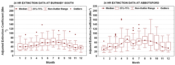
Seasonal variations in visibility at the urban-impacted sites in the WISE were analyzed by So et al. (2013). Figure 9.1a shows measured (observed) extinction at Burnaby South and Abbotsford. At both sites, the observed median extinction is statistically higher (p<0.1) during the fall, compared to spring and summer for the six year period (2003-2010). Higher frequencies of poor visibility days, as indicated by the upper non-outlier range and outliers, were observed from September to February at both sites. Observed extinction, however, is influenced by relative humidity (RH) and boundary layer height, among other meteorological factors. To remove the influence of RH and boundary layer height, the data were filtered for high RH conditions (>80%) and were seasonally adjusted for boundary layer height, as shown in Figure 9.1b. Based on adjusted extinction, the poorest visibility in the WISE occurred from May to September and best during the winter months. While the adjusted values do not reflect actual visibility conditions, they give an indication of the impact of anthropogenic pollutants on visibility. McKendry (2000) has also found that episodes of poor visibility in the Lower Fraser Valley often occur during the summer, following a period of elevated ozone.
Figure 9.1. Seasonal 24-hour aerosol reconstructed extinction in the Lower Fraser Valley (2003 - 2010).
(a) Observed Extinction
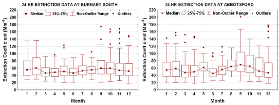
(b) Meteorologically Adjusted Extinction
Notes: Observed extinction were reconstructed using the revised IMPROVE formula (Pitchford, 2007). 24-hour PM2.5speciation data, 1-in-3 day sampling for the years 2003-2010 (NAPS Stations 100119, 101004). (So et al., 2013)
Description of Figure 9.1
Figure 9.1 is composed of four box-plots showing the median, 25-75% range, full non-outlier range, and outliers for 24hr extinction in the Lower Fraser Valley. The upper two plots show observed extinction coefficient in Mm-1as a function of month for Burnaby South and Abbotsford. The bottom two plots show meteorologically adjusted extinction coefficient in Mm-1 as a function of month for Burnaby South and Abbotsford. There is a note that observed extinctions were reconstructed using the revised IMPROVE formula (Pitchford, 2007), 24-hour PM2.5 speciation data, and 1-in-3 day sampling for the years 2003-2010 (NAPS Stations 100119, 101004). (So et al., 2013)
For Burnaby South the observed extinction data (all in Mm-1) are as follows.
- January: median 55, 25-75% range 40-80, full non-outlier range 30-140.
- February: median 60, 25-75% range 40-90, full non-outlier range 30-138.
- March: median 45, 25-75% range 40-60, full non-outlier range 25-95.
- April: median 45, 25-75% range 40-60, full non-outlier range 25-95, one outlier at 99.
- May: median 50, 25-75% range 40-65, full non-outlier range 20-85, outliers at 118 and 122.
- June: median 45, 25-75% range 40-60, full non-outlier range 20-85.
- July: median 50, 25-75% range 40-65, full non-outlier range 35-100.
- August: median 55, 25-75% range 45-60, full non-outlier range 25-90, one outlier at 105.
- September: median 60, 25-75% range 45-80, full non-outlier range 20-125, outliers at 140 and 175.
- October: median 60, 25-75% range 45-75, full non-outlier range 20-120, outliers at 125, 160, and 170.
- November: median 55, 25-75% range 40-75, full non-outlier range 25-115, outliers at 130, 140, 158, 160 and 170.
- December: median 55, 25-75% range 40-75, full non-outlier range 18-122, outliers at 145 and 150.
For Abbotsford the observed extinction data (all in Mm-1) are as follows.
- January: median 55, 25-75% range 35-75, full non-outlier range 20-130, one outlier at 140.
- February: median 60, 25-75% range 35-75, full non-outlier range 22-130, outliers at 150 and 160.
- March: median 45, 25-75% range 40-70, full non-outlier range 20-105, outlier at 130 and 150.
- April: median 45, 25-75% range 40-65, full non-outlier range 15-115, outliers at 145 and 150.
- May: median 60, 25-75% range 55-80, full non-outlier range 20-100, one outlier at 120.
- June: median 45, 25-75% range 38-58, full non-outlier range 25-85, one outlier at 118.
- July: median 58, 25-75% range 42-65, full non-outlier range 25-95, outliers at 105 and 120.
- August: median 60, 25-75% range 55-82, full non-outlier range 35-118.
- September: median 65, 25-75% range 50-102, full non-outlier range 25-170, one outliers at 200.
- October: median 62, 25-75% range 50-98, full non-outlier range 22-140.
- November: median 50, 25-75% range 38-90, full non-outlier range 22-122.
- December: median 45, 25-75% range 35-75, full non-outlier range 18-120, outliers at 142, 160, 175, and 180.
For Burnaby South the meteorologically adjusted extinction data (all in Mm-1) are as follows.
- January: median 40, 25-75% range 25-55, full non-outlier range 22-85.
- February: median 40, 25-75% range 30-52, full non-outlier range 25-75, one outlier at 95.
- March: median 42, 25-75% range 35-60, full non-outlier range 25-80.
- April: median 45, 25-75% range 38-60, full non-outlier range 25-90, one outlier at 105.
- May: median 55, 25-75% range 45-78, full non-outlier range 25-100, one outlier at 140.
- June: median 55, 25-75% range 45-75, full non-outlier range 25-110.
- July: median 60, 25-75% range 45-80, full non-outlier range 38-115.
- August: median 58, 25-75% range 45-70, full non-outlier range 30-95, one outlier at 110.
- September: median 55, 25-75% range 40-70, full non-outlier range 30-110.
- October: median 45, 25-75% range 35-55, full non-outlier range 20-70, one outlier at 105.
- November: median 38, 25-75% range 30-50, full non-outlier range 20-70, one outlier at 95.
- December: median 38, 25-75% range 30-50, full non-outlier range 20-70.
For Abbotsford the meteorologically adjusted extinction data (all in Mm-1) are as follows.
- January: median 30, 25-75% range 25-40, full non-outlier range 15-50, one outlier at 65.
- February: median 40, 25-75% range 30-55, full non-outlier range 15-90.
- March: median 40, 25-75% range 35-55, full non-outlier range 20-85, outliers at 90, 95, and 100.
- April: median 55, 25-75% range 40-80, full non-outlier range 20-125, outliers at 160 and 165.
- May: median 75, 25-75% range 60-90, full non-outlier range 22-120.
- June: median 55, 25-75% range 45-70, full non-outlier range 30-100, outliers at 115 and 125.
- July: median 70, 25-75% range 50-75, full non-outlier range 30-110, outliers at 120 and 140.
- August: median 72, 25-75% range 55-85, full non-outlier range 38-122.
- September: median 70, 25-75% range 50-98, full non-outlier range 22-160.
- October: median 60, 25-75% range 30-90, full non-outlier range 22-130.
- November: median 40, 25-75% range 25-60, full non-outlier range 20-90.
- December: median 38, 25-75% range 25-60, full non-outlier range 18-92.
At the urban Beacon Hill site in Seattle (Figure 9.2 a), observed (unadjusted) median extinction was statistically higher (p<0.05) during the fall months compared to the spring and summer for the period 2001 to 2011. The occurrences of poor visibility conditions, as indicated by the upper non-outlier range and outliers, were more frequent from September to February. At this site, smoke from wood burning may play a role during the colder months and/or it may be attributable to increased humidity and condensation of semi-volatiles due to the cooler temperatures and reduced boundary layer heights. Observations from the more rural Mount Rainier site show the opposite pattern (Figure 9.2 b), with a statistically higher (p<0.05) median extinction during the summer compared to all other seasons. The seasonal pattern at Mount Rainier may be related to a combination of smoke from forest fires and biogenic secondary organic particulate formation. In addition, as the Mount Rainier site is situated at an elevation of 439 m, the effects of boundary layer height on extinction during winter time may not be as significant as those at lower elevation sites.
Figure 9.2. Seasonal 24-hour reconstructed extinction in the Puget Sound (2000-2011).
(a) Beacon Hill*
(b) Mount Rainier
Notes: 24-hour speciation data, 1-in-3 day sampling for the years 2001-2011 at Beacon Hill* (IMPROVE site: 53-033-0080) and for the period 2000-2011 at Mount Rainier (IMPROVE site: 53-053-0014).
Description of Figure 9.2
Figure 9.2 is composed of two box-plots showing the median, 25-75% range, full non-outlier range, and outliers for 24hr reconstructed extinction in Puget Sound. The left plot shows total extinction in Mm-1 for Beacon Hill and the right plot shows total extinction in Mm-1 for Mount Rainier. There is a note that the plots are from 24-hour speciation data, 1-in-3 day sampling for the years 2001-2011 at Beacon Hill* (IMPROVE site: 53-033-0080) and for the period 2000-2011 at Mount Rainier (IMPROVE site: 53-053-0014).
For Beacon Hill the total extinction data (all in Mm-1) are as follows.
- January: median 60, 25-75% range 40-90, full non-outlier range 20-160, outliers at 170,195, and 210.
- February: median 60, 25-75% range 40-105, full non-outlier range 20-195, outliers at 220, and 230.
- March: median 50, 25-75% range 35-65, full non-outlier range 20-100, outliers at 110, 130,140,and 145.
- April: median 50, 25-75% range 40-70, full non-outlier range 25-110, outliers at 120, and 135.
- May: median 55, 25-75% range 40-70, full non-outlier range 25-110.
- June: median 50, 25-75% range 38-65, full non-outlier range 20-90, outliers at 125.
- July: median 55, 25-75% range 45-70, full non-outlier range 25-110, outliers at 115,120, and 145.
- August: median 60, 25-75% range 50-75, full non-outlier range 25-120, outliers at 145.
- September: median 65, 25-75% range 55-85, full non-outlier range 25-120, outliers at 140, 145 and 150.
- October: median 80, 25-75% range 55-105, full non-outlier range 25-185, outliers at 230,235,250,255, and 265.
- November: median 65, 25-75% range 50-100, full non-outlier range 25-175, outliers at 180,185,225 and 235.
- December: median 60, 25-75% range 45-105, full non-outlier range 25-200, outliers at 220, and 230.
For Mount Rainier the total extinction data (all in Mm-1) are as follows.
- January: median 20, 25-75% range 15-25, full non-outlier range 10-35, several outliers from 38 to 50.
- February: median 25, 25-75% range 20-30, full non-outlier range 10-50.
- March: median 25, 25-75% range 20-30, full non-outlier range 10-55, several outliers from 58-70.
- April: median 30, 25-75% range 25-40, full non-outlier range 10-60, outliers at 68, 70, 75 and 80.
- May: median 30, 25-75% range 25-45, full non-outlier range 10, outliers at 85.
- June: median 30, 25-75% range 25-50, full non-outlier range 10-80.
- July: median 40, 25-75% range 35-58, full non-outlier range 20-90, several outliers from 90 to110.
- August: median 45, 25-75% range 35-55, full non-outlier range 15-75.
- September: median 40, 25-75% range 30-50, full non-outlier range 15-75, outliers at 80, 95 and 100.
- October: median 35, 25-75% range 30-45, full non-outlier range 10-70, outliers at 75 and 85.
- November: median 25, 25-75% range 20-30, full non-outlier range 10-50, several outliers from 55 to 65.
- December: median 20, 25-75% range 20-28, full non-outlier range 10-40 several outliers from 45 to 50.
Hourly Reconstructed Light Extinction Measurements
In addition to reconstructing extinction using PM measurements, light extinction can be reconstructed from optical measurements from an ambient nephelometer (bscat), NO2 analyzer (bag) and aethalometer (bap). Using this method, the median hourly extinction was calculated to be 51 Mm-1 and 46 Mm-1 (visual range of 77 km and 85 km) for Chilliwack and Vancouver Airport, respectively, in 2011 (So et al., 2013). The highest median extinction occurred in the August to December period at both Chilliwack and Vancouver Airport (Figure 9.3). It should be noted that the observed trend is based on one year of data only, where high extinction events can potentially skew the seasonal pattern. The best visibility (lowest median extinction) occurred from January to April in Chilliwack and from February to April at Vancouver Airport (So et al., 2013).
Figure 9.3. Seasonal hourly extinction reconstructed from optical measurements in the Lower Fraser Valley.

Notes: Extinction was estimated using optical measurements from ambient nephelometer (bscat), aethalometer (bap), and NO2 analyzer (bag)
Description of Figure 9.3
Figure 9.3 is composed of two box-plots showing the median, 25-75% range, and full non-outlier range for seasonal hourly extinction reconstructed from optical measurements in the Lower Fraser Valley. The left plot shows hourly bext in Mm-1 for Chilliwack from Jan 1, 2011 to Dec 31, 2011 and the right plot shows hourly bext in Mm-1 for Vancouver airport from Feb 11, 2011 to Dec 31, 2011. There is a note that extinction was estimated using optical measurements from ambient nephelometer (bscat), aethalometer (bap), and NO2 analyzer (bag).
For Chilliwack the hourly bext data (all in Mm-1) are as follows.
- January: median 38, 25-75% range 25-70, full non-outlier range 10-135.
- February: median 38, 25-75% range 25-55, full non-outlier range 10-100.
- March: median 38, 25-75% range 25-50, full non-outlier range 15-90.
- April: median 40, 25-75% range 30-50, full non-outlier range 20-90.
- May: median 50, 25-75% range 35-70, full non-outlier range 15-120.
- June: median 45, 25-75% range 30-65, full non-outlier range 15-122.
- July: median 42, 25-75% range 30-60, full non-outlier range 15-100.
- August: median 70, 25-75% range 50-90, full non-outlier range 25-150.
- September: median 60, 25-75% range 35-90, full non-outlier range 15-165.
- October: median 70, 25-75% range 45-110, full non-outlier range 25-190.
- November: median 55, 25-75% range 35-80, full non-outlier range 15-155.
- December: median 60, 25-75% range 40-120, full non-outlier range 15-235.
For Vancouver airport the hourly bext data (all in Mm-1) are as follows.
- February: median 35, 25-75% range 28-48, full non-outlier range 15-75.
- March: median 35, 25-75% range 28-50, full non-outlier range 10-85.
- April: median 40, 25-75% range 28-55, full non-outlier range 15-95.
- May: median 45, 25-75% range 32-60, full non-outlier range 18-100.
- June: median 42, 25-75% range 30-65, full non-outlier range 15-110.
- July: median 40, 25-75% range 30-50, full non-outlier range 18-90.
- August: median 50, 25-75% range 38-65, full non-outlier range 20-110.
- September: median 50, 25-75% range 40-70, full non-outlier range 15-115.
- October: median 55, 25-75% range 38-80, full non-outlier range 22-145.
- November: median 55, 25-75% range 38-75, full non-outlier range 20-130.
- December: median 65, 25-75% range 45-100, full non-outlier range 18-185.
Figure 9.4. Diurnal light extinction reconstructed from hourly optical measurements at Abbotsford.
(a) Observed Extinction
(b) Meteorologically Adjusted Extinction
Notes: Extinction was estimated using optical measurements from ambient nephelometer (bscat), aethalometer (bap), and NO2 analyzer (bag).
Description of Figure 9.4
Figure 9.4 is composed of two box-plots showing the median, 25-75% range, and 1-99% range for Abbotsford. The left plot shows observed extinction and the right shows the meteorologically adjusted extinction (RH and mixing height adjusted data). There is a note that extinction was estimated using optical measurements from ambient nephelometer (bscat), aethalometer (bap), and NO2 analyzer (bag).
For the observed extinction plot diurnal bext (in Mm-1) is given as the sum of bscat (from a nephelometer), bap (from an aethalometer), and bag(from an NO2 analyzer). The data is for the period from May 28, 2009 through March 31, 2010. At 0000hrs the median value is approximately 60 Mm-1, it remains at this level through 0300hrs after which point it declines steadily to a minimum of just below 40 Mm-1 at 1400hrs. It then rises steadily to a maximum of just over 60 Mm-1at 2100hrs before declining slightly to 60 Mm-1 at 2400hrs. The 25% value remains between 35 and 40 Mm-1until after 0900hrs, it then drops to approximately 30 Mm-1 through 1800hrs before rising back to 35-40 Mm-1. The 75% value is approximately 95 Mm-1from 0000hrs to 0300hrs then declines steadily to a minimum of approximately 55 Mm-1 at 1500hrs before rising back to just below 100 Mm-1 at 2400hrs. The 1% value remains between 10 and 20 Mm-1 throughout the day. The 99% value is approximately 250 Mm-1 at 0000hrs, it drops to below 200 Mm-1 at 0100 hrs before rising back up to around 220 Mm-1 from 0200 through 0500hrs. It declines steadily to a minimum of 110 Mm-1at 1400hrs with the exception of 0800hrs where it spikes up to 220 Mm-1. After 1400hrs it rises steadily to 220 Mm-1 at 2400hrs.
For the meteorologically adjusted extinction plot diurnal bext (in Mm-1) is also given as the sum of bscat (from a nephelometer), bap (from an aethalometer), and bag(from an NO2 analyzer). The data is for the period from May 28, 2009 through March 31, 2010. At 0000hrs the median bext is approxiamteky 25 Mm-1, this declines to a minimum of 20 Mm-1at 0400hrs before rising steadily to just below 60 Mm-1at 1000hrs. from 1000 to 1300hrs it rises very slightly to a maximum of approximately 60 Mm-1. After 1300hrs it declines steadily to 25 Mm-1 at 2400hrs. The 25% value follows a similar pattern falling from just below 20 Mm-1 to approximately 10 Mm-1 at 0400hrs before rising to just above 40 Mm-1 at 1300hrs and falling to 20 Mm-1 at 2400hrs. The 75% value follows the same pattern starting at 40 Mm-1, falling to approximately 30 Mm-1, rising to just over 80 Mm-1, and then falling to approximately 50 Mm-1. The 1% value also follows the same pattern starting at 10 Mm-1, falling to approximately 5 Mm-1, rising to just over 25 Mm-1, and then falling to approximately 10 Mm-1. The 99% value is approximately 145 Mm-1 at 0000hrs, falls to 70 Mm-1 at 0600hrs, and rises to 200 Mm-1 at 1300hrs. Spikes to 190 Mm-1 and 210 Mm-1occur at 0800 and 1100 hrs respectively. After 1300hrs the value falls to just over 100 Mm-1 at 2100hrs before rising to 125 Mm-1 at 2400hrs.
The diurnal pattern of visibility, as inferred from reconstructed extinction for the period May 2009 to April 2010 at Abbotsford (Figure 9.4 a), indicates that observed extinction is lowest between 14 and 15 hrs local time and highest during the night between 21 hrs and 4 in the morning. During daytime hours, observed extinction declines as the day progresses and then increases again after 16 hrs. After meteorological adjustment for RH and boundary layer height (Figure 9.4 b), the diurnal pattern of extinction reveals a maximum during daylight hours and a minimum during the night.
9.2.2 Visibility Perception
While there is currently no standard for visibility, impairment can be assessed relative to natural visibility conditions and relative to perceived acceptability. The term “natural visibility conditions” represents the long-term degree of visibility that is estimated to exist in a given mandatory Federal Class I area in the absence of anthropogenic impairment (U.S. EPA, 2003). Under the U.S. Regional Haze Rule, Mount Rainier has an estimated natural visual range of 180 km (worst days) to 300 km (best days) (WA DOE, 2002). Based on ambient measurements, the observed mean visual range in 2008 was approximately 150 km. For all 1-in-3 day observations since 2001, Mt Rainier’s visual range exceeded 180 km 31% of the time, and 300 km 2.5% of the time.
Based on an assessment of visibility images taken at several locations in the LFV, visibility impairment in the WISE becomes noticeable at hourly PM2.5concentrations as low as 8-10 μg/m3. At concentrations between 10-20 μg/m3 visibility is significantly affected, while above 20 μg/m3 it is severely affected, often completely obscuring views of surrounding mountain ranges (Vingarzan, 2010).
The development of a visibility goal is currently underway in the Georgia Basin, led by the British Columbia Visibility Coordinating Committee (BCVCC, 2013). As part of this effort, a recent study in the Lower Fraser Valley quantified levels of acceptable visibility using a set of Visual Air Quality (VAQ) ratings and developed a corresponding visibility index to assess visibility impairment for a scene in Chilliwack with visual targets ranging from 15-45 km from the observer (Sakiyama and Kellerhals, 2010). According to the VAQ-based visibility index, the Chilliwack site (Figure 9.5) experienced very poor and poor visibility from 0% to 5% of the time, fair visibility 25%, good visibility 43% and excellent visibility 26% of the time in 2011. At Chilliwack the greatest number of poor and very poor hourly visibility observations during daylight hours occurred in the fall (Vingarzan, 2010). Additional work is currently underway to further develop and validate the proposed visibility index.
Figure 9.5. 2011 annual distribution of visibility perception at Chilliwack based on visibility index categories developed by Sakiyama and Kellerhals (2010).
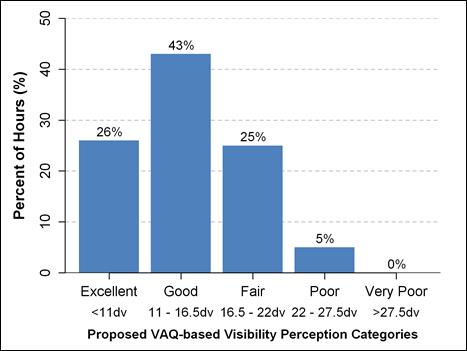
Notes: Hourly deciview observations were calculated using measurements from ambient nephelometer (bscat), aethalometer (bap), and NO2 analyzer (bag) collected at Chilliwack in 2011. Percentages indicate the distribution of visibility across each of the visibility index categories (So et al., 2013). Note that the proposed visibility index only applies to daytime hours (sunrise + 2 hrs ≤ hours ≤ sunset - 2 hrs) when RH ≤ 75%. The assessed scene consisted of visual targets ranging from 15 to 45 km from the observer.
Description of Figure 9.5
Figure 9.5 is a bar chart showing the percent of hours in each of the five proposed VAQ-based visibility perception categories. The categories are very poor (>27.5 deciviews), poor (22-27.5 deciviews), fair (16.5- 22 deciviews), good (11-16.5 deciviews), and excellent (<11 deciviews). There is a note that hourly deciview observations were calculated using measurements from ambient nephelometer (bscat), aethalometer (bap), and NO2 analyzer (bag) collected at Chilliwack in 2011. The percentages in each category are very poor 0%, poor 5%, fair 25%, good 43%, and excellent 26%. There is a note that percentages indicate the distribution of visibility across each of the visibility index categories (So et al., 2013). Note that the proposed visibility index only applies to daytime hours (sunrise + 2 hrs ≤ hours ≤ sunset - 2 hrs) and when RH ≤ 75%. The assessed scene consisted of visual targets ranging from 15 to 45 km from the observer.
Another study conducted locally by Environment Canada evaluated WISEresidents’ perceived violation ratings in relation to frequency of poor visibility days (in addition to severity of a single day). Focus groups consisting of local area residents were presented with a series of photographic images depicting 10 day poor visibility scenarios of regional vistas. The study was undertaken to gain an understanding of how respondents respond to multi-day visibility scenarios and whether the policy implications would be similar to those derived from the previous one day event studies. The results indicated that people respond most favourably to visibility improvements that resulted in a greater number of days in the best category. A policy that simply removed the very bad days, without a corresponding increase in the very best days, would have little effect. The study recommended that a visibility standard should specify a minimum number of good (best quintile) visibility days over the year (McNeill and Roberge, 2007).
9.2.3 Visibility Trends
Given the decreasing trends in PM2.5 concentrations in the Georgia Basin/Puget Sound airshed, it is reasonable to expect average visibility to be improving. This appears to be supported by a review of long-term visibility observations.
Visibility Trends in the Puget Sound
The daily average visual range at Mount Rainier has improved over the past 20 years, according to the trend presented in Figure 9.6. The 12-month visual range moving average increased from about 100 km in the late 1980s to over 150 km in 2008. Most of the year-to-year variability at Mount Rainier is explained by meteorological conditions, whereas the underlying trend is likely the result of emission reductions.
Figure 9.6. Visibility Trends at Mount Rainier (1987-2008)
Notes: Data are the daily average visibility at Mt Rainier, measured on a 1 in 3 day cycle, from the IMPROVE network MORA site.
Description of Figure 9.6
Figure 9.6 is a plot of visual range in km as a function of year for Mount Rainier from 1987 through 2008. The raw visual range is plotted in addition to the 12-month moving average. There is a note that the data are the daily average visibility at Mt Rainier, measured on a 1 in 3 day cycle, from the IMPROVE network MORA site. The 12-month moving average increased steadily from about 100 km in 1987 to over 150 km in 2008. Small fluctuations in the moving average occurred on a scale of ± 5-10km. The non-averaged data is considerably noisier, covering a range of approximately ± 100km.
A Washington Department of Environment analysis (WA DOE, 2002) of extinction data from Mount Rainier from 1988-1999 found statistically significant decreasing trends in extinction on the best days, worst days and all days. A visibility loss attribution analysis of these data showed that all components were statistically decreasing except soil, with organic and elemental carbon showing the greatest improvements. Visibility loss attribution is discussed further in the next section.
The improvement at Mount Rainier corresponds with the improvement in average visual range in the Puget Sound airshed. The 12-month visual range moving average measured at nephelometer sites in the Puget Sound’s region monitoring network has steadily increased from about 80 km in 1990 to about 130 km in 2009 (PSCAA, 2009).
Visibility Trends in the Georgia Basin
As with PM2.5, the period of record of extinction measurements in the Georgia Basin (which started in 2003) is too short to establish robust trends. However, a long term trend analysis of observer-based visibility records from Vancouver and Abbotsford international airports for the period 1953-2006 (So and Vingarzan, 2010) indicate that visibility ≥24.1 km increased sharply after 1970, while the trend in smoke and haze declined steadily since 1960. These improvements parallel the introduction of air quality regulations, the displacement of heavy industry and changes in home heating fuel.
9.3 Visibility Loss Attribution
Understanding the underlying causes of poor visibility requires attribution analysis of visibility loss, which is similar to conducting a compositional analysis of PM. Recent attribution analyses of extinction were performed for the Burnaby and Abbotsford sites in the Georgia Basin and for Mount Rainier in the Puget Sound.
9.3.1 Visibility Loss Attribution in the Georgia Basin
Figure 9.7 summarizes the extinction attribution analysis performed for Burnaby South and Abbotsford in the Lower Fraser Valley (So et al., 2013). At Burnaby South, both organic matter and nitrate accounts for the largest portion of visibility loss (21% each) followed by elemental carbon (20%), sulphate (17%), and NO2 (11%). At Abbotsford, nitrate accounts for a slightly larger proportion of visibility loss (30%) followed by organic matter (23%), elemental carbon (17%), sulphate (15%) and coarse mass (7%).
Figure 9.7. Annual contributions to total reconstructed extinction by particle and gas species at Burnaby South and Abbotsford for 2003-2010.
Notes: Rayleigh scattering (which accounts for approximately 20% of total extinction) is not included;
SO4 = sulphate; NO3 = nitrate; OM = organic matter; EC = elemental carbon; Soil = fine soil;
SS = sea salt; NO2= nitrogen dioxide; CM=coarse mass
Description of Figure 9.7
Figure 9.7 is composed of two pie charts, one showing the annual contributions to total reconstructed extinction by particle and gas species at Burnaby South and one showing the annual contributions to total reconstructed extinction by particle and gas species at Abbotsford. There is a note that Rayleigh scattering (which accounts for approximately 20% of total extinction) is not included.
For Burnaby South the contributions are as follows. Sulphate 17%, nitrate 21%, organic matter 21%, elemental carbon 20%, fine soil 1%, sea salt 2%, nitrogen dioxide 11%, and coarse mass 7%.
For Abbotsford the contributions are as follows. Sulphate 15%, nitrate 30%, organic matter 23%, elemental carbon 17%, fine soil 1%, sea salt 2%, nitrogen dioxide 5%, and coarse mass 7%.
So et al. (2013) also studied the seasonal variability in extinction attribution for the WISE (not shown). They found that nitrate accounts for a larger percentage of extinction during the fall and winter and sulphate accounts for a larger percentage during the summer. An analysis on the meteorologically-adjusted worst 20% visibility conditions (Figure 9.8) revealed significant contributions from organic matter at both Burnaby South and Abbotsford. At Abbotsford, the worst visibility days were also significantly impaired by nitrate.
Figure 9.8. Contributions to RH filtered and boundary layer height adjusted extinction by particle and gas species for the best and worst 20% visibility conditions at Burnaby South and Abbotsford (2003 - 2010).
Note: Rayleigh scattering (which accounts for approximately 20% of total extinction) is not included SO4 = sulphate; NO3 = nitrate; OM = organic matter; EC = elemental carbon; Soil = fine soil; SS = sea salt; NO2 = nitrogen dioxide; CM=coarse mass
Description of Figure 9.8
Figure 9.8 shows the contribution to adjusted extinction (in Mm-1) by 8 different particle and gas species for the best and worst 20% visibility conditions at Burnaby South and Abbotsford. The figure has a note that Rayleigh scattering (which accounts for approximately 20% of total extinction) is not included in the analysis.
For Burnaby South best 20% visibility the contributions to adjusted extinction are as follows. Sulphate 3 Mm-1; nitrate 3 Mm-1; organic matter 3 Mm-1; elemental carbon 4 Mm-1; fine soil <1 Mm-1; sea salt 1 Mm-1; nitrogen dioxide 3 Mm-1; and coarse mass 2 Mm-1.
For Burnaby South worst 20% visibility the contributions to adjusted extinction are as follows. Sulphate 12 Mm-1; nitrate 11 Mm-1; organic matter 20 Mm-1; elemental carbon 13 Mm-1; fine soil 1 Mm-1; sea salt 1 Mm-1; nitrogen dioxide 8 Mm-1; and coarse mass 6 Mm-1.
For Abbotsford best 20% visibility the contributions to adjusted extinction are as follows. Sulphate 2 Mm-1; nitrate 2 Mm-1; organic matter 4 Mm-1; elemental carbon 4 Mm-1; fine soil <1 Mm-1; sea salt 1 Mm-1; nitrogen dioxide 2 Mm-1; and coarse mass 2 Mm-1.
For Abbotsford worst 20% visibility the contributions to adjusted extinction are as follows. Sulphate 12 Mm-1; nitrate 27 Mm-1; organic matter 24 Mm-1; elemental carbon 15 Mm-1; fine soil 1 Mm-1; sea salt 1 Mm-1; nitrogen dioxide 3 Mm-1; and coarse mass 6 Mm-1.
9.3.2 Visibility Loss Attribution in the Puget Sound
In Figure 9.9, extinction attribution data from Mount Rainier clearly shows the dominance of sulphate and organic matter during poor or worst-case visibility days. The data also show a significant reduction in light attenuation due to these two species, indicating that much of the visibility improvement seen in Figure 9.6 can be attributed to declines in sulphate and organic matter.
Figure 9.9. Mt. Rainier bextpollutant species trends for the 20% worst visibility days (IMPROVE)
Notes: ”IQR” (blue box) is defined as the inter-quartile range; outliers are not necessarily statistically significant
Description of Figure 9.9
Figure 9.9 is a plot of the light extinction (in Mm-1) attributed to each of seven pollutant species as a function of time. The y-axis shows light extinction in Mm-1 and the x-axis shows the years from 1988 to 2006. There is a note that data are the yearly average extinction for the 20% worst visibility days. Data for 1990 and 2003 are missing due to the site not meeting data completeness standards for those years.
Extinction attributed to ammonium sulphate was stable around 35 Mm-1 from 1989 through 1994. After 1994 there was a decline to approximately 22 Mm-1 in 1996 followed by a rise back to approximately 35 Mm-1 in 1998. There was then a decline to approximately 20 Mm-1 by 2002. In 2004 levels were around 22 Mm-1, this dipped to approximately 15 Mm-1 in 2005 before rising to approximately 22 Mm-1 in 2006.
Extinction attributed to organic matter declined fairly steadily from around 30 Mm-1 in 1989 to approximately 17 Mm-1 in 1995. The level rose to just below 25 Mm-1 in 1996 and remained between 20 and 25 Mm-1 until 1999. In 2000 the level dropped to approximately 15 Mm-1 and remained between 10 and 15 Mm-1 through 2002. In 2004 the level was just below 20 Mm-1 and it declined steadily to approximately 15 Mm-1 in 2006.
Extinction attributed to elemental carbon declined steadily from around 10 Mm-1 in 1989 to just above 5 Mm-1in 2006.
Extinction attributed to ammonium nitrate remained around 5 Mm-1 from 1989 through 2006.
Extinction attributed to coarse mass declined slightly from around 5 Mm-1 in 1989 to around 2.5 Mm-1 in 2006.
Extinction attributed to both soil and sea salt remained stable at around 1 Mm-1 from 1989 through 2006.
9.4 Emission Reductions and Regional Haze
Understanding the effects of emission reductions on regional haze is a necessary step in the development of policies aimed at improving regional visibility policy development. Reductions in emissions of most primary pollutants usually results in a reduction of regional haze; however, due to the non-linear nature of atmospheric chemistry, achieving these reductions may not be straight forward. Table 9.1 summarizes the effects of reductions of various atmospheric air pollutants on regional haze.
Table 9.1 Effects of reductions in secondary PM precursors and primary PM on regional haze (NARSTO, 2004).
|
Reduction in Pollutant Emissions
|
Change in Regional Haze
|
|
SO
2
|
decrease
|
|
NO
X
|
Possible small increase or decrease
1
|
|
VOC
|
Possible small increase or decrease
2
|
|
NH
3
|
decrease
|
|
Black Carbon
|
decrease
|
|
Primary Organic Compounds
|
decrease
|
|
Other Primary PM (Crustal and Metals, etc.)
|
decrease
|
Notes: Direction of the arrow indicates an increase or a decrease; blue is a desirable change and red is undesirable; size of the arrow indicates magnitude of the change. Small arrows signify possible or small change.
1 due to effect of NOx on oxidant levels (OH, H2O2, and O3) resulting in an increase in ammonium sulphate
2 due to less organic nitrogen compound formation and more OH available to form nitric acid
3 if airshed is NH3-limited
9.5 Modelling Visibility Impairment for the U.S. Regional Haze Rule
The 1977 Amendments to the U.S. Clean Air Act (CAA) set forth a program for protecting visibility in the nation’s national parks and wilderness areas (referred to hereafter as Class I areas). This section of the CAA establishes as a national goal the “…prevention of any future, and the remedying of any existing, impairment of visibility in mandatory Class I Federal areas which impairment results from man-made air pollution.” In 1999 EPA promulgated the Regional Haze Rule (RHR) to address regional haze. The RHR established the goal of achieving “natural” visibility conditions in all 156 federal Class I areas by 2064 (U.S. EPA, 1999). The four Class I areas in the Georgia Basin/Puget Sound (GB-PS) airshed are, from south to north, Mount Rainier National Park, Alpine Lakes Wilderness Area, Olympic National Park and North Cascades National Park.
Because the pollutants that lead to regional haze can originate from sources located across broad geographic areas, EPA encouraged the States and Tribes across the United States to address visibility impairment from a regional perspective. To assist States and Tribes in this effort, EPA funded five regional planning organizations (RPOs) to address regional haze and related issues. One of the main objectives of the RPOs is to analyze available data and conduct pollutant transport modelling to assist the States and Tribes in developing their regional haze implementation plans (U.S. EPA, 2011). The Western Regional Air Partnership (WRAP) is the RPO that covers the four Class I areas in the Puget Sound airshed. From the period of 2000 to 2010 the WRAP funded over $20 million dollars in the development of meteorological modelling, emissions inventories, air quality modelling, and other technical and policy tools to assist western States and Tribes in this effort (WRAP, 2009a).
The RHR does not mandate specific visibility milestones or rates of progress but instead calls for States and Tribes to establish goals for 10-year milestone increments that provide for “reasonable progress” toward achieving natural visibility conditions over the 60-year period from 2004 - 2064. In setting Reasonable Progress Goals (RPGs) for each 10-year target, States and Tribes must provide for an improvement in visibility for the most impaired days over the 10-year period of the State Implementation Plan (SIP) or Tribal Implementation Plan (TIP) and ensure no degradation in visibility for the least impaired days over the same period (U.S. EPA, 2007).
According to the RHR, the first Regional Haze SIPs and TIPs must specify emissions controls and reasonable progress expected to be achieved between the 2000-04 baseline and 2018, for each federal Class I area. Towards this goal, the WRAP developed baseline 2000-04 and 2018 emissions inventories (discussed more fully in Chapter 5, “Emissions”), meteorological modelling representative of the baseline period, and air quality modelling for the baseline and 2018 planning scenarios for the Western U.S. The 2018 planning scenarios included all ‘on the books’ emissions improvements from existing and planned point, mobile, and area emissions reduction programs as well as expected growth from, for example, population increases (WRAP, 2007).
Figure 9.10(a-d) depicts visibility measurements, 2018 projections, and 2018 and 2064 natural conditions goals for Mount Rainier National Park, Alpine Lakes Wilderness Area, Olympic National Park, and North Cascades National Park, respectively. These figures depict visibility using the deciview metric, which is designed to change linearly with human perception of visibility change. The 2064 natural conditions goals for the four Class I areas are in a range of 8.4 to 8.5 deciviews.
Inspection of the plots in Figure 9.10shows that in the Puget Sound the 2005-09 measured rate of progress in visibility is better than the charted linear rate of progress, based on the natural conditions goals for 2064. However, the 2018 WRAP model projections in all cases are worse than the charted linear rate of progress. At this juncture, it is unclear if measured trends in visibility will continue along the better than linear rates of progress or if 2018 WRAP model projections are more accurate. Washington State’s Regional Haze SIP, which outlines its strategy to meet 2018 Reasonable Progress Goals, is currently under review by EPA at the time of writing.
Figure 9.10. Measured (2000-04 and 2005-09) and projected (2018) progress against natural conditions goals for 2064, for four Class I Areas in Puget Sound. (a) Mount Rainier NP (b) Alpine Lakes Wilderness (c) Olympic NP and (d) Glacier Peak, North Cascades NP (adapted from WRAP, 2009b).
(a)
(b)
(c)
(d)
Notes: Measured average 2000-04 worst 20% visibility days (purple horizontal bar), measured average 2005-09 progress on worst 20% visibility days (red horizontal bar), 2018 20% worst visibility days, based on air quality model projections (green square), 2064 natural conditions goals (blue diamonds), and charted linear rate of progress from 2004 to 2064 (blue linear sloping line).
Description of Figure 9-10
Each of the four panels in Figure 9.10 is a plot of visibility (in deciviews) as a function of year. Each plot has four components, a horizontal bar spanning the years 2000 to 2004 at the measured average worst 20% visibility days for these years, a second horizontal bar spanning the years 2005 to 2009 showing the measured average progress worst 20% visibility days for these years, a point at 2018 showing the projected 20% worst visibility days (based on air quality model projections), and a point the natural condition goal for 2064. The charted linear rate of progress from 2004 to 2064 is shown by a line connecting the 2000-2004 measured average to the 2064 natural conditions goal.
In panel A data for Mount Rainier National Park, WA Class 1 area, is shown. The 2000-2004 baseline average is at approximately 18 deciviews. The 2005-2009 progress average is at approximately 16 deciviews and falls below the line connecting the 2000-2004 measured average to the 2064 natural conditions goal. The projected 2018 (PRP18b) value is at approximately 17 deciviews and falls above the line connecting the 2000-2004 measured average to the 2064 natural conditions goal. The 2064 natural conditions goal is at 8.5 deciviews.
In panel B data for Alpine Lakes W, WA Class 1 area, is shown. The 2000-2004 baseline average is at approximately 18 deciviews. The 2005-2009 progress average is at approximately 16 deciviews and falls below the line connecting the 2000-2004 measured average to the 2064 natural conditions goal. The projected 2018 (PRP18b) value is at approximately 16 deciviews and falls above the line connecting the 2000-2004 measured average to the 2064 natural conditions goal. The 2064 natural conditions goal is at 8.4 deciviews.
In panel C data for Olympic National Park, WA Class 1 area, is shown. The 2000-2004 baseline average is at approximately 17 deciviews. The 2005-2009 progress average is at approximately 15 deciviews and falls below the line connecting the 2000-2004 measured average to the 2064 natural conditions goal. The projected 2018 (PRP18b) value is at approximately 16 deciviews and falls above the line connecting the 2000-2004 measured average to the 2064 natural conditions goal. The 2064 natural conditions goal is at 8.4 deciviews.
In panel D data for Glacier Peak W, WA:North Cascades, WA Class 1 area, is shown. The 2000-2004 baseline average is at approximately 16 deciviews. The 2005-2009 progress average is at approximately 13 deciviews and falls below the line connecting the 2000-2004 measured average to the 2064 natural conditions goal. The projected 2018 (PRP18b) value is at approximately 17 deciviews and falls above the line connecting the 2000-2004 measured average to the 2064 natural conditions goal. The 2064 natural conditions goal is at 8.4 deciviews.
9.6 Visibility Modelling in the Georgia Basin & Puget Sound
9.6.1 High Resolution Photochemical Modelling
The effects of emission reduction scenarios on visibility were examined by RWDI (2006) using the MC2-SMOKE-CMAQ modelling system at 4 km resolution. In the first scenario, the effects of a 60% reduction in ammonia emissions were examined relative to the business as usual scenario. Figure 9.1 presents an example of hourly model output for this scenario during stagnant meteorological conditions. On average, there was a modelled visibility improvement of 11% over the entire WISE for summer stagnant and summer mixed conditions relative to the base case (RWDI, 2006; Meyn and Vingarzan, 2008). Smaller improvements (<5%) were projected for the winter case.
Figure 9.11 CMAQ modelled differences in visibility (light extinction) between the 60% reduction in ammonia and the 2000 Base Case in the Lower Fraser Valley. Source: RWDI, 2006.
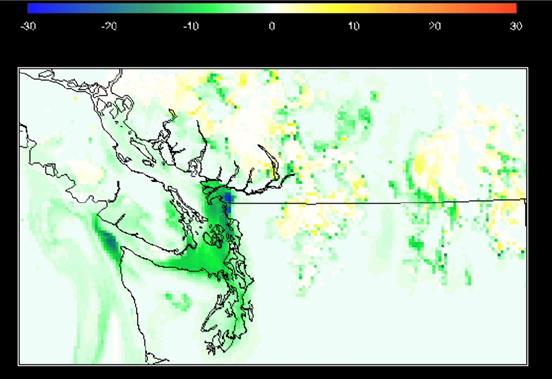
Notes: The scale is denoted in units of percent improvement in light extinction (bext). Values below zero indicate improvements in visibility. The image is a difference map showing changes in light extinction relative to the 2000 base case and represents hourly output from the August 13, 2001 run.
Description of Figure 9-11
Figure 9.11 is a line map of northern Washington and southern British Columbia colored to show percent improvement in light extinction (bext). Values below zero indicate improvements in visibility. The image is a difference map showing changes in light extinction relative to the 2000 base case and represents hourly output from the August 13, 2001 run.
There was an approximately 10% improvement in light extinction for most of Puget Sound, the eastern Strait of Juan de Fuca, the southern Strait of Georgia, the metro Vancouver area, and the Saanich Peninsula. The mouth of the Strait of Juan de Fuca had an approximately 10-20% improvement. The area just to the east of Boundary bay, spanning both sides of the border, showed an improvement of approximately 20%. The remainder of the airshed show improvements of 0 to 10%.
The second scenario involved modelling of the Metro Vancouver 2015 business-as-usual (BAU) scenario relative to the 2001 base case. This scenario resulted in a minor degradation of visibility in the WISE of 1.3% during summer stagnant conditions. The third scenario involved modelling of emission reductions associated with the adoption of Metro Vancouver’s 2015 Air Quality Management Plan (AQMP) (RWDI, 2006). This scenario resulted in visibility improvements of 2.6% for summertime stagnant conditions, 4.6% for summertime mixed conditions and 3.2% for winter conditions (RWDI, 2006; Meyn and Vingarzan, 2008). Note that for the 2015 BAU and Metro Vancouver AQMP scenarios, spatially averaged visibility changes were projected to be less than 1 deciview.
9.6.2 AURAMS Modelling
Air quality model simulations have been used to estimate future visibility across Canada using the regional air quality model AURAMS (see Chapter 10, Regional Air Quality Modelling for a more complete description). The effects of the implementation of Canada’s Clean Air Regulatory Agenda (CARA), which are expected to result in emission reductions of NOx, SO2, VOCs and primary PM2.5, have been modelled. Figure 9.12 illustrates the difference in annual average visibility between 2015 business-as-usual (BAU) and 2015 CARA emissions projection scenarios. The 2015 BAU scenario incorporates emissions projections that are based on Canadian and U.S. official projections and take into account growth and the implementation of regulations that have been promulgated and will be in place by 2015, including the U.S. Clean Air Interstate Rule (CAIR) but not the proposed Clean Air Regulatory Agenda (CARA) for Canada; the 2015 CARA scenario is identical but includes the proposed CARA emission reductions. It should be noted that CAIR is only applicable to some states in the eastern U.S. and any future emission projection based on CAIR for the western states should be used with caution. Nevertheless, it is assumed that this does not affect the differences between the 2015 BAU and 2015 CARA projections, as the same bias occurs in both scenarios.
Figure 9.12 AURAMS modelled differences in annual average visibility between the 2015 CARA and business-as-usual (2015 BAU) scenario. Source: Environment Canada, 2011.
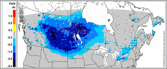
Description of Figure 9.12
Figure 9.12 is a line map of North America spanning from approximate 40°N to 65 °N. The map is colored by modelled differences in annual average visibility between the 2015 CARA and business-as-usual (2015 BAU) scenarios. The color scale is from -3.0 to 1.5 deciviews (dv). The most significant visibility improvements are seen in Alberta, Saskatchewan, Manitoba, the northern portions of Montana and North Dakota, southern Ontario, along the St Lawrence River and in some areas of the Maritimes. In these areas improvements of -0.2 to 3.0 dv are predicted. As stated in the text, visibility is expected to remain relatively similar for the Georgia Basin Puget Sound airshed (a modelled difference of -0.2 to 0.2 deciviews), with the exception of the Greater Vancouver area, where the annual average visibility would improve by 0.2 to 0.5 deciviews.
The model results project an improvement in visibility over central and western Canada under the 2015 CARA scenario, relative to the 2015 BAU scenario. This improvement is largely driven by emission reductions in electricity generation and base-metal smelting sectors (Bouchet and Buset, 2012). For the Georgia Basin Puget Sound airshed, visibility is expected to remain relatively similar (a modelled difference of -0.2 to 0.2 deciviews), with the exception of the Greater Vancouver area, where the annual average visibility would improve by 0.2 to 0.5 deciviews.
9.7 Chapter Summary
Visibility degradation and regional haze affect tourism and diminish the quality of life for residents. Visibility is commonly expressed in units of light extinction, deciviews or visual range. Visibility degradation varies seasonally and spatially depending on emissions and meteorology, with the worst days occurring in the summer on rural Mount Rainier (WA DOE, 2002) and in the fall in Seattle and at the urban-impacted Lower Fraser Valley sites. Seasonal and diurnal patterns of visibility are strongly affected by meteorological conditions, such as relative humidity and boundary layer height. After adjustment for these two factors, the seasonal pattern of visibility in the Lower Fraser Valley showed that impacts due to anthropogenic pollutants are higher in the summer and lower in the winter. At Class I Areas in the U.S. (National Parks and Wilderness Areas of a certain size), visibility is regulated under the U.S. Regional Haze Rule, which requires continuous improvement of worst days and protection of clear days until man-made degradation is eliminated by 2064 (WA DOE, 2003). Natural visibility at the Mount Rainier site is estimated to be 180 km on the worst days and over 300 km on the best days (WA DOE, 2002).
In the Georgia Basin, there is no regulatory imperative to control visibility, although the development of a visibility goal and management framework is underway through efforts of the BC Visibility Coordinating Committee. Based on the proposed WISE Visual Air Quality Index, an analysis of visibility data from Chilliwack in the eastern WISE indicated that in 2011, visibility was rated in the good category approximately half the time, and in the fair and excellent categories, approximately one quarter of the time, respectively.
Long-term trends show statistically significant improvements in visibility in both the Georgia Basin and the Puget Sound. At Mount Rainier, visibility improvement is associated with statistically significant decreases in ammonium sulphate and organic carbon.
Ambient visibility measurements for the four Class I areas in the Puget Sound are showing a better than that expected improving trend, when compared with model projections performed for the year 2018 by the Western Region Air Partnership (WRAP). It is unclear at present if measured trends in visibility will continue along the better than linear rates of progress or if 2018 model projections indicating improvements at a rate less than the charted linear rate of progress are more accurate.
CMAQmodelling featuring a hypothetical 60% reduction in ammonia showed a modest improvement in visibility for summertime stagnant and mixed conditions of 11%, relative to base case. With the implementation of a number of emission reductions under Metro Vancouver’s 2015 Air Quality Management Plan, visibility is projected to improve slightly (<5% over base case) for both summer and winter conditions. Note, however, that spatially averaged visibility changes resulting from implementation of Metro Vancouver AQMP scenario were projected to be relatively small (< 1 deciview).
The AURAMS model was applied on a continental scale to estimate the effects of Canada’s Clean Air Regulatory Agenda (CARA) on future visibility. While model results indicated improvements in central and some parts of western Canada, they also indicated that visibility conditions would remain relatively constant in the majority of the Georgia Basin/Puget Sound region, with the exception of the Greater Vancouver area, where visibility is expected to improve slightly. Modelling work currently underway will more specifically inform visibility management efforts in the Canadian Lower Fraser Valley.
The need to further improve and protect visibility is recognised by regional and federal agencies in both the Georgia Basin and Puget Sound. In British Columbia, the British Columbia Visibility Coordinating Committee is managing a multi-faceted visibility program aimed at improving visibility in the Canadian Lower Fraser, while in Washington State, compliance with the U.S. Regional Haze Rule ensures that progress is made towards protecting visibility in national parks and protected areas.
9.8 References
Bouchet, V., and Buset, K, 2012. “Chapter 6: Model scenarios and applications.” In: Canadian Smog Science Assessment. Volume 1. Atmospheric Science and Environmental Effects. Environment Canada and Health Canada.(Executive summary) (Full report available upon request) Environment Canada, Science and Technology Branch, 4905 Dufferin St, Downsview, Ontario, M3H 5T4
Environment Canada, 2011. Air Quality Model Applications Section, National Prediction Operations, Meteorological Service of Canada.
Hand, J.L. and Malm, W.C., 2007. Review of the IMPROVE equation for estimating ambient light extinction coefficients. Journal of Geographical Research 112, D16203, doi:10.1029/2007JD008484.
Hoff, R.M., Guise-Bagley, L., Moran, M., McDonald, K., Nejedly, A., Campbell, I., Pryor, S., Golestani, Y., Malm, W.,1997. Recent visibility measurements in Canada. Proceedings (CD-ROM), 90th Annual Meeting of the Air and Waste Management Association, Toronto, Canada, June 8-13.
Lowenthal, D.H. and Kumar, N., 2003. PM2.5 mass and light extinction reconstruction in IMPROVE, Journal of the Air & Waste Management Association 53: 1109-1120.
McDonald, K., 2011. “Chapter 11. Impact of SMOG on Visibility in Developed Regions of Canada.” In: Canadian Smog Science Assessment. Volume 1. Atmospheric Science and Environmental Effects. Environment Canada and Health Canada.(Executive summary) (Full report available upon request) Environment Canada, Science and Technology Branch, 4905 Dufferin St, Downsview, Ontario, M3H 5T4
McKendry, I.G., 2000. PM10 Levels in the Lower Fraser Valley, British Columbia, Canada: An Overview of Spatiotemporal Variations and Meteorological Controls. Journal of the Air & Waste Management Association 50: 443-445.
McNeill, R. and Roberge, A., 2007. Factors Affecting Acceptable Visibility in the Lower Mainland of British Columbia. Unpublished report. 77p. Environment Canada, Vancouver, BC.
Meyn, S and Vingarzan R., 2008. CMAQ Model Evaluation in the Lower Fraser Valley Including Management Scenario Impacts on Concentrations of PM2.5, O3 and Visibility. Environment Canada, Meteorological Services, #201-401 Burrard, Vancouver, BC, V6S 3S5
NARSTO, 2004. Particulate Matter Science for Policy Makers: A NARSTO Assessment. P. McMurry, M. Shepherd, and J. Vickery, eds. Cambridge University Press, Cambridge, England. ISBN 0 52 184287 5.
Pitchford, M., and Malm, W.C., 1994. Development and application of a standard visual index. Atmospheric Environment 28: 1049-1054.
Pitchford, J., Malm, W., Schichtel, B., Kumar, N., Lownethal, D., and Hand, J., 2007. Revised algorithm for estimating light extinction from IMPROVE particle speciation data. Journal of the Air & Waste Management Association 57: 1337-1350.
Pryor, S.C., Simpson, R., Guise-Bagley, L., Hoff, R., and Sakiyama S., 1997. Visibility and Aerosol Composition in the Fraser Valley During REVEAL. Journal of the Air & Waste Management Association 47(2): 147-156.
Pryor, S.C., and Barthelmie, R. J., 1999. REVEAL II Characterizing fine aerosols in the Fraser Valley, Report to Fraser Valley Regional District.
RWDI, 2006. Pacific Northwest Air Quality Scenarios Modelling Project. Prepared for Environment Canada, Pacific & Yukon Region, Vancouver, BC, June 13, 2006.
Ryan, P.A., Lowenthal, D. and Kumar, N., 2005. Improved light extinction reconstruction in Interagency Monitoring of Protected Visual Environments, Journal of the Air & Waste Management Association 55: 1751-1759.
Sakiyama, S. and Kellerhals, M., 2010. The Development of a visibility index for the Lower Fraser Valley of British Columbia. Paper 1083. Air & Waste Management Association Annual Conference and Exhibition, June 2010, Calgary, Alberta.
So, R. and Vingarzan, R., 2010. Analysis of Airport Visibility in the Lower Fraser Valley of British Columbia. Environment Canada, Meteorological Service of Canada, #201-401 Burrard Street, Vancouver, BC, V6S 3S5.
So, R., Vingarzan, R., Jones, K., and Teakles, A., 2013. Analysis of Visibility in the Lower Fraser Valley of British Columbia. Environment Canada, Meteorological Services, #201-401 Burrard Street, Vancouver, BC, V6S 3S5
U.S. EPA (Environmental Protection Agency), 1999. Regional Haze Regulations. EPA 40 CFR Part 51.
Vingarzan, R., 2010. WISE Visibility Pilot Science Summary. Report prepared for the British Columbia Visibility Coordinating Committee. December, 2010. Environment Canada, Meteorological Services of Canada, Pacific and Yukon Region, #201-401 Burrard Street, Vancouver, BC.
Watson, J.G., 2002. Visibility: Science and Regulation, Journal of Air & Waste Management Association52: 628-713.
WRAP (Western Regional Air Partnership), 2007. “Emissions Overview.” (Accessed: June 2, 2010)