Guidance on Monitoring the Biological Stability of Drinking Water in Distribution Systems

Consultation period ends October 16, 2020

Table of contents

1. Background on guidance documents
2. Purpose of consultation
3. Executive summary
   1. Assessment
   2. International considerations
4. Part A: Guidance on the biological stability of drinking water quality in water distribution systems
   1. A.1 Introduction
   2. A.2 Scope and aim
   3. A.3 Causes of water quality deterioration
   4. A.4 Monitoring methods and parameters
   5. A.5 Management strategies
5. Part B: Supporting information
   1. B.1 Drinking water distribution systems
      1. B.1.1 Direct health risks
      2. B.1.2 Indirect health risks
      3. B.1.3 Distribution systems events or deficiencies
   2. B.2 Causes of water quality deterioration
      1. B.2.1 Presence of microorganisms
      2. B.2.2 Type and availability of nutrients
      3. B.2.3 Pipe material and condition
      4. B.2.4 Type and concentration of residual disinfectant
      5. B.2.5 General distribution system conditions
   3. B.3 Monitoring methods and parameters
      1. B.3.1 Rapid methods
         1. B.3.1.1 Disinfectant residual concentrations and turbidity
         2. B.3.1.2 Adenosine triphosphate (ATP) analysis
         3. B.3.1.3 Physical and chemical parameters
      2. B.3.2 Laboratory methods
         1. B.3.2.1 Bacterial indicators
         2. B.3.2.2 Heterotrophic Plate Count (HPC)
         3. B.3.2.3 Nutrient concentrations
         4. B.3.2.4 Metals
      3. B.3.3 Advanced methods
         1. B.3.3.1 Flow cytometry (FCM)
         2. B.3.3.2 Molecular methods
         3. B.3.3.3 Biofilm analysis
         4. B.3.3.4 Sensors and modeling
   4. B.4 Monitoring program
      1. B.4.1 Comprehensive monitoring program
      2. B.4.2 Sampling frequency
      3. B.4.3 Sampling locations
      4. B.4.4 Data analyses and response
   5. B.5 Managing microbiological risks
      1. B.5.1 Microbial risk in buildings/premise plumbing
6. Part C: References
7. Part D: List of acronyms

Background on guidance documents

Health Canada works with the provinces, territories and federal agencies to establish the Guidelines for Canadian Drinking Water Quality. Over the years, new methodologies and approaches have led Health Canada, in collaboration with the Federal-Provincial-Territorial Committee on Drinking Water, to develop a new type of document, guidance documents, to provide advice and guidance on issues related to drinking water quality for parameters that do not require a formal Guideline for Canadian Drinking Water Quality.

Guidance documents are developed to provide operational or management guidance related to specific drinking water-related issues (e.g., boil water advisories), to make health risk assessment information available when a guideline is not deemed necessary.

Guidelines are established under the Guidelines for Canadian Drinking Water Quality specifically for contaminants that meet all of the following criteria:

1. exposure to the contaminant could lead to adverse health effects;
2. the contaminant is frequently detected or could be expected to be found in a large number of drinking water supplies throughout Canada; and
3. the contaminant is detected, or could be expected to be detected, at a level that is of possible health significance.

If a contaminant of interest does not meet all these criteria, Health Canada, in collaboration with the Federal-Provincial Territorial Committee on Drinking Water, may choose not to develop a Guideline Technical Document. In that case, a guidance document may be developed.

Guidance documents undergo a similar process as Guideline Technical Documents, including public consultations through the Health Canada Web site. They are offered as information for drinking water authorities and to help provide guidance in spill or other emergency situations.

Part A of this document provides the guidance for monitoring biological stability of drinking water in distribution systems; Part B provides the scientific and technical information to support this guidance; and Part C provides the references.

Purpose of consultation

This document has been developed with the intent to provide regulatory authorities and decision-makers with guidance on monitoring the biological stability of drinking water in distribution systems.

This document is being made available for a 90-day public consultation period. This document is intended to update and replace the current Guidance on the Use of Heterotrophic Plate Counts in Canadian Drinking Water Supplies, which outlines a single approach for assessment of microbiological drinking water quality in the distribution system. This document describes multiple approaches for routine monitoring of the biological stability of drinking water in distribution systems.

Please send comments (with rationale, where required) to Health Canada:

hc.water-eau.sc@canada.ca
or
Water and Air Quality Bureau, Health Canada
269 Laurier Avenue West, A.L. 4903D
Ottawa, ON K1A 0K9

All comments must be received before October 16, 2020. Comments received as part of this consultation will be shared with members of the Federal-Provincial-Territorial Committee on Drinking Water (CDW), along with the name and affiliation of their author. Authors who do not want their name and affiliation shared with CDW members should provide a statement to this effect along with their comments.

It should be noted that this guidance document on the biological stability of drinking water in distribution systems may be revised following the evaluation of comments received, and the final document will be posted. This document should be considered as a draft for comment only.

Executive summary

The drinking water distribution system is the last protective barrier before the consumers' tap. A well-maintained and operated distribution system is therefore a critical component of providing safe drinking water. In order to maintain water quality in the distribution system, it is essential to understand when changes occur. This understanding is achieved through the use of routine monitoring aimed at assessing the biological stability of water in the distribution system.

Health Canada completed its review of biological stability of drinking water in distribution systems. This guidance document was prepared in collaboration with the Federal-Provincial-Territorial Committee on Drinking Water and describes the significance of biological stability in drinking water distribution systems, monitoring approaches and best practices designed to ensure safe drinking water.

Assessment

Distribution systems represent a complex and dynamic environment, where numerous physical, chemical and biological interactions and reactions capable of significantly impacting water quality can occur. As a consequence, illness, including waterborne outbreaks, has been linked to degradation in distribution system water quality. Despite this, drinking water distribution systems, and the changes in biological stability within them, are generally not characterized or well-understood. The intent of this document is to provide stakeholders, such as provincial and territorial regulatory authorities, decision makers, water system owners and operators and consultants with guidance on the use of monitoring methods to assess the biological stability of water in distribution systems, with the objectives of minimizing public health risks in Canadian water systems.

International considerations

Other national and international organizations have drinking water guidance, guidelines, or standards related to monitoring water quality and biological stability in the distribution system. Variations in these can be attributed to when the assessments were completed or to differing policies and approaches. The World Health Organization (WHO) advocates a water safety plan approach that includes an operational monitoring program in the distribution system and in buildings. The WHO also suggests optimized natural organic matter removal as a means to minimize biofilm growth in the distribution system. In Australia, operational and drinking water quality monitoring parameters are defined for assessing the potential for stagnation, biofilm formation, and ingress of contamination in the distribution system. The United States Environmental Protection Agency (U.S. EPA)'s Revised Total Coliform Rule establishes routine sampling at sites throughout the distribution system, with requirements to "find and fix" sanitary defects in the distribution system. The U.S. EPA also provides guidance on distribution system water quality monitoring in the form of various white papers and reports. The European Union's Drinking Water Directive establishes a minimum frequency of sampling in the distribution system based on the volume of water distributed or produced each day within a supply zone; and defines a series of "check monitoring" parameters.

Part A: Guidance on the biological stability of drinking water quality in water distribution systems

A.1 Introduction

Drinking water distribution systems consist of an extensive network of pipes, valves, hydrants, service lines and storage facilities; they represent the last protective barrier before the consumers' tap. Ideally, there should be minimal change in water quality in the distribution system, a concept referred to as maintaining biological stability. However, distribution systems represent a complex and dynamic environment—sometimes referred to as a "reactor"—where numerous physical, chemical and biological interactions and reactions involving microorganisms, nutrients and particles, occur. This mixture forms biofilm and deposits which can lead to a deterioration in water quality and can result in a variety of problems, including direct (e.g., waterborne outbreaks) and indirect health risks (e.g., metal exposures), and aesthetic issues (e.g., colour, turbidity or unpleasant taste and odour). Despite this, water quality deterioration occurring during distribution is generally not characterized or well-understood.

A.2 Scope and aim

The intent of this document is to provide responsible authorities, such as municipalities and water systems, with an overview of: 1) causes of deterioration of microbial water quality in the distribution system; 2) methods and parameters that can be used to assess biological stability; and 3) distribution system management strategies. Although the primary focus of this document is on the component of the distribution system that carries water to buildings, there is a brief discussion of premise plumbing. It is acknowledged that a utility's responsibility does not generally include plumbing systems within buildings.

Since changes in the biological stability of drinking water in distribution systems involve microorganisms, nutrients and particles, this document discusses the factors that can lead to water quality deterioration and the tools that water utilities can use to maintain distribution system water quality.

The guidance presented here replaces the Guidance on the Use of Heterotrophic Plate Counts in Canadian Drinking Water Supplies (Health Canada, 2012a).

A.3 Causes of water quality deterioration

Water quality deterioration in the distribution system is due to a multitude of factors and mechanisms, as outlined in table 1.

Monitoring methods and parameters

Water utilities should employ the most appropriate methods and parameters to routinely monitor distribution system water quality and establish baseline conditions, monitor changes and detect potential or actual contamination events. Monitoring plans should be based on a system-specific assessment, and meet the requirements of the responsible drinking water authority. Suggested parameters/methods to include in a monitoring program are presented in table 2.

It is important for water utilities to recognize that many of the listed parameters (e.g., disinfectant residual, turbidity) are already being monitored as part of a source-to-tap approach to producing safe drinking water. Other methods/parameters are relatively easy to use and provide rapid results. Some are advanced methods that only large systems will have the resources to apply (e.g., flow cytometry). Once data are collected, they should be analyzed to assess if, and how, distribution system water quality is changing. Water quality goals can then be established. The monitoring plan should also specify actions that should be taken if water quality goals are not met (e.g., increase chlorine residual).

Table 2. Suggested parameters/methods to assess the biological stability of drinking water in the distribution system.

Water Quality Objective	Parameter/Method	Rapid	Laboratory	Advanced
Microbial/Disinfection	Disinfectant residual	X	N/A	N/A
	c-ATPFootnote a	X	N/A	N/A
	HPC-R2AFootnote b	N/A	X	N/A
	Bacterial indicators (total coliforms and E. coli)	N/A	X	N/A
	Bulk water disinfectant demand/ decay when conducting unidirectional flushing	N/A	X	X
	Biofilm formation rate	N/A	X	X
	Bacterial cell count using FCMFootnote c	N/A	N/A	X
	Molecular methods	N/A	N/A	X
	Biofilm analysis	N/A	N/A	X
Solids	Turbidity	X	N/A	N/A
	Apparent colour	N/A	X	N/A
Chemistry	pH	X	N/A	N/A
	Water temperature	X	N/A	N/A
	Oxidation-reduction potential	X	N/A	N/A
Nutrients	Organic carbon	X	X	N/A
	Total and free ammonia	X	X	N/A
	Nitrite + nitrate	X	X	N/A
	Total phosphorus	X	X	N/A
Metals - Level 1Footnote d	Aluminum	N/A	X	N/A
	Iron	N/A	X	N/A
	Manganese	N/A	X	N/A
	Arsenic	N/A	X	N/A
	Lead	N/A	X	N/A
Metals - Level 2Footnote e	Scale formation and dissolution metals	N/A	X	N/A
Footnote a cATP, cellular adenosine triphosphate Return to footnote a referrer Footnote b HPC, heterotrophic plate count using R2A medium Return to footnote b referrer Footnote c FCM, flow cytometry Return to footnote c referrer Footnote d Level 1 metals include the three major accumulation sinks (aluminum, iron and manganese) and key health-based contaminants. Water utilities may wish to add additional parameters if treatment is in place for a specific metal. Return to footnote d referrer Footnote 3 Level 1 metals + copper, cadmium, chromium, cobalt, nickel, tin, zinc, calcium, magnesium, barium, strontium, sodium, potassium, vanadium. Return to footnote e referrer

A.5 Management strategies

A well-maintained and operated distribution system is a critical component of providing safe drinking water. Some key best management practices for minimizing risks in the distribution system include:

• Treatment optimization to minimize nutrients entering into the system;
• Managing water age;
• Managing impacts of water temperature;
• Maintaining an effective disinfectant residual;
• Maintaining pH within ±0.2 units;
• Keeping the distribution system clean;
• Maintaining positive pressure; and
• Minimizing physical and hydraulic disturbances.

Other important steps are needed to achieve biological stability in the distribution system, namely: backflow prevention and cross-connection control; corrosion control; and maintenance and cleaning of distribution system pipes.

Part B: Supporting information

B.1 Drinking water distribution systems

Drinking water reaches the consumers' tap via an extensive network of pipes, valves, hydrants, service lines and storage facilities, known as the distribution system (O'Connor, 2002). Ideally, there should be minimal change in water quality during distribution until the point of consumption. This occurs when the water is "biologically stable" such that the consumer's safety or aesthetic perception is not affected (Prest et al., 2016b). However, distribution systems represent a complex and dynamic environment—sometimes referred to as a "reactor"— where numerous biological and physio-chemical interactions and reactions involving microorganisms, nutrients and particles occur (figure 1). This mixture forms biofilm and deposits which can be loosely or firmly attached. The biofilm and deposits (figure 1) can result in water quality deterioration and lead to a variety of problems including direct and indirect health risks and aesthetic issues, such as colour, turbidity or unpleasant taste and odour.

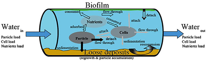
Figure 1 - Text description

An illustration showing the biological and physio-chemical interactions and reactions within the drinking water distribution system. The illustration shows a pipe section of the drinking water distribution system through which water is flowing from left to right. The water flowing into the pipe carries a load of particles, cells and nutrients. Once in the pipe, these particles, cells and nutrients are shown interacting with each other and with components of the pipe itself. Particles are shown falling to the floor of the pipe to join a layer of loose deposits (aka sedimentation). Other particles are shown detaching from the pipe wall (aka resuspension), while others are shown flowing through and exiting the pipe to join the participle load leaving the right side of the pipe. Nutrients are shown being consumed by the biofilm layer attached to the top of the pipe wall, and by cells and particles. Cells are shown attaching to particles and to the pipe floor, and exiting the pipe. Biofilm is shown detaching from the pipe wall.

B.1.1 Direct health risks

The degree to which water quality deterioration in the distribution system contributes to human illness is difficult to quantify because many events are not detected or recognized. In addition, rates of endemic infectious illness—including waterborne illness—are significantly underreported and underdiagnosed, for a number of reasons (Majowicz et al., 2004; MacDougall et al., 2008; Gibbons et al., 2014). This is further complicated by the fact that, in Canada, there is no national surveillance system specific to waterborne illness (Pons et al., 2015). Thus, there is very limited information regarding the magnitude and sources of waterborne illness in Canada, including those attributable to drinking water.

While Canadian surveillance data are scarce, United States (U.S.) surveillance data clearly show a link between distribution system contamination and human illness. Between 1995 and 2014, over 40 waterborne disease outbreaks attributed to distribution system deficiencies were reported in the U.S. (Levy et al., 1998; Barwick et al., 2000; Craun and Calderon, 2001; Lee et al., 2002; Blackburn et al. 2004; Liang et al. 2006; Yoder et al., 2008; Brunkard et al. 2011; CDC, 2013; Beer et al., 2015; Benedict et al., 2017). These resulted in over 4,800 cases of illness. A meta-analysis of U.S. data, conducted by the World Health Organization (WHO), showed that the majority of waterborne disease outbreaks attributed to distribution system were related to cross-connections (figure 2); and the most common etiological agent was bacteria (WHO, 2014). The release of biofilm and deposits in the distribution system, related to a water source change, was implicated in the Legionella outbreak that occurred in Flint, Michigan, U.S., between 2014 and 2015 (Rhoads et al., 2017; Zahran et al., 2018). Several international waterborne outbreaks attributable to the distribution system have also been reported (Nygård et al., 2004; Jakopanec et al., 2008; Moreira and Bondelind, 2017); including an extensive Finnish outbreak of gastroenteritis, affecting over 8,400 individuals, due to contamination of distributed water by sewage effluent (Laine et al., 2011).

Some epidemiological studies have reported an association between consumption of tap water from distribution systems and a negative impact on health (Hunter et al. 2005; NRC, 2006; Nygård et al., 2007; Córdoba et al., 2010; Lambertini et al., 2012; Ercumen et al., 2014; Säve-Söderbergh et al., 2017). Models used to explore public health impacts estimate that between 15 and 50% of waterborne gastrointestinal illness can be attributed to distribution system risks (Payment et al., 1997; Messner et al., 2006; Nygård et al., 2004, 2007; Murphy et al., 2016).

Figure 2 - Text description

An illustration showing two pie charts, A and B. Pie chart A illustrates the portion of distribution system-related outbreaks associated with a specific system fault. Cross-connections are the largest piece of the pie (42%), followed by: unknown causes (19%), water main breaks and repairs (each accounting for 11%), leaching (9%), storage (7%) and pressure fluctuation (1%). Pie chart B illustrates the portion of distribution system-related outbreaks associated with an etiological agent. Bacteria account for the largest piece of the pie (33%), followed by: protozoa (25%), chemical and unknown agents (each accounting for 14%), viruses (9%) and mixed microorganisms (5%).

B.1.2 Indirect health risks

The material accumulated within distribution systems (figure 1) becomes colonized with coliforms, heterotrophs, nitrifiers, iron-oxidizing bacteria and sulphur-reducing bacteria (Hill et al., 2018). Metal precipitates, including aluminum, iron, or manganese, within the deposits can act as an accumulation sink for other contaminants (e.g., arsenic, chromium, copper, lead) (Cantor 2017). These deposits can be disturbed and "released" in an uncontrolled manner due to hydraulic disturbances (e.g., fire-fighting activities, watermain breaks, pump station operation) or improper flushing operations. table 3 summarizes the concentrations of biological matter (also referred to as biomass) and metal precipitates measured in deposits removed from two full-scale systems using a range of flushing velocities. These data demonstrate that significant biomass and metal precipitates can accumulate and lead to deterioration in water quality. This may result in human illness if elevated concentrations of microorganisms or metals are consumed.

The release of microorganisms or metals is also generally associated with discolouration or turbidity events (Prince et al., 2003; Seth et al., 2004; Husband et al., 2016). Husband and Boxall (2010) reported that cast iron watermains consistently demonstrated higher turbidity with the release of accumulated material. Burlingame et al. (2006) reported a direct relationship between turbidity and the release of accumulated material from tuberculated iron pipes. Thus, consumer complaints of colour, or unpleasant taste and odour, can serve as an indicator of water quality deterioration in the distribution system (Hrudey and Hrudey, 2014). Coloured water should not be considered safe to consume until it has been tested and confirmed to be safe (Friedman et al., 2016).

Table 3. Biological matter and metal precipitate concentrations at various flushing velocities (Hill et al., 2018).

Community and pipe material	Velocity (ft/sec)	HPC-R2AFootnote a (cfu/mL)	Total viable biomassFootnote b (pg/mL)	Viable bacteriaFootnote c (cells/mL)	Iron (µg/L)	Manganese (µg/L)
A - cement-lined	4	930	9.3	89,200	4,000	800
	6	750	2.7	28,700Footnote d	4,400	180
	6	3,300	5.9	54,500Footnote d	6,400	200
A - cement-lined with unlined	6	380	4.0	34,000	4,300	330
A - unlined cast iron	3.0	130	1.2	20,700	3,700	140
	4.8	2,400	19	28,100	26,400	870
	6.0	430	2.0	37,900	15,100	300
	6.0	2,900	54	61,400	16,500	800
	6.4	1,030	4.7	31,300	7,500	210
B - unlined cast iron	3.0	1,470	270	590,700	193,100	20,600
	4.2	15,500	807	689,100Footnote d	139,000	30,100
	5.4	3,300	430	577,300	155,700	18,400
	6.0	1,500	280	601,500	199,000	20,900
	6.0	10,400	325	788,300Footnote d	153,300	11,300
Footnote a Heterothropic plate count (HPC) using R2A medium. Return to footnote a referrer Footnote b Measured using cellular adenosine triphosphate (cATP). Return to footnote b referrer Footnote c Measured using flow cytometry (FCM). Return to footnote c referrer Footnote d Includes total coliform-positive sample(s). Return to footnote d referrer

B.1.3 Distribution systems events or deficiencies

Between 2013 and 2019, watermain breaks and pressure losses in the distribution system were identified as the main reasons for issuing a boil water advisory in Canada, accounting for 72% of advisories (figure 3). These data are based on analyses of 5,578 records of boil water advisories, issued from 7 of 14 jurisdictions (Health Canada, 2019). A large waterborne outbreak of campylobacteriosis in Norway was attributed to pressure loss and poor distribution system integrity (Jakopanec et al., 2008). The lack of watermain disinfection following repair was also a contributing factor.

Fox et al. (2016) demonstrated that contaminants external to a small leak (5 mm diameter) in a pressurized pipe could enter the pipe and be transported within the system when negative transient pressures occur. Low and negative transient pressures can occur as a result of distribution system operation/maintenance or unplanned events such as power outages or watermain breaks. Low and negative transient pressures also allow contamination to enter the distribution system from cross connections and/or backflow from domestic, industrial or institutional facilities (Gullick et al., 2004).

Figure 3 - Text description

Figure 3 is a bar chart showing that the main reasons for issuing boil water advisories on public systems were; Line break or pressure loss in distribution system (72%), No applicable water quality reason (16%), Unacceptable turbidity or particle counts in treated water (4%), Total coliforms detected in drinking water system (3.4%), E. coli detected in drinking water system (2.7%), Significant deterioration of source water quality (0.8%), Suspected contamination (0.6%), Insufficient quantity (0.3%), Cross-connection with backflow suspected or confirmed (0.2%)

B.2 Causes of water quality deterioration

Ideally, there should be minimal change in water quality during distribution until the point of consumption. This concept is referred to as the biological stability of drinking water (van der Kooij, 2000; NRC, 2006; Lautenschlager et al., 2013; Prest et al., 2016b). Given the complexity and dynamic nature of distribution systems, significant changes in biological stability can occur, leading to deterioration in drinking water quality. Water quality deterioration in the distribution system is due to a multitude of factors and mechanisms (Figures 4 and 5). A brief discussion of select factors and mechanisms leading to deterioration in microbial water quality is provided below. For a more comprehensive review, please refer to LeChevallier, 1999; van der Kooij and van der Wielen, 2014; WHO, 2014; LeChevallier et al., 2015a,b; Prest et al., 2016a,b,c.

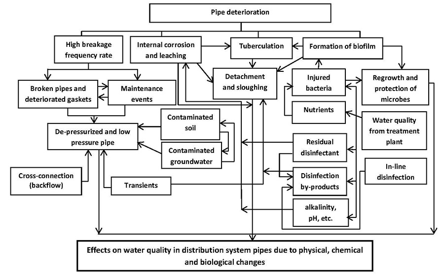
Figure 4 - Text description

A flowchart illustrating the complexity of factors and interactions within the drinking water distribution system that lead to deterioration of water quality. Multiple text boxes are shown, representing a wide range of factors, and their interactions, as highlighted by arrows. A range of factor types are illustrated, including those related to: pipe condition, intrusion events, general system conditions (e.g., pH, alkalinity), and presence of microorganisms, residual disinfectant and nutrients. As an example, pipe deterioration is linked with high breakage frequency rate, internal corrosion and leaching, tuberculation and formation of biofilm. Formation of biofilm, in turn, is linked with regrowth and protection of microorganisms, detachment and sloughing, and injured bacteria. These individual factors are then shown to be linked to variety of other factors, and so on and so forth.

B.2.1 Presence of microorganisms

Microorganisms can be present for two main reasons: 1) they are introduced into the distribution system or 2) conditions in the distribution system favour the (re)growth of microorganisms already present. Microorganisms can enter the distribution system by surviving the water treatment process or by intrusion. Intrusion occurs when there is an integrity breach, such as a pipe break or leak, and may result from short term pressure transients (LeChevallier et al., 2011). Several studies have demonstrated the potential for microbial contaminants to enter the distribution system (Karim et al., 2003; LeChevallier et al., 2003; Besner et al, 2010, 2011; Yang et al., 2011; Ebacher et al., 2012; Fontanazza et al., 2015; Fox et al., 2016). Multiple factors and mechanisms can promote microbial (re)growth, and are discussed in subsequent sections (Besner et al., 2012; Lee, 2013; LeChevallier et al., 2015a; Prest et al., 2016a,b,c; AWWA, 2017).

Drinking water distribution systems contain both attached (i.e., biofilm) and transient (i.e., planktonic) populations of microorganisms which can contribute to deteriorating water quality (figure 5). The combined genetic material of these microbial populations is known as the microbiome. The microbiome is impacted by numerous factors, including nutrient availability, pipe material, predation, and disinfectants (Zhang et al., 2017). Microbiomes are very heterogeneous, as well as time and site-specific both within and between distribution systems (Gomez-Alvarez et al., 2012; Chao et al., 2013, 2015; Delafont et al., 2013; Wang et al., 2014a,b; Zhang et al., 2017).

Biofilms are accumulations of microorganisms, typically encased in a matrix of extracellular polymeric substances (EPS), and containing both organic and inorganic matter, attached to the inner surfaces of pipes in drinking water distribution systems (Prest et al., 2016a; Liu et al., 2016; WRF, 2017). The EPS structure provides protection against predators and disinfectants, and aids in uptake and utilization of nutrients (LeChevallier et al., 1988; Flemming and Wingender, 2010; Prest et al., 2016a). Biofilms are ubiquitous in all distribution systems, and provide a habitat for the survival and growth of microorganisms, including pathogens (Health Canada, 2013b). A variety of enteric pathogens have been detected in biofilms (Park et al., 2001; Howe et al., 2002; LeChevallier et al., 2003; Chang and Jung, 2004; Berry et al., 2006; September et al., 2007; Gomez-Alvarez et al., 2015; Revetta et al., 2016); where they can accumulate and be released over an extended period of time (Howe et al., 2002; Warnecke, 2006; Wingender and Flemming, 2011). Non-enteric pathogens have also been detected in biofilms, including opportunistic premise plumbing pathogens (OPPPs), such as Legionella pneumophila and non-tuberculous mycobacteria (e.g., M. avium, M. intracellulare) (Falkinham et al., 2015; Wang et al., 2017). These organisms have adapted to grow and persist in distribution and plumbing system biofilms and have been linked to several outbreaks (Pruden et al.,2013; Beer et al., 2015; Falkinham et al., 2015; Benedict et al., 2017), including the 2014-15 Legionnaires' outbreak in Flint, Michigan, U.S. (Zahran et al., 2018). They represent a significant challenge to the water industry and building managers (see section B.4 Monitoring program).

Figure 5 - Text description

An illustration showing the microbial dynamics in a drinking water distribution system pipe. The illustration shows treated water entering a pipe section of the drinking water distribution system, and exiting at the tap. Treated water flowing into the pipe carries bacteria, particles, disinfectant residual and nutrients; and interacts with components of the pipe. Bacteria are shown consuming nutrients, attaching and detaching to/from the biofilm on the pipe wall, competing with other microbial cells, attaching to particles, and/or dying. Particles are shown falling to the floor of the pipe to join a layer of sediment, EPS and bacterial growth. Other particles are shown detaching from the pipe wall, binding to nutrients, and becoming resuspended. Nutrients are shown being consumed by the biofilm-EPS-sediment layer attached to the pipe wall and being released from the pipe wall (aka substrate leaching). Disinfectant residual is shown interacting with bacteria, leading to death and/or a microbial community shift; and interacting with the material attached to the pipe wall, along with suspended particles.

Bacterial indicator (i.e., total coliforms, E. coli) monitoring in the distribution system generally provides very little information about the microbiome because these indicators are seldom detected (Hargesheimer, 2001; U.S. EPA, 2016a). Also, the bulk water that is sampled only accounts for 2% of the total bacterial inventory; the material accumulated on the pipe wall accounts for the remaining (Liu et al., 2014). As a result, the water industry has historically used heterotrophic plate count (HPC) as an indicator of overall distribution system water quality (Hargeheimer, 2001). Even though HPC is a non-specific indicator and not associated with fecal contamination, they can be correlated to changes in distribution system water quality. For example, a decrease in disinfectant residual is generally associated with an increase in HPC. However, the requirement to not exceed an 8 hour holding time and the time to obtain results (2-7 days) can limit the use and benefits of HPC. An adenosine triphosphate (ATP) assay was developed to provide rapid measurements of total bacterial biomass (Lee and Deininger, 1999). Commercially available kits can produce results within minutes of sample collection (Whalen et al., 2006; Cantor, 2017; Hill et al., 2018). ATP measurements, along with disinfectant residual trends (e.g., are they decreasing), can very quickly provide an indication of increased microbial activity that requires follow-up actions. Additional information on HPC and ATP is provided in section B.3 Monitoring methods and parameters.

Monitoring for total coliforms and E. coli remains important as they are indicators of microbial integrity, potential unsanitary conditions or physical integrity issues and they form the basis for most regulatory compliance monitoring in Canada.

B.2.2 Type and availability of nutrients

A number of nutrients may be present in drinking water distribution systems, and can promote microbial growth, either by serving as fuel for microorganisms or by consuming disinfectant residual (NRC, 2006). The biodegradable portion of natural organic matter (NOM), referred to as biodegradable organic matter (BOM), for example, impacts distribution system water quality by providing a source of nutrients that contributes to microbial regrowth and biofilm development (Huck, 1990). Concentrations of BOM [e.g., Assimilable organic carbon (AOC) and biodegradable organic carbon (BDOC)] are only one component influencing changes in water quality in the distribution system (Prest et al., 2016a,b,c). Other nutrients have been identified as having roles in controlling microbial growth in the distribution system, including phosphorus, nitrogen, ammonia, manganese, sulphate, iron and humic substances (Camper, 2004, 2014; Coetser et al., 2005; Prest et al., 2016a,b,c). In some European countries, the approach taken to achieve biological stability is to minimize the concentrations of growth-supporting nutrients in water (Lautenschlager et al., 2013).

Water utilities should aim to minimize nutrients in treated water (e.g., organic carbon, ammonia, nitrate/nitrite, total phosphorus) and have a good understanding of their concentrations in the distribution system. This is particularly important for water utilities adding nutrients to their distribution system for chloramination (ammonia) or corrosion control (phosphorus).

B.2.3 Pipe material and condition

Pipes make up the majority of drinking water distribution systems, and their properties and condition can significantly impact drinking water quality. Pipe material can affect microbial regrowth, biofilm formation and composition. Typically, iron pipes favour microbial adhesion and growth (table 3) (Norton and LeChevallier, 2000; Niquette et al., 2000; Hill et al., 2018). Iron-oxidizing bacteria form raised outgrowths, called tubercles; these tubercles can harbour microorganisms, including opportunistic pathogens (Emde et al., 1992; U.S. EPA, 2002; Batté et al., 2003; NRC, 2006; Teng et al., 2008). As a result, the pipe wall can generate a significant disinfectant demand, making it difficult to maintain disinfectant residual concentrations. The tubercles can also generate colour, turbidity, tastes and odours, as well as reduce hydraulic efficiency (Husband and Boxall, 2010).

Other pipe materials (e.g., polyethylene cross-linked, polybutylene, polyvinyl chloride) have also been shown to impact microbial concentrations, diversity, resistance to disinfection (Zacheus et al., 2000; Donlan, 2002; Camper et al., 2003; Wingender and Flemming, 2004, 2011; van Der Kooij et al., 2005; Hyun-Jung et al., 2011; Yu et al., 2010; Wang et al., 2014a,b; Inkinen et al., 2018) and biofilm formation potential (van der Kooij and Veenendaal, 2001; Tsvetanova and Hoeskstra, 2008; Wen et al., 2015).

In addition to pipe material, pipe condition can significantly impact the microbial quality of drinking water in the distribution system (see figure 3). As pipes age, they become prone to leaks and breaks, corrosion and development of biofilm (O'Connor, 2002). Aging water infrastructure is a significant threat to water safety in Canada (Canadian Infrastructure Report Card, 2016). In Ontario, for example, many water systems were constructed in the 1960s and 1970s, (MacDonald, 2001) and, as such, will be nearing the end of their life span, which averages around 50 to 70 years (Tafuri and Field, 2010). Pipes installed during the 1960s and 1970s have also been associated with an increased likelihood of failure because of the type of material used, and poor installation practices (Besner et al., 2001; MacDonald, 2001). In other parts of Canada, pipes date back to before 1867 (Besner et al., 2001; Saint John Water, 2018).

B.2.4 Type and concentration of residual disinfectant

Residual disinfectant type and concentration also affect distribution system microbial water quality. In Canada, the majority of water utilities use free chlorine as a residual disinfectant; while the rest use chloramines (Health Canada, 2009). These disinfectants possess different capabilities in terms of disinfectant power, reactivity with organic and inorganic material and biofilm penetration. Free chlorine is highly effective at inactivating bacteria, but far less effective against protozoans; this may result in a significant change in bacterial community composition in the distribution system (Servais et al., 1995; Norton and LeChevallier, 2000; Roeder et al., 2010; Chiao et al., 2014; Nescerecka et al.,2014). The use of chloramines can lead to nitrification, the microbiological process whereby ammonia is sequentially oxidized to nitrite and nitrate by ammonia-oxidizing bacteria and nitrite-oxidizing bacteria, respectively (Wilczak, 2006). This can result in growth of nitrifying bacteria, leading to a loss in disinfectant residual and increased biofilm production, which further escalates the chlorine demand, ammonia release and microbial regrowth (Wilczak et al., 1996; Pintar and Slawson, 2003; Scott et al. 2015; Wilczak, 2006).

Minimum disinfectant residuals are typically recommended to control biofilm growth (LeChevallier et al., 1996; LeChevallier and Au, 2004); thus, decreases in disinfectant residual concentration can serve as a sentinel for water quality changes, such as increased microbial activity or physical integrity issues (LeChevallier, 1998; LeChevallier et al., 1996, 1998; Haas, 1999; NRC, 2006; Health Canada, 2020a,b; Nescerecka et al.,2014; Prest et al., 2016a). Variability in disinfectant residual concentrations—measured as the coefficient of variation— can be a useful indicator of biological stability (LeChevallier et al., 2015b), and is discussed in section B.3.1.1 Disinfectant residual concentrations and turbidity.

B.2.5 General distribution system conditions

Distribution system water quality can diminish considerably because of general system conditions, including hydraulic conditions, residence time, water temperature and pH. The following is a brief discussion of how these parameters can lead to deterioration of distribution system microbial water quality. For a more detailed discussion, refer to Health Canada, 1995, 2015; NRC, 2006; Nescerecka et al., 2014; LeChevallier et al., 2015a; Prest et al., 2016a; Zlatanovic et al., 2017.

Hydraulic changes in the distribution system are common and are highly dependent on water demand; in turn, water demand determines water age, which impacts water quality. During low demand periods, flow velocities decrease, leading to increased residence time. These conditions can result in water stagnation in parts of the distribution system, deposition of particles, and lead to circumstances favouring microbial (re)growth (Gauthier et al., 1999; Zacheus et al., 2001; Liu et al., 2013a, b). When there is high demand (i.e., hydraulic peaks), increases in flow rate can cause biofilm detachment and re-suspension of sediment (see figure 1) (Lehtola et al., 2006; Vreeburg and Boxall, 2007) leading to increased dispersal of microorganisms, including pathogens (Torvinen et al., 2004; Wingender and Flemming, 2011), release of metals (Friedman et al., 2010, 2016; Cantor, 2017; Hill et al., 2018) and colour or turbidity (Prince et al., 2003; Seth et al., 2004; Husband et al., 2016).

Water temperature and pH are important in various physical, chemical and biological processes occurring in the drinking water distribution system, and can impact water quality. Elevated water temperature, for example, can accelerate chlorine decay, leading to microbial growth (Li et al. 2003; van der Wielen and van der Kooij2010). Changes in pH and temperature also affects the solubility of metals (e.g., copper) present in distribution systems, with higher temperatures resulting in increased leaching and corrosion (Singh and Mavinic 1991; Boulay and Edwards 2001; Sarver and Edwards 2011); metals (e.g., aluminum) can also go in and out of solution depending on pH and temperature and be transported and deposited throughout the system (Driscoll et al., 1987; Halton, 2001; Snoeyink et al., 2003; Munk and Faure, 2004). In addition, higher water temperatures can promote biological processes, including microbial regrowth (LeChevallier et al., 1996; van der Kooij et al., 2003). Temperature fluctuations can impact biofilm attachment because of changing EPS production (Liu et al., 2016). As a result, changes in water temperature can significantly impact distribution system water quality. Although it is difficult to control temperature, water utilities should be aware of such changes and manage the impacts. With respect to pH, variability should be minimized to ±0.2 units to maintain chemical and biological stability (Muylwyk and MacDonald, 2001; Friedman et al., 2010; Health Canada, 2015). Information on the use of water temperature and pH as indicators of biological stability is provided in section B.3.1.3 Physical and chemical parameters.

B.3 Monitoring methods and parameters

Drinking water distribution systems are complex and dynamic environments. In order to understand changes in biological stability, a monitoring program (see section B.4 Monitoring program) should be designed and implemented to establish baseline conditions, monitor changes and detect on-going or potential contamination events. Comprehensive monitoring programs are recommended (Cantor, 2017, 2018; Hill et al., 2018) to obtain a better understanding of the microbial dynamics in the drinking water distribution system, thereby increasing the likelihood of detecting periods of higher risk. Multi-parametric approaches to monitoring the microbial quality of the distribution system are supported in the literature (Escobar and Randall, 2001; Hammes and Egli, 2005; van der Kooij, 2000; Berney et al., 2008; Vital et al., 2010, 2012; Hammes et al., 2011; Lautenschlager et al., 2013; Douterelo et al., 2014a; van der Kooij and van der Wielen, 2014; LeChevallier et al., 2015a,b; van der Kooij et al., 2015; Van Nevel et al., 2017).

Combining multiple methods and parameters affords a better understanding of distribution system dynamics and the potential impact on biological stability; this increases the likelihood of detecting periods of higher risk to human health. Use of multiple methods/parameters also facilitates more rapid detection of changes in the biological stability, so that efforts can be implemented in order to minimize risks to consumers (see section B.5 Managing microbiological risks).

For the purposes of the following discussion, potential methods or parameter analyses have been categorized as either: 1) rapid, 2) laboratory or 3) advanced in nature. Advanced methods may require partnership between water utilities and universities.

B.3.1 Rapid methods

B.3.1.1 Disinfectant residual concentrations and turbidity

Decreases in disinfectant residual concentration or increases in turbidity in the drinking water distribution system may be indicative of diminished biological stability (Cantor, 2017). Measuring the disinfectant residual and turbidity in the drinking water distribution system is important and should be done when bacterial indicator samples (see B.3.2.1 Bacterial indicators) are collected. Once data is collected, it should be analyzed to determine its variability. Variability, as measured by the coefficient of variation, can be a useful indicator of water quality stability (Cantor and Cantor, 2009; LeChevallier et al., 2015b). Another useful benchmark is to calculate the disinfectant demand/decay of the pipe wall deposits when conducting unidirectional flushing (Hill et al., 2018).

B.3.1.2 Adenosine triphosphate (ATP) analysis

Adenosine triphosphate measurements are gaining popularity as an indicator of total viable biomass in the distribution system (Ochromowicz and Hoekstra, 2005; Whalen et al., 2006; Siebel et al., 2008; Hammes et al., 2010; van der Wielen and van der Kooij, 2010; Nescerecka et al., 2016; Whalen et al., 2018); assays are low cost, easy to perform, and provide results in a matter of minutes. ATP is an energy molecule produced by all living organisms, and can be used as an indicator of microbial activity. A standard test method is available for detection of ATP content in microorganisms in water (ASTM International, 2015); and commercial kits, compliant with this method, are available.

The method consists of filtering water samples, followed by addition of a lysing agent in order to release cellular-ATP (cATP) from microbial cells captured on the filter (ASTM International, 2015). Luciferin-luciferase, a bioluminescence enzyme, is added, and the resulting light intensity is measured using a luminometer. The relative light units emitted are converted by comparison with an ATP standard, to provide the concentration of cATP in the sample (in pg ATP/mL) (ASTM International, 2015). This concentration is proportional to the number of viable microbial cells present in the sample. The method normally detects cATP concentrations ranging from 0.1 pg cATP/mL to 4 x 10⁶ pg cATP/mL in 50 mL water samples (ASTM International, 2015).

ATP measurements should be graphed and trends should be used and interpreted in conjunction with other monitoring results (Siebel et al., 2008; Hammes et al., 2010; Douterelo et al., 2014a; Nescerecka et al., 2014; Van Nevel et al., 2017). cATP concentrations above 1 pg/mL have been used to trigger actions to prevent increased microbial activity in chlorinated (Hill et al., 2018) and chloraminated (Ballantyne and Meteer, 2018) distribution systems.

Measuring the ATP accumulated on mild steel coupons placed in the distribution can be a useful measure of the biofilm formation rate (LeChevallier et al., 2015a,b).

B.3.1.3 Physical and chemical parameters

Water temperature, pH and oxidation-reduction potential are critical parameters that influence the life cycle of microorganisms and the solubility of metals in the distribution system. Data from these parameters can help explain trends and variations in distribution system water quality. For example, a high oxidation-reduction potential indicates a water quality that is not conducive to microbial growth (Cantor, 2018). These parameters should be analyzed in the field as changes can occur very quickly if water samples are in contact with air. Colour can also be associated with biofilm or metal releases (Husband and Boxall, 2010) and can be a useful indicator of water quality changes. It is recommended that apparent colour be measured (Hill et al., 2018).

B.3.2 Laboratory methods

B.3.2.1 Bacterial indicators

Routine monitoring of total coliforms and E. coli is a fundamental part of the source-to-tap approach to producing safe drinking water (CCME, 2004). The presence of these indicators in the distribution system, while absent immediately post-treatment, suggests that microbial contamination has occurred. The benefits and limitations of this approach have been discussed in section B.2.1 Presence of microorganisms, and in the Guidelines for Canadian Drinking Water Quality: Guideline Technical Documents for Escherichia coli and for Total Coliforms (Health Canada, 2020a,b).

B.3.2.2 Heterotrophic Plate Count (HPC)

Detection of heterotrophic microorganisms has traditionally been used to assess distribution system microbial water quality (Health Canada, 2012a). Heterotrophic microorganisms consist of bacteria, moulds, and yeasts that require organic carbon for growth (Leclerc, 2003). These organisms are naturally present in the environment, including water. They can be measured using HPCs (APHA et al., 2017). Standard HPC methods use colony formation on culture media to approximate the concentration of heterotrophs in a drinking water sample (Lillis and Bissonette, 2001; Reasoner, 2004; APHA et al., 2017). Although no single growth medium, temperature, or incubation time will ensure the recovery of all heterotrophs, including those that might be injured, use of R2A agar has proven most sensitive (Deininger and Lee, 2001; Uhl and Schaule, 2003; Gagnon et al., 2007; Rand et al., 2014, AWWA, 2017).

HPC data significantly underestimate the concentration and diversity of bacteria present in the drinking water distribution system (WHO, 2003; Van Nevel et al., 2017) and do not reflect the behaviour of the microbiome (Proctor and Hammes, 2015; Bautista-de los Santos et al., 2016). As such, HPC is not an indicator of microbial presence in the distribution system. Instead, HPC data, acquired using R2A agar, can provide meaningful information regarding water quality changes that may impact biological stability (Gagnon et al., 2007; Rand et al., 2014).

B.3.2.3 Nutrient concentrations

As nutrients (e.g., organic carbon, ammonia, nitrate/nitrite, total phosphorus) contribute to bacterial (re)growth and biofilm development, water utilities should aim to minimize their concentration in treated water and have a good understanding of their concentrations in the distribution system. It is recommended that total or dissolved organic carbon be monitored (LeChevallier et al., 2015a,b; Cantor, 2017; Hill et al., 2018). For water utilities that are using chloramination, it is important to monitor for nitrification events (e.g., total and free ammonia, nitrite, nitrate). For water utilities using phosphate-based corrosion inhibitors, monitoring throughout the distribution system is necessary to ensure a consistent disinfectant residual concentration, thereby, promoting the stability of inhibitors.

B.3.2.4 Metals

The complex and dynamic environment found within distribution systems results in metal precipitates being bound into the biofilm and deposits. This may be as a result of water quality characteristics or pipe material. Hydraulic disturbances can cause the release of elevated metals concentrations. Metals can be present in dissolved or particulate form. For distribution system monitoring, it is acceptable to consider the particulate form to be the difference between the total and dissolved metal concentration. In order to determine dissolved concentrations, samples should be filtered at the time of collection (not at the laboratory). At a minimum, monitoring should be conducted for the metals that are major accumulation sinks (e.g., aluminum, iron and manganese) for other health-based contaminants. In addition, it is recommended that key health-based contaminants that are known to accumulate be monitored (e.g., arsenic, lead and any other site-specific parameters for which treatment is in place). Some laboratories offer a long list of metals for one price per sample. In this case, the full scan of metals is recommended to obtain useful information regarding scale formation and dissolution (Cantor, 2017).

B.3.3 Advanced methods

B.3.3.1 Flow cytometry (FCM)

FCM is one of the leading methods for monitoring of microbial water quality in the distribution system (Prest et al., 2013, 2016a,b,c; Douterelo et al., 2014a; Van Nevel et al., 2017). This method characterises and quantifies suspended particles by passing them one at a time through a laser beam (Shapiro, 2003; figure 6). The laser beam excites fluorescent particles which then emit light at a higher wavelength. It is important to note that biological particles can be made fluorescent, as in the case of bacteria that have been stained with a fluorescent dye (e.g., SYBR Green I), or can naturally be fluorescent (e.g., chlorophyll-containing algae) (Hammes and Egli, 2010). Flow cytometry possesses a number of advantages and disadvantages (table 4).

Interpretation of flow cytometry results is complicated because of the wealth of data generated and the lack of standardized analysis methods (Hammes and Egli, 2010; Van Nevel et al., 2017). In general, changes in flow cytometric cell counts are indicative of a potential problem and should be investigated. In order to accurately identify these changes, it is essential to establish microbial concentrations under normal conditions (i.e., a baseline) (Besmer et al., 2014). This necessitates widespread and long-term monitoring of the drinking water distribution system to determine flow cytometric cell counts under various conditions, and during different seasons (Besmer et al., 2014, 2016). Thus, application of flow cytometry for routine monitoring of the drinking water distribution system requires at least a few years of gathering data, in concert with other microbial monitoring methods, in order to accurately interpret results (Van Nevel et al., 2017).

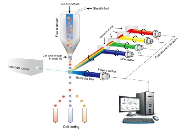
Figure 6 - Text description

An illustration showing the principles of flow cytometry. The illustration shows a (stained) cell suspension, represented by a liquid made up of a mixture of small red, yellow and blue spheres, entering a funnel-like apparatus, called a flow chamber. The spheres (cells) exit the chamber in single file - i.e., one at a time. As each sphere (cell) exits, it is shown passing through a beam of light from a laser, shown as a box labeled "light source". The sphere (cell) is shown becoming excited, as represented by a burst of light, and emitting fluorescence - a rainbow of red, yellow, green and blue. This process is magnified on the right side of the illustration, where colors are shown as separate beams of light that link back to a fluorescence detector, represented by a thin cylinder (for each color) with a grey top hat, and separated by mirrors. Like-colored spheres (cells) are shown entering the same test tube after their fluorescent is recorded, as represented by an image of a computer.

Table 4. Advantages and disadvantages of flow cytometry.

Advantages	References
Able to measure changes in bacterial cell counts	Lautenschlager et al., 2013; Prest et al., 2013, 2016a,b,c; Nescerecka et al., 2014
Rapid (~15 minutes), accurate and quantitative	Van Nevel et al., 2017
Highly reproducible (e.g., relative standard deviations less than 2.5 for a single operator and machine)	Hammes et al., 2008; Wang et al., 2010; Prest et al., 2013
Amenable to automation which allows for high throughput (i.e., multi-well plate analysis feature permits analysis of up to 500 samples within a day)	Van Nevel et al., 2013
Online technology allows continuous FCM measurements for several subsequent weeks	Hammes et al., 2012; Brognaux et al., 2013; Besmer et al., 2014; Prest et al., 2013, 2016a,b,c
Able to distinguish low nucleic acid cells from high nucleic acid cells	N/A
Standardized method available in Europe, facilitating comparison between laboratories	SLMB, 2012; Prest et al., 2013
Detailed characterization of bacterial communities using FCM fingerprints	De Roy et al., 2012; Prest et al., 2013; Koch et al., 2014
FCM fingerprints permit increased sensitivity in detecting small changes and shifts within the bacterial community, and consistent with 16 rRNA gene analysis	De Roy et al., 2012; Prest et al., 2013; Koch et al., 2014; Props et al., 2016
Considerable requirements for equipment, user training, and data processing	Hammes and Egli, 2010
Difficulties in distinguishing between viable and non-viable bacteria, thus, requirement for appropriate viability staining	Berney et al., 2008; Helmi et al., 2014
Comparison of FCM data generated by different instrument types	N/A
Subjective counting process (i.e., manual gating)	Hammes and Egli, 2010; De Roy et al., 2012; Aghaeepour et al., 2013; Prest et al., 2013
Does not discriminate between single cells or clumps (e.g., sloughed biofilm), potentially leading to undercounting	Shapiro, 2003; van der Kooij and van der Wielen, 2014
Limited number of studies in drinking water distribution systems using a disinfectant residual	Van Nevel et al., 2017
Standardized methods have not yet been developed for drinking water applications	Hammes and Egli, 2010; Lautenschlager et al., 2013; Prest et al., 2013

B.3.3.2 Molecular methods

A variety of molecular methods are available to assess microbial community diversity in drinking water distribution systems (Norton and LeChevallier 2000; Eichler et al. 2006; Henne et al. 2012; Pinto et al. 2012; Liu et al., 2013a,b; Prest et al., 2013, 2014, 2016a,b,c; Vierheilig et al., 2015; Ling et al., 2016; Van Nevel et al., 2017). These methods generally rely on comparison of nucleic acid [Deoxyribonucleic acid (DNA) or Ribonucleic acid (RNA)] fingerprints and/or sequences to discern the composition of microbial communities. Typically, water or biofilm samples are processed in order to isolate DNA and/or RNA, and this nucleic material is then amplified using the polymerase chain reaction (PCR); PCR targets specific marker genes, including16S rRNA for bacteria, 18S rRNA for eukaryotes, and ITS for fungi. Amplification products are electrophoresed, and then bands (on the gel) are excised and sequenced; sequences are analyzed phylogenetically. A variety of next generation sequencing technologies are available which have a number of advantages over traditional methods, including real-time targeted sequencing and portability (Tan et al., 2015; Goordial et al., 2017; Liu et al., 2018).

Molecular approaches have several advantages. However, they also suffer from some significant shortcomings (table 5) which have limited their application for routine monitoring of drinking water distribution systems.

Table 5. Advantages and disadvantages of molecular approaches.

Advantages	References
Cultivation-independent	N/A
Allow for additional (future) analyses by freezing extracted nucleic acid	Van Nevel et al., 2017
Ability to identify viable microorganisms when RNA is extracted	Van Nevel et al., 2017
NGS technologies permit real-time sequencing	Tan et al., 2015; Goordial et al., 2017
Can be used for source tracking (i.e., determining origin of contamination)	Liu et al., 2018
Inadequate detection limit (i.e., dependent on target gene and sequence length) and difficulties with viability assessment	Nocker et al., 2007, 2017
Time-intensive nucleic acid extraction	Nocker et al., 2007, 2017; Hwang et al., 2011, 2012; Salter et al., 2014
PCR amplification bias (i.e., choice of target and primers)	Nocker et al., 2007, 2017; Hwang et al., 2011, 2012; Salter et al., 2014
Varying assumptions and approaches to extraction, and fingerprint/sequence analysis and interpretation	N/A
Limited representativeness of microbial diversity (i.e., bias towards most abundant microbial community members)	Hug et al., 2016
Costly and requires specialised molecular biology training	N/A

B.3.3.3 Biofilm analysis

The majority of microorganisms in drinking water distribution systems are attached to internal pipe surfaces, forming biofilms (Flemming et al., 2002). Biofilm analysis is a key component of understanding changes in microbial quality in the distribution system. As distribution system pipes are not readily accessible, collection of biofilm samples is very challenging; and biofilm analysis involves specialized methods that may require partnership between water utilities and universities or advanced commercial laboratories.

Typically, bench-top laboratory biofilm reactors are used to study biofilm formation under simulated conditions. Although these reactors significantly aid our understanding of potential changes in biofilm, they cannot fully replicate the conditions of real drinking water distribution systems (Deines et al., 2010). As such, more recent methods have focussed on analysis of biofilms in situ (i.e., in the actual distribution system). The most widely used approaches involve studying biofilms formed on cut-outs of distribution pipes (LeChevallier et al., 1998; Wingender and Flemming, 2004, 2011) or coupons inserted into pipes (Douterelo et al., 2013, 2016a,b). Biofilms can also be studied by flushing the pipes and collecting the material that has been mobilized into the bulk water (Douterelo et al., 2014b), or by sampling biofilm from household water meters (Hong et al., 2010; Ling et al., 2016). Although these approaches have their limitations, coupon-based methods show promise because they permit visualization of biofilm using microscopic methods, and nucleic acids can be extracted for characterization (Douterelo et al., 2014a).

B.3.3.4 Sensors and modeling

Online sensors have traditionally been used to monitor physical (e.g., pressure) and chemical (e.g., chlorine residual) parameters in the drinking water distribution system. Biologicalsensors (biosensors) are also available for real-time detection of microorganisms in the distribution system (U.S. EPA, 2009; Miles et al., 2011; Storey et al., 2011; Samendra et al., 2014; Højris et al., 2016; U.S. EPA, 2018a). Multi-parameter in-line sensors are also available to conduct real-time monitoring of important distribution system parameters, including chlorine, conductivity, pressure and temperature (Durand et al., 2016). In addition, approaches for monitoring the microbial quality of distribution systems, such as ATP and flow cytometry, have been automated for on-line detection.

Water distribution system models can aid in understanding changes in microbial water quality, and in developing monitoring and sampling approaches. These computer models take into consideration the hydraulics of the distribution system, along with other characteristics (Powell et al., 2004; Martel et al. 2006; Speight and Khanal, 2009), in order to simulate the fate of microbial contaminants. A number of models are available, including the U.S. Environmental Protection Agency (U.S. EPA)'s open-source drinking water distribution system model, referred to as EPANET (U.S. EPA, 2018b). An EPANET module, referred to as EPANET-MSX (Multi-Species Extension), considers interactions between the bulk water and pipe walls.

Quantitative microbial risk assessment (QMRA) models can also be used in conjunction with hydraulic models to better understand deteriorating microbial water quality in distribution systems (Blokker et al., 2014, 2018).

B.4 Monitoring program

B.4.1 Comprehensive monitoring program

Table 2 (see Part A) outlines the potential parameters and methods that can form the basis of a comprehensive monitoring program to assess the biological stability of drinking water in the distribution system. Many of the listed parameters (e.g., disinfectant residual, turbidity) are already being monitored as part of a source-to-tap approach to producing safe drinking water. Other parameters/methods are relatively easy to use and provide rapid results (see section B.3.1.2 Adenosine triphosphate (ATP) analysis and section B.3.1.3 Physical and chemical parameters).

The key is to use the most appropriate measures to routinely monitor distribution water quality and establish baseline conditions (e.g., normal variations not requiring action). It is important to recognize that distribution systems differ significantly in their design, size and complexity, therefore, no single monitoring program will meet the needs of all systems. Instead, water utilities should develop a monitoring program based on a system-specific assessment, and consider the cost and ease-of-use of monitoring methods, as well as the requirements of the responsible drinking water authority.

System-specific water quality goals and targets that trigger preventive or correction actions can then be established (Cantor and Cantor, 2009; Ballantyne and Meteer, 2018). Once data is collected, it should be analyzed to assess if, and how, distribution system water quality is changing and if preventive or corrective actions are necessary (see section B.4.4 Data analyses and response).

B.4.2 Sampling frequency

The sampling frequency ultimately depends on a system-specific assessment of the distribution system, including its size and complexity, in combination with any requirements established by the responsible drinking water authority. For example, sampling frequency should be increased in accordance with the size of the population served. Guidance on sampling for microbial indicators (i.e., E. coli and total coliforms) in the distribution system is available in Canada (Health Canada, 2020a,b) and globally (U.S. EPA, 2013; WHO, 2011, 2014). Water utilities should assess which parameters can be measured in the field or sampled when collecting microbial indicator samples. Practical guidance on monitoring and evaluating distribution system water quality is available in Cantor (2018).

B.4.3 Sampling locations

Careful consideration should be given to identifying locations within the drinking water distribution system where the risk of microbial contamination is likely highest. This requires an understanding of the distribution system through a detailed description of the location of major transmission components and distribution mains. Distribution system layout details, such as the location of storage facilities, pumps, valves, meters and consumer connections, need to be considered. Additional system attributes, including pipe material and age, are important to capture when determining where to sample. Historical water quality data are also integral to informing selection of monitoring locations. These data can highlight locations where risk of microbial deterioration is highest. It is also important to consider water demand (i.e., hydraulic changes) and where previous contamination has occurred. Watermain age and breakage records, for example, can be reviewed to identify possible higher risk locations. Prior detections of microbial indicators (e.g., total coliforms, E. coli, HPC) are also an important factor to consider when choosing where to monitor. The types of buildings (e.g., schools, hospitals) supplied by the distribution system should also be considered, as they represent a higher number of potential exposures.

The composition of the sampling tap must be considered when determining sampling locations, as it can affect microbial test results (Geldreich et al, 1985; Cox and Giron, 1993; Goatcher et al, 1992; Geldreich and LeChevallier, 1999). Water distribution system models can integrate distribution system features and water quality data in order to develop monitoring and sampling approaches (refer to section B.3.3.4 Sensors and modeling).

In addition to distribution system characteristics and water quality data, selection of monitoring locations will depend on the requirements of the responsible drinking water authority. In Quebec (Canada), for example, at least half of samples must be collected at the outermost boundary of the distribution network (Islam et al., 2015). Thus, the responsible drinking water authority should be consulted when identifying sampling locations.

In general, the entry point to the distribution system and points near dead-end zones and poor hydraulics (i.e., high water age) should be targeted for monitoring (Islam et al., 2015; Cantor, 2017). Once possible sampling locations have been identified, it is important to ensure that they are spatially representative (Vital et al., 2012; Nescerecka et al., 2014; Hill et al., 2018). In the U.S., for example, U.S. EPA's Revised Total Coliform Rule ensures spatial representativeness by allowing the collection of samples from dedicated distribution system sampling stations (U.S. EPA, 2013; LeChevallier, 2014). Consideration should also be given to rotating among sampling sites throughout the distribution system as this may improve detection (WHO, 2014).

B.4.4 Data analyses and response

Data generated using a routine distribution system monitoring program should be tracked to evaluate trends and variability. This will allow systems to determine baseline water quality conditions, and thus, identify if, and how, the biological stability is changing in the distribution system. Water utilities can then establish water quality goals for the distribution system. For example, a system may wish to establish a free chlorine residual of 0.4 mg/L rather than 0.2 mg/L, or it may wish to establish a threshold for HPCs or cATP as an early indicator of deterioration in microbial water quality. System-specific alert and action limits should also be established to trigger preventive or corrective actions (Cantor and Cantor, 2009). If water quality goals are not met, system-specific preventive or corrective actions should be taken (Ballantyne and Meteer, 2018).

More detailed information on water quality monitoring data management and analysis is available elsewhere (Cantor and Cantor, 2009; AWWA, 2017; Cantor 2018).

B.5 Managing microbiological risks

The drinking water distribution system is the last protective barrier before the consumers' tap. A well-maintained and operated distribution system is a critical component of providing safe drinking water. Although drinking water distribution systems can vary considerably, they face common challenges, including water quality deterioration (see section B.2 Causes of water quality deterioration). In order to ensure delivery of safe drinking water to consumers, the causes of this deterioration need to be understood. It is recommended that water utilities develop a distribution system monitoring plan to identify sources of contamination and/or causes of (re)growth. The results of this monitoring inform selection of appropriate risk management strategies (i.e., best practices). Some key best management practices for minimizing microbial risks in the distribution system are briefly detailed below. Comprehensive reviews of these practices can be found elsewhere (NRC, 2006; Kirmeyer et al., 2014; Mosse and Murray, 2015; Cantor, 2018).

In general, strategies to minimize microbial risks from the drinking water distribution system include:

• Treatment optimization to minimize nutrients entering into the system (e.g., organic carbon, ammonia, nitrite/nitrate, total phosphorus);
• Manage water age;
• Manage impacts of water temperature;
• Maintain an effective disinfectant residual;
• Maintain pH within ±0.2 units;
• Keep the distribution system clean;
• Maintain positive pressure; and
• Minimize physical and hydraulic disturbances.

Other measures that contribute to maintaining stable chemical and biological conditions in the distribution system include backflow prevention and cross-connection control; corrosion control; and maintenance and cleaning of distribution system pipes (Karim et al., 2003; Prévost et al., 2005; Fleming et al., 2006; Friedman et al., 2009; van der Kooij and van der Wielen, 2014; WHO, 2014; LeChevallier et al., 2015a,b; Friedman et al., 2016; Prest et al., 2016a,b,c). A variety of pipe cleaning strategies, aimed at removing biofilm, loose deposits and sediment, are available, including unidirectional flushing and pigging (Ellison, 2003; Bellas and Tassou, 2005, Quarini et al., 2010, Vreeburg et al., 2010; Dang et al., 2014; Friedman et al., 2016; Liu et al., 2017). In addition, strict hygiene should be practiced during all watermain construction, repair or maintenance to ensure drinking water is transported to the consumer with minimum loss of quality (Kirmeyer et al., 2001, 2014).

Caution is needed when using flushing. It is important that water utilities identify and implement the most appropriate flushing technique to avoid disturbing and releasing legacy deposit into the bulk water. Improper flushing techniques can stir up and potentially spread contaminants around the flushed area or deeper into the distribution system, thus increasing public health risk. The following conditions can disturb legacy deposits: excessive flushing rate or velocity; insufficient flushing rate or velocity; lack of directional control; and, inadequate flush duration (Hill et al., 2018). Automatic flushing stations are recommended if the goal is to turnover bulk water in an area due to water age or poor circulation (Hill et al., 2018).

Comprehensive reviews of biological stability can be found elsewhere (Prévost et al., 2005; van der Kooij and van der Wielen, 2014; LeChevallier et al., 2015a; Prest et al., 2016a,b,c). Guidance to help water utilities establish an appropriate system-specific monitoring program is also available (LeChevallier et al., 2015b; Cantor, 2017, 2018; Hill et al., 2018).

B.5.1 Microbial risk in buildings/premise plumbing

Premise plumbing refers to the portion of drinking water distribution system beyond the property line and in schools, hospitals, public and private housing, offices and other buildings (NRC, 2006; U.S. EPA, 2016). Water use in buildings includes drinking, food preparation, washing and showering, cooling systems and features (e.g., ornamental fountains).

Water quality can diminish significantly in building premise plumbing and is influenced by the same factors as those in drinking water distribution systems (see section B.2 Causes of water quality deterioration). However, building (premise) plumbing systems face some additional challenges, including: 1) longer residence times (i.e., increased water stagnation); 2) increased water temperatures; 3) use of a variety of plumbing components and materials; and 4) small pipe diameters. Long residence times in premise plumbing have been linked to significantly higher concentrations of microbial populations, and shifts in microbial community composition (Pepper et al., 2004; Lautenschlager et al., 2010; Manuel et al., 2010; Lipphaus et al., 2014; Bédard et al, 2018). Higher water temperatures, due to pipes being installed in heated rooms or near heat sources, promote microbial (re)growth (Lautenschlager et al., 2010; Lipphaus et al., 2014). (Re)growth is also enhanced through interaction with various plumbing materials, such as plastic tubing and rubber fittings, which have considerable microbial growth promotion potential (Bucheli-Witschel et al., 2012). Smaller pipe diameters result in increased contact between microorganisms and pipes, leading to enhanced pipe material impacts (see section B.2.3 Pipe material and condition), including biofilm formation and lowered disinfectant residual concentrations (Servais et al., 1992; Rossman et al., 1994; Prévost et al., 1998). As noted earlier (see section B.2.1 Presence of microorganisms), these biofilms can harbour pathogens, including OPPPs. Premise plumbing systems can dramatically enhance the growth of Legionella sp. and other OPPPs, such as Pseudomonas aeruginosa and non-tuberculous Mycobacteria, and are a significant public health concern, particularly, in hospitals (WHO, 2011)

Premise plumbing can also impact water quality in the distribution system. The main mechanism by which microbial contamination can enter the drinking water distribution system from building premise plumbing is through backflow, either by back-siphonage or back pressure (WHO, 2011, 2014). Thus, it is important that appropriate backflow and cross-connection control programs are in place (AWWA, 2017).

Given the unique water quality challenges present in buildings, additional management strategies are required. It is important to note that water utilities are not generally responsible for water quality from the property line to individual points of use in buildings. Building owners or managers must monitor and manage their water systems in order to ensure safe water at the consumers' tap. Management of water quality in buildings begins with accurate and up-to-date maps of building water systems and labeling of pipework, particularly in large buildings. These are important tools to help avoid dangerous cross-connections, and identify zones were water can stagnate.

Although it is beyond the scope of this document to specify where, when and how to routinely monitor premise plumbing, some guiding principles include:

• Environmental sampling for bacteria should not occur in isolation, but as a part of a comprehensive building water management program.
• Sampling plans are unique to each building and should be based on building characteristics (e.g., size, age, layout, population served) and historical water quality data (e.g., trend analysis of previous bacterial test results, water quality parameters such as disinfectant residual and temperature).
• Water quality can vary between floors, outlets and hot and cold water taps; sites that may produce water aerosols should be considered for sampling.
• A sampling approach can be adapted based on trends and system changes.
• If impacts from microbial growth are detected (e.g., discoloured water, unpleasant tastes or odours, and slimes in water-using devices), corrective actions such as flushing or disinfection may be needed in the building water system.

Detailed information on managing water safety in buildings is available elsewhere (WHO, 2011; Health Canada, 2013a; Public Works and Government Services Canada, 2013; ASHRAE, 2000, 2015, 2018).

Part C: References

• Aghaeepour, N., Finak, G., Hoos, H., Mosmann, T.R., Brinkman, R., Gottardo, R., Scheuermann, R.H., Dougall, D., Khodabakhshi, A.H., Mah, P., Obermoser, G., Spidlen, J., Taylor, I., Wuensch, S.A., Bramson, J., Eaves, C., Weng, A.P., Fortuno III, E.S., Ho, K., Kollmann, T.R., … Vilar, J.M.G. (2013). Critical assessment of automated flow cytometry data analysis techniques. Nat. Methods, 10(3): 228-238.
• APHA, AWWA, WEF (2017). Standard methods for the examination of water and wastewater. 23rd edition. Standard methods for the examination of water and wastewater. American Public Health Association, American Water Works Association and Water Environment Federation, Washington, DC.
• ASHRAE (2000). Guideline 12-2000: Minimizing risk of legionellosis associated with building water systems.
• ASHRAE (2015). Standard 188-2015: Legionellosis risk management for building water systems (ANSI approved).
• ASHRAE (2018). Standard 188-2018 : Legionellosis risk management for building water systems (ANSI approved).
• ASTM International. (2015). ASTM D4012 - 15: standard test method for adenosine triphosphate (ATP) content of microorganisms in water. In Annual book of ASTM standards. West Conshohocken, PA.AWWA (2017). Water quality in distribution systems. AWWA manual of water supply practices M68. American Water Works Association, Denver, CO.
• AWWA (2017). Water quality in distribution systems. AWWA manual of water supply practices M68. American Water Works Association, Denver, Colorado.
• Ballantyne, L. and Meteer, L. (2018). Nitrifying nightmares and how to avoid them. Ontario Water Works Association Annual Water Conference, Niagara Falls, ON.
• Barwick, R.S., Levy, D.A., Craun, G.F., Beach, M.J. and Calderon, R. (2000). Surveillance for Waterborne-Disease Outbreaks - United States 1997-1998. Morb. Mortal. Wkly. Rep., 49:4:1.7:5:1.
• Batté, M., Appenzeller, B.M.R., Grandjean, D., Fass, S., Gauthier, V., Jorand, F., Mathieu, L., Boualam, M., Saby, S. and Block, J.C. (2003). Biofilms in drinking water distribution systems. Rev. Environ. Sci. Biotechnol., 2(2-4): 147-168.
• Bautista-De los Santos, Q.M., Schroeder, J.L., Sevillano-Rivera, M., Sungthong, R., Ijaz, U.Z., Sloan, W.T. and Pinto, A.J. (2016). Emerging investigators series: Microbial communities in full-scale drinking water distribution systems-a meta-analysis. Environ Sci: Water Res and Technol., 2(4): 631-644.
• Bédard, E., Laferrière, C., Déziel, E. and Prévost, M. (2018). Impact of stagnation and sampling volume on water microbial quality monitoring in large buildings. Plos One, 13(6).
• Beer, K.D., Gargano, J.W., Roberts, V.A., Hill, V.R., Garrison, L.E., Kutty, P.K., Hilborn, E.D., Wade, T.J., Fullerton, K.E. and Yoder, J.S. (2015). Surveillance for waterborne disease outbreaks associated with drinking water - United States, 2011-2012. MMWR Morb. Mortal. Wkly. Rep., 64(31): 842-848.
• Bellas, I. and Tassou, S.A. (2005). Present and future applications of ice slurries. Int. J. Refrigeration 28, 115-121.
• Benedict, K.M., Reses, H., Vigar, M., Roth, D.M., Roberts, V.A., Mattioli, M., Cooley, L.A., Hilborn, E.D., Wade, T.J., Fullerton, K.E., Yoder, J.S. and Hill, V.R. (2017). Surveillance for waterborne disease outbreaks associated with drinking water - United States, 2013-2014. Morb. Mortal. Wkly. Rep., 66(44): 1216-1221.
• Berney, M., Vital, M., Hulshoff, I., Weilenmann, H.U., Egli, T. and Hammes, F. (2008). Rapid, cultivation-independent assessment of microbial viability in drinking water. Water Res., 42(14): 4010-4018.
• Berry, D., Xi, C. and Raskin, L. (2006). Microbial ecology of drinking water distribution systems. Curr. Opin. Biotechnol., 17(3): 297-302.
• Besmer, M.D., Weissbrodt, D.G., Kratochvil, B.E., Sigrist, J.A., Weyland, M.S. and Hammes, F. (2014). The feasibility of automated online flow cytometry for in-situ monitoring of microbial dynamics in aquatic ecosystems. Frontiers in Microbiology, 5.
• Besmer, M.D., Epting, J., Page, R.M., Sigrist, J.A., Huggenberger, P. and Hammes, F. (2016). Online flow cytometry reveals microbial dynamics influenced by concurrent natural and operational events in groundwater used for drinking water treatment. Sci. Rep., 6: 38462.
• Besner, M-C., Gauthier, V., Barbeau, B., Millette, R., Chapleau, R. and Prévost, M. (2001). Understanding distribution system water quality. J. Am. Water Works Assoc., 93 (7): 101-114.
• Besner, M-C., Ebacher, G., Jung, B.S., Karney, B., Lavoie, J., Payment, P. and Prévost, M. (2010). Negative pressures in full-scale distribution system: Field investigation, modelling, estimation of intrusion volumes and risk for public health. Drinking Water Engineering and Science, 3(2): 101-106.
• Besner, M-C., Prevost, M. and Regli, S. (2011). Assessing the public health risk of microbial intrusion events in distribution systems: Conceptual model, available data, and challenges. Water Res., 45(3): 961-979.
• Besner, M.C., Modak, P.R. and Glauser, N. (2012). Extensive sediment characterization during unidirectional flushing in a distribution system. 14th Water Distribution System Analysis Conference, v. 2, pp. 871-876.
• Blackburn, B.G., Craun, G.F., Yoder, J.S., Hill, V., Calderon, R.L., Chen, N., Lee, S.H., Levy, D.A. and Beach, M.J. (2004). Surveillance for waterborne-disease outbreaks associated with drinking water - United States, 2001-2002. MMWR Surveill. Summ., 53(8): 23-45.
• Blokker, M., Smeets, P. and Medema, G. (2014). QMRA in the drinking water distribution system. Procedia Eng., 89: 151-159.
• Blokker, M., Smeets, P. and Medema, G. (2018). Quantitative microbial risk assessment of repairs of the drinking water distribution system. Microb. Risk Anal., 8: 22-31.
• Boulay, N. and Edwards, M. (2001). Role of temperature, chlorine, and organic matter in copper corrosion byproduct release in soft water. Water Res., 35(3): 683-690.
• Brognaux, A., Han, S., Sørensen, S.J., Lebeau, F., Thonart, P. and Delvigne, F. (2013). A low-cost, multiplexable, automated flow cytometry procedure for the characterization of microbial stress dynamics in bioreactors. Microb. Cell Fact.,12(1).
• Brunkard, J.M., Ailes, E., Roberts, V.A., Hill, V., Hilborn, E., Craun, G.F. and Rajasingham, A. (2011). Surveillance for Waterborne Disease Outbreaks Associated With Drinking Water - United States, 2007-2008. Morb. Mortal. Wkly. Rep., Surveill Summ, 60:12:38.
• Bucheli-Witschel, M., Kötzsch, S., Darr, S., Widler, R. and Egli, T. (2012). A new method to assess the influence of migration from polymeric materials on the biostability of drinking water. Water Res., 46(13): 4246-4260.
• Burlingame, G.A. Lytle, D.A. and Snoeyink, V.L. (2006). Why red water? Understanding iron release in distribution systems. Opflow, 32 (12): 12-16.
• Camper, A.K. (2004). Involvement of humic substances in regrowth. Int. J. Food Microbiol., 92(3): 355-364.
• Camper, A. (2014). Organic matter, pipe materials, disinfectants and biofilms in distribution systems. In: Microbial growth in drinking-water supplies: Problems, causes, control and research needs. van der Kooij, D. and van der Wielen, P.W.J.J. (eds.). IWA Publishing, London, UK, pp. 73-94.
• Camper, A.K., Brastrup, K., Sandvig, A., Clement, J., Spencer, C. and Capuzzi, A.J. (2003). Effect of distribution system materials on bacterial regrowth. J. Am. Water Works Assoc., 95(7): 107-121.
• Canadian Infrastructure Report Card (2016). Informing the Future: The Canadian Infrastructure Report Card. Canadian Construction Association, Canadian Public Works Association, Canadian Society for Civil Engineering and Federation of Canadian Municipalities. Available at: http://canadianinfrastructure.ca/downloads/Canadian_Infrastructure_Report_2016.pdf
• Cantor, A.F. (2017). Optimization of phosphorus-based corrosion control chemicals using a comprehensive perspective of water quality. Report #4586. Water Research Foundation, Denver, Colorado.
• Cantor, A.F. (2018). Water distribution system monitoring: A practical approach for evaluating drinking water quality. 2nd ed. CRC Press, Boca Raton.
• Cantor, A.F. and Cantor, J. (2009). In Dr. Deming's footsteps: Distribution system water quality control and process improvement. Proceedings from the 2009 AWWA water quality technology conference. American Water Works Association (AWWA), Denver, Colorado, 724-741.
• CCME (2004). From source to tap: Guidance on the multi-barrier approach to safe drinking water. Canadian Council of Ministers of the Environment, Winnipeg, Manitoba.
• CDC (2013). Surveillance for Waterborne Disease Outbreaks Associated With Drinking Water and Other Nonrecreational Water - United States, 2009-2010. Morb. Mortal. Wkly. Rep., 62:35:714.
• Chang, Y. and Jung, K. (2004). Effect of distribution system materials and water quality on heterotrophic plate counts and biofilm proliferation. J Microbiol Biotechnol, 14(6): 1114-1119.
• Chao, Y., Ma, L., Yang, Y., Ju, F., Zhang, X.X., Wu, W.M. and Zhang, T. (2013). Metagenomic analysis reveals significant changes of microbial compositions and protective functions during drinking water treatment. Sci. Rep., 3: 3550.
• Chao, Y., Mao, Y., Wang, Z. and Zhang, T. (2015). Diversity and functions of bacterial community in drinking water biofilms revealed by high-throughput sequencing. Sci. Rep., 5: 10044.
• Chiao, T. H., Clancy, T. M., Pinto, A., Xi, C., and Raskin, L. (2014). Differential resistance of drinking water bacterial populations to monochloramine disinfection. Environ. Sci. Technol. 48, 4038-4047.
• Córdoba, M.A., Del Coco, V.F., Minvielle, M.C. and Basualdo, J.Á. (2010). Influencing factors in the occurrence of injured coliforms in the drinking water distribution system in the city of La Plata, Argentina. J Water Health, 8(2): 205-211.
• Coetser, S. E. and Cloete, T. E. (2005). Biofouling and biocorrosion in industrial water systems. Crit. Rev. Microbiol. 31, 213-232.
• Cox, W. and Giron, J.J. (1993). Gimmicks and gadgets - Taking large core samples made easy with a shop vacuum. Opflow, 19(7): 5.
• Craun, G.F. and Calderon, R.L. (2001). Waterborne disease outbreaks caused by distribution system deficiencies. J. Am. Water Works Assoc., 93(9): 64-75.
• Dang, P., Jayaratne, A., and Wilson, G. (2014). Ice pigging - a better way to clean water mains. Yarra Valley Water, Australia.
• De Roy, K., Clement, L., Thas, O., Wang, Y. and Boon, N. (2012). Flow cytometry for fast microbial community fingerprinting. Water Res., 46(3): 907-919.
• Deines, P., Sekar, R., Husband, P.S., Boxall, J.B., Osborn, A.M. and Biggs, C.A. (2010). A new coupon design for simultaneous analysis of in situ microbial biofilm formation and community structure in drinking water distribution systems. Appl. Microbiol. Biotechnol., 87(2): 749-756.
• Deininger, R.A. and Lee, J. (2001). Rapid determination of bacteria in drinking water using an ATP assay. Field Anal. Chem. Technol., 5(4): 185-189.
• Delafont, V., Brouke, A., Bouchon, D., Moulin, L. and Hechard, Y. (2013). Microbiome of free-living amoebae isolated from drinking water. Water Res., 47(19): 6958-6965.
• Donlan, R.M. (2002). Biofilms: Microbial life on surfaces. Emerg. Infect. Dis., 8(9): 881-890.
• Douterelo, I., Sharpe, R. L. and Boxall, J. B. (2013). Influence of hydraulic regimes on bacterial community structure and composition in an experimental drinking water distribution system. Water Res 47, 503-516.
• Douterelo, I., Boxall, J.B., Deines, P., Sekar, R., Fish, K.E. and Biggs, C.A. (2014a). Methodological approaches for studying the microbial ecology of drinking water distribution systems. Water Res., 65: 134-156.
• Douterelo, I., Husband, S. and Boxall, J. B. (2014b). The bacteriological composition of biomass recovered by flushing an operational drinking water distribution system. Water Res 54, 100-114.
• Douterelo, I., Husband, S., Loza, V. and Boxall, J. (2016a). Dynamics of biofilm regrowth in drinking water distribution systems. Appl. Environ. Microbiol., 82(14): 4155-4168.
• Douterelo, I., Jackson, M., Solomon, C. and Boxall, J. (2016b). Microbial analysis of in situ biofilm formation in drinking water distribution systems: implications for monitoring and control of drinking water quality. Appl Microbiol Biot 100, 3301-3311.
• Driscoll, C.T., Letterman, R.D. and Fitch, D.E. (1987). Residual aluminum in filtered water. American Water Works Association, Denver, Colorado.
• Durand, J., Deshommes, E., Nour, S., and Prévost, M. (2016). Monitoring water quality in distribution systems: laboratory and field validation of on-line multi-parameter probes. Paper presented at the 17th Canadian National Conference on Drinking Water, Ottawa, ON.
• Ebacher, G., Besner, M.C., Clement, B. and Prevost, M. (2012). Sensitivity analysis of some critical factors affecting simulated intrusion volumes during a low pressure transient event in a full-scale water distribution system. Water Res., 46(13): 4017-4030.
• Edberg, S.C., Gallo, P. and Kontnick, C. (1996). Analysis of the virulence characteristics of bacteria isolated from bottled, water cooler, and tap water. Microb. Ecol. Health Dis., 9(2): 67-77.
• Eichler, S., Christen, R., Höltje, C., Westphal, P., Bötel, J., Brettar, I., Mehling, A. and Höfle, M.G. (2006). Composition and dynamics of bacterial communities of a drinking water supply system as assessed by RNA- and DNA-based 16S rRNA gene fingerprinting. Appl. Environ. Microbiol., 72(3): 1858-1872.
• Ellison, D., Duranceau, S.J., Ancel, S. Deagle, G. and McCoy, R. (2003). Investigation of pipe cleaning methods. AwwaRF, Denver, Colorado.
• Emde, K.M.E., Smith, D.W. and Facey, R. (1992). Initial investigation of microbially influenced corrosion (MIC) in a low temperature water distribution system. Water Res., 26(2): 169-175.
• Ercumen, A., Gruber, J.S. and Colford, J.M. Jr. (2014). Water distribution system deficiencies and gastrointestinal illness: a systematic review and meta-analysis. Environ Health Perspect., 122(7):651-60.
• Escobar, I.C. and Randall, A.A. (2001). Assimilable organic carbon (AOC) and biodegradable dissolved organic carbon (BDOC): Complementary measurements. Water Res., 35(18): 4444-4454.
• Falkinham, J.O., Pruden, A. and Edwards, M. (2015). Opportunistic premise plumbing pathogens: Increasingly important pathogens in drinking water. Pathogens, 4(2): 373-386.
• Fleming, K.K., Dugandzic, J.P., LeChevallier, M.W. and Gullick, R.W. (2006). Susceptibility of distribution systems to negative pressure transients. AWWA Research Foundation and American Water, US.
• Flemming, H. and Wingender, J. (2010). The biofilm matrix. Nat. Rev. Microbiol., 8(9): 623-633.
• Flemming, H., Percival, S.L. and Walker, J.T. (2002). Contamination potential of biofilms in water distribution systems. Water Sc. Technol. Water Supply, 2(1): 271-280.
• Fontanazza, C.M., Notaro, V., Puleo, V., Nicolosi, P. and Freni, G. (2015). Contaminant intrusion through leaks in water distribution system: Experimental analysis. Procedia Eng., 119(1): 426-433.
• Fox, S., Shepherd, W., Collins, R., and Boxall., J. (2016). Experimental quantification of contaminant ingress into a buried leaking pipe during transient events. J. Hydraul. Eng., 142(1): 04015036.
• Friedman, M., Hanson, A., Dewis, K., Kirmeyer, G., LeChevallier, M., Gagnon, G., Truelstrup Hansen, L., Krentz, C., Mosher, M., Payne, S.J., Rosen, J., Hargy, T., Sobrinho, J., Besner, M. and Prevost, M. (2009). Strategies for managing total coliform and E. coli in distribution system. Water Research Foundation, US.
• Friedman, M.J., Hill, A.S., Reiber, S.H., Valentine, R.L. and Korshin, G.V. (2010). Assessment of inorganics accumulation in drinking water system scales and sediments. Water Research Foundation, Denver, Colorado.
• Friedman, M., Hill, A., Booth, S., Hallett, M., McNeill, L., McLean, J., Sorensen, D., Hammer, T., De Haan, M., MacArthur, K. and Mitchell, K. (2016). Metals accumulation and release within the distribution system: Evaluation and mitigation. Report #4509. Water Research Foundation, Denver, Colorado.
• Gagnon, G.A., Murphy, H.M., Rand, J.L., Payne, S.J., Springthorpe, S., Matias, F., Nokbeh, R. and Sattar, S.S. (2007). Coliforms in distribution systems; integrated disinfection and antimicrobial resistance. AWWA, AWWA Research Foundation, IWA, Denver, Colorado.
• Gauthier, V., Gérard, B., Portal, J.-M., Block, J.C., and Gatel, D. (1999). Organic matter as loose deposits in a drinking water distribution system. Water Res. 33, 1014-1026.
• Geldreich, E.E. and LeChevallier, M.W. (1999). Microbial water quality in distribution systems. 5th. Letterman, R.D. (ed.). McGraw-Hill, New York, US.
• Geldreich, E.E., Taylor, R.H., Blannon, J.C. and Reasoner, D.J. (1985). Bacterial colonization of point-of-use water treatment devices (PDF). J Am Water Works Assoc, 77(2): 72-80.
• Gibbons, C.L., Mangen, M.-.J., Plass, D., Havelaar, A.H., Brooke, R.J., Kramarz, P., Peterson, K.L., Stuurman, A.L., Cassini, A., Fèvre, E.M. and Kretzschmar, M.E. (2014). Measuring underreporting and under-ascertainment in infectious disease datasets: A comparison of methods. BMC Public Health, 14(1).
• Goatcher, L.J., Simpson, K.A. and Emde, K.M.E. (1992). Are all positive microbiological samples created equal? Proceedings from the 1992 AWWA water quality technology conference. American Water Works Association (AWWA), Denver, Colorado.
• Gomez-Alvarez, V., Revetta, R.P. and Santo Domingo, J.W. (2012). Metagenomic analyses of drinking water receiving different disinfection treatments. Appl. Environ. Microbiol., 78(17): 6095-6102.
• Gomez-Alvarez, V., Humrighouse, B.W., Revetta, R.P. and Santo Domingo, J.W. (2015). Bacterial composition in a metropolitan drinking water distribution system utilizing different source waters. J. Water Health, 13(1): 140-151.
• Goordial, J., Altshuler, I., Hindson, K., Chan-Yam, K., Marcolefas, E. and Whyte, L.G. (2017). In situ field sequencing and life detection in remote (79◦26′N) Canadian high arctic permafrost ice wedge microbial communities. Front Microbiol, 8: 2594.
• Gullick, R.W., LeChevallier, M.W., Svindland, R.C. and Friedman, M.J. (2004). Occurrence of transient low and negative pressures in distribution systems. J. Am. Water Works Assoc., 96(11): 52-66.
• Haas, C.N. (1999). Benefits of using a disinfectant residual. J. Am. Water Works Assoc., 91(1): 65-69.
• Halton (2001). Investigation of material deposits in the Burlington distribution system. Regional Municipality of Halton, Oakville, Ontario. Hammes, F.A. and Egli, T. (2005). New method for assimilable organic carbon determination using flow-cytometric enumeration and a natural microbial consortium as inoculum. Environ. Sci. Technol., 39(9): 3289-3294.
• Hammes, F. and Egli, T. (2010). Cytometric methods for measuring bacteria in water: Advantages, pitfalls and applications. Anal. Bioanal Chem., 397(3): 1083-1095.
• Hammes, F., Berney, M., Wang, Y., Vital, M., Koster, O. and Egli, T. (2008). Flow-cytometric total bacterial cell counts as a descriptive microbiological parameter for drinking water treatment processes. Water Res., 42(1-2): 269-277.
• Hammes, F., Goldschmidt, F., Vital, M., Wang, Y. and Egli, T. (2010). Measurement and interpretation of microbial adenosine tri-phosphate (ATP) in aquatic environments. Water Res., 44(13): 3915-3923.
• Hammes, F., Boon, N., Vital, M., Ross, P., Magic-Knezev, A. and Dignum, M. (2011). Bacterial colonization of pellet softening reactors used during drinking water treatment. Appl. Environ. Microbiol., 77(3): 1041-1048.
• Hammes, F., Broger, T., Weilenmann, H.U., Vital, M., Helbing, J., Bosshart, U., Huber, P., Odermatt, R.P. and Sonnleitner, B. (2012). Development and laboratory-scale testing of a fully automated online flow cytometer for drinking water analysis. Cytometry A., 81(6): 508-516.
• Hargesheimer, E. (2001). Walkerton Inquiry Part II: review of issue #7 : Measurement of source and finished water quality. Prepared on behalf of the Ontario Water Works Association and the Ontario Municipal Water Association. Available at: http://www.archives.gov.on.ca/en/e_records/walkerton/part2info/partieswithstanding/pdf/OWWA7.pdf.
• Health Canada (1995) Guidelines for Canadian Drinking Water Quality: Guideline Technical Document—Temperature. Water, Air and Climate Change Bureau, Healthy Environments and Consumer Safety Branch, Health Canada, Ottawa, Ontario. Available at: https://www.canada.ca/en/health-canada/services/publications/healthy-living/guidelines-canadian-drinking-water-quality-guideline-technical-document-temperature.html
• Health Canada (2009) Guidelines for Canadian Drinking Water Quality: Guideline Technical Document—Chlorine. Water, Air and Climate Change Bureau, Healthy Environments and Consumer Safety Branch, Health Canada, Ottawa, Ontario. Available at: https://www.canada.ca/en/health-canada/services/publications/healthy-living/guidelines-canadian-drinking-water-quality-chlorine-guideline-technical-document.html
• Health Canada (2012a). Guidance on the use of heterotrophic plate counts in Canadian drinking water supplies. Water, Air and Climate Change Bureau, Healthy Environments and Consumer Safety Branch, Health Canada, Ottawa, Ontario. Available at: https://www.canada.ca/en/health-canada/services/publications/healthy-living/guidance-use-heterotrophic-plate-counts-canadian-drinking-water-supplies.html
• Health Canada (2013a). Guidance on Providing Safe Drinking Water in Areas of Federal Jurisdiction. Version 2, Water and Air Quality Bureau, Healthy Environments and Consumer Safety Branch, Health Canada, Ottawa, Ontario. Available at: https://www.canada.ca/en/health-canada/services/publications/healthy-living/guidance-providing-safe-drinking-water-areas-federal-jurisdiction-version-2.html
• Health Canada (2013b). Guidance on waterborne bacterial pathogens. Water, Air and Climate Change Bureau, Healthy Environments and Consumer Safety Branch, Health Canada, Ottawa, Ontario. Available at: https://www.canada.ca/en/health-canada/services/publications/healthy-living/guidance-waterborne-bacterial-pathogens.html
• Health Canada (2015). Guidelines for Canadian Drinking Water Quality: Guideline Technical Document — pH. Water and Air Quality Bureau, Healthy Environments and Consumer Safety Branch, Health Canada, Ottawa, Ontario. Available at: https://www.canada.ca/en/health-canada/services/publications/healthy-living/guidelines-canadian-drinking-water-quality-guideline-technical-document-ph.html
• Health Canada (2019). Personal communication with T. Beattie. Analysis based on data from the Drinking Water Application (DWA) of the Canadian Network for Public Health Intelligence (CNPHI).
• Health Canada (2020a). Guidelines for Canadian drinking water quality: Guideline technical document — Escherichia coli. Water and Air Quality Bureau, Healthy Environments and Consumer Safety Branch, Health Canada, Ottawa, Ontario. Available at: https://www.canada.ca/en/health-canada/services/publications/healthy-living/guidelines-canadian-drinking-water-quality-guideline-technical-document-escherichia-coli.html
• Health Canada (2020b). Guidelines for Canadian drinking water quality: Guideline technical document — total coliforms. Water and Air Quality Bureau, Healthy Environments and Consumer Safety Branch, Health Canada, Ottawa, Ontario. Available at: https://www.canada.ca/en/health-canada/services/publications/healthy-living/guidelines-canadian-drinking-water-quality-guideline-technical-document-total-coliforms.html
• Helmi, K., Watt, A., Jacob, P., Ben-Hadj-Salah, I., Henry, A., Meheut, G. and Charni-Ben-Tabassi, N. (2014). Monitoring of three drinking water treatment plants using flow cytometry. pp. 850-856.
• Henne, K., Kahlisch, L., Brettar, I. and Höfle, M.G. (2012). Analysis of structure and composition of bacterial core communities in mature drinking water biofilms and bulk water of a citywide network in germany. Appl. Environ. Microbiol., 78(10): 3530-3538.
• Hill, A.S., Friedman, M., Hallett, M., Salo-Zieman, V., Booth, S., Hanson, A., Gupta, K., Akagi, Y., Kochiss, C., Koperski, L., Igoe, P., Kirby, L. and Harper, W. (2018). Use of Flushing as a Corrective Action Under the Revised Total Coliform Rule. Report #4653. Water Research Foundation, Denver, Colorado.
• Hong, P., Hwang, C., Ling, F., Andersen, G.L., LeChevallier, M.W. and Liu, W. (2010). Pyrosequencing analysis of bacterial biofilm communities in water meters of a drinking water distribution system. Appl. Environ. Microbiol., 76(16): 5631-5635.
• Højris, B., Christensen, S.C.B., Albrechtsen, H., Smith, C. and Dahlqvist, M. (2016). A novel, optical, on-line bacteria sensor for monitoring drinking water quality. Sci. Rep., 6.
• Howe, A.D., Forster, S., Morton, S., Marshall, R., Osborn, K.S., Wright, P. and Hunter, P.R. (2002). Cryptosporidium oocysts in a water supply associated with a cryptosporidiosis outbreak. Emerg. Infect. Dis., 8(6): 619-624.
• Hrudey, S.E. and Hrudey, E.J. (2014). Ensuring safe drinking water: Learning from frontline experience with contamination. American Water Works Association, Denver, Colorado.
• Huck, P. M. (1990). Measurement of Biodegradable Organic Matter and Bacterial Growth Potential in Drinking Water. J. Am. Water Works Assoc., 82: 78-86.
• Hug, L.A., Baker, B.J., Anantharaman, K., Brown, C.T., Probst, A.J., Castelle, C.J., Butterfield, C.N., Hernsdorf, A.W., Amano, Y., Ise, K., Suzuki, Y., Dudek, N., Relman, D.A., Finstad, K.M., Amundson, R., Thomas, B.C. and Banfield, J.F. (2016). A new view of the tree of life. Nat. Microbiol., 1(5).
• Hunter, P.R., Chalmers, R.M., Hughes, S. and Syed, Q. (2005). Self-reported diarrhea in a control group: A strong association with reporting of low-pressure events in tap water. Clin. Infect. Dis., 40(4): e32-34.
• Husband, S. and Boxall, J.B. (2010). Field studies of discoloration in water distribution systems: Model verification and practical implications. J. Environ. Eng., 136(1): 86-94.
• Husband, S., Fish, K.E., Douterelo, I. and Boxall, J. (2016). Linking discolouration modelling and biofilm behaviour within drinking water distribution systems. pp. 942-950.
• Hwang, C., Ling, F., Andersen, G.L., Lechevallier, M.W. and Liu, W. (2011). Evaluation of methods for the extraction of DNA from drinking water distribution system biofilms. Microbes and Environments, 27(1): 9-18.
• Hwang, C., Ling, F., Andersen, G.L., LeChevallier, M.W. and Liu, W. (2012). Microbial community dynamics of an urban drinking water distribution system subjected to phases of chloramination and chlorination treatments. Appl. Environ. Microbiol., 78(22): 7856-7865.
• Hyun-Jung, J., Choi, Y. and Ka, J. (2011). Effects of diverse water pipe materials on bacterial communities and water quality in the annular reactor. J. Microbiol. Biotechnol., 21(2): 115-123.
• Inkinen, J., Jayaprakash, B., Ahonen, M., Pitkänen, T., Mäkinen, R., Pursiainen, A., Santo Domingo, J.W., Salonen, H., Elk, M. and Keinänen-Toivola, M.M. (2018). Bacterial community changes in copper and PEX drinking water pipeline biofilms under extra disinfection and magnetic water treatment. J. Appl. Microbiol., 124(2): 611-624.
• Islam, N., Al-Zahrani, M.A.M., Sadiq, R., Farahat, A. and Rodriguez, M.J. (2015). Contaminant intrusion in water distribution networks: Review and proposal of an integrated model for decision making. Env. Rev., 23(3): 337-352.
• Jakopanec, I., Borgen, K., Vold, L., Lund, H., Forseth, T., Hannula, R. and Nygård, K. (2008). A large waterborne outbreak of campylobacteriosis in Norway: The need to focus on distribution system safety. BMC Infect. Dis., 8.
• Karim, M.R., Abbaszadegan, M. and Lechevallier, M. (2003). Potential for pathogen intrusion during pressure transients. J. Am. Water Works Assoc., 95(5): 134-146.
• Kirmeyer, G.J., Friedman, M., Martel, K., Howie, D., LeChevallier, M., Abbaszadegan, M., Karim, M., Funk, J. and Harbour, J. (2001). Pathogen intrusion into the distribution system. AWWA Research Foundation and American Water Works Association, Denver, Colorado.
• Kirmeyer, G.J., Thomure, T.M., Rahman, R., Marie, J.L., LeChevallier, M.W., Yang, J., Hughes, D.M. and Schneider, O. (2014). Effective microbial control strategies for main breaks and depressurization. Water Research Foundation, Denver, Colorado.
• Koch, C., Harnisch, F., Schröder, U. and Müller, S. (2014). Cytometric fingerprints: Evaluation of new tools for analyzing microbial community dynamics. Front. Microbiol., 5.
• Laine, J., Huovinen, E., Virtanen, M.J., Snellman, M., Lumio, J., Ruutu, P., Kujansuu, E., Vuento, R., Pitkänen, T., Miettinen, I., Herrala, J., Lepistö, O., Antonen, J., Helenius, J., Hänninen, M., Maunula, L., Mustonen, J., Kuusi, M., Collin, P., Korpela, M., Kuusela, A., Mustajoki, S., Oksa, H., Räsänen, S., Uotila, T. and Katto, T. (2011). An extensive gastroenteritis outbreak after drinking-water contamination by sewage effluent, finland. Epidemiol. Infect., 139(7): 1105-1113.
• Lambertini, E., Borchardt, M.A., Kieke, B.A., Spencer, S.K. and Loge, F.J. (2012). Risk of viral acute gastrointestinal illness from nondisinfected drinking water distribution systems. Environ. Sci. Technol., 46(17): 9299-9307.
• Lautenschlager, K., Boon, N., Wang, Y., Egli, T. and Hammes, F. (2010). Overnight stagnation of drinking water in household taps induces microbial growth and changes in community composition. Water Res., 44(17): 4868-4877.
• Lautenschlager, K., Hwang, C., Liu, W.T., Boon, N., Koster, O., Vrouwenvelder, H., Egli, T. and Hammes, F. (2013). A microbiology-based multi-parametric approach towards assessing biological stability in drinking water distribution networks. Water Res., 47(9): 3015-3025.
• LeChevallier, M.W. (1998). Benefits of employing a disinfectant residual in distribution systems. Water Supp., 16(3-4): 61-73.
• LeChevallier, M.W. (1999). Biofilms in drinking water distribution systems: Significance and control. In: Identifying future drinking water contaminants: 1998 workshop on emerging drinking water contaminants. National Research Council (ed.). The National Academies Press, Washington, DC, pp. 206-219.
• LeChevallier, M.W. (2014). Conducting self-assessments under the revised total coliform rule. J. Am. Water Works Assoc., 106(9): 90-102.
• LeChevallier, M.W. and Au, K-K. (2004). Water treatment and pathogen control. Process efficiency in achieving safe drinking water. World Health Organization, 2004. IWA Publishing. London.
• LeChevallier, M.W., Cawthorn, C.D. and Lee, R.G. (1988). Mechanisms of bacterial survival in chlorinated drinking water. Water Sci. Technol., 20(11-12): 145-151.
• LeChevallier, M.W., Welch, N.J., Smith, D.B. (1996). Full-scale studies of factors related to coliform regrowth in drinking water. Applied and Environmental Microbiology, 62 (7), pp. 2201-2211.
• LeChevallier, M.W., Norton, C.D., Camper, A., Morin, P., Ellis, B., Jones, W., Rompré, A., Prevost, M., Coallier, J., Servais, P., Holt, D., Delanoue, A., Colbourne, J. (1998). Microbial impact of biological filtration. AWWA Research Foundation, USA, p. 180.
• LeChevallier, M.W., Gullick, R.W., Karim, M.R., Friedman, M. and Funk, J.E. (2003). The potential for health risks from intrusion of contaminants into the distribution system from pressure transients. J. Water Health, 1(1): 3-14.
• LeChevallier, M. W., M. Xu, J. Yang, P. Teunis, and Fleming, K. (2011). Managing distribution system low transient pressures for water quality. Water Research Foundation, Denver, Colorado.
• LeChevallier, M.W., Schneider, O.D., Weinrich, L.A., Jjemba, P.K., Evans, P.J., Hooper, J.L. and Chappell, R.W. (2015a). An operational definition of biostability in drinking water. Water Research Foundation, Denver, Colorado.
• LeChevallier, M.W., Schneider, O.D., Weinrich, L.A., Jjemba, P.K., Evans, P.J., Hooper, J.L. and Chappell, R.W. (2015b). Guidance manual for control of biostability in drinking water. Water Research Foundation, Denver, Colorado.
• Leclerc, H. (2003). Relationships between common water bacteria and pathogens in drinking-water. In: Heterotrophic plate counts and drinking-water safety. Bartram, J., Cotruvo, J., Exner, M., Fricker, C. and Glasmacher, A. (eds.). IWA Publishing, London, UK, pp. 80-118.
• Lee, J. and Deininger, R.A. (1999). A rapid method for detecting bacteria in drinking water. J. Rapid Methods Autom. Microbiol., 7(2): 135-145.
• Lee, S.H., Levy, D.A., Craun, G.F., Beach, M.J. and Calderon, R.L. (2002). Surveillance for waterborne-disease outbreaks - United States, 1999-2000. MMWR Surveill Summ, 51(8): 1-47.
• Lee, Y. (2013). Factors controlling bacterial growth in drinking water distribution pipes. Asian J Chem, 25(3): 1629-1634.
• Lehtola, M. J., Laxander, M., Miettinen, I. T., Hirvonen, A., Vartiainen, T., and Martikainen, P. J. (2006). The effects of changing water flow velocity on the formation of biofilms and water quality in pilot distribution system consisting of copper or polyethylene pipes. Water Res. 40, 2151-2160.
• Levy, D.A., Bens, M.S., Craun, G.F., Calderon, R.L. and Herwaldt, B.L. (1998). Surveillance for Waterborne-Disease Outbreaks - United States 1995-1996. Morb. Mortal. Wkly. Rep., 4
• Li, X., Gu, D., Qi, J., Ukita, M. and Zhao, H. (2003). Modeling of residual chlorine in water distribution system. Journal of Environmental Sciences, 15(1): 136-144.
• Liang, J.L., Dziuban, E.J., Craun, G.F., Hill, V., Moore, M.R., Gelting, R.J., Calderon, R.L., Beach, M.J. and Roy, S.L. (2006). Surveillance for waterborne disease and outbreaks associated with drinking water and water not intended for drinking - United States, 2003-2004. MMWR Surveill Summ, 55(12): 31-65.
• Lillis, T.O. and Bissonnette, G.K. (2001). Detection and characterization of filterable heterotrophic bacteria from rural groundwater supplies. Lett. Appl. Microbiol., 32(4): 268-272.
• Ling, F., Hwang, C., LeChevallier, M.W., Andersen, G.L. and Liu, W.-. (2016). Core-satellite populations and seasonality of water meter biofilms in a metropolitan drinking water distribution system. ISME Journal, 10(3): 582-595.
• Lipphaus, P., Hammes, F., Kötzsch, S., Green, J., Gillespie, S. and Nocker, A. (2014). Microbiological tap water profile of a medium-sized building and effect of water stagnation. Environmental Technology (United Kingdom), 35(5): 620-628.
• Liu, G., Ling, F.Q., Magic-Knezev, A., Liu, W.T., Verberk, J.Q.J.C. and Van Dijk, J.C. (2013a). Quantification and identification of particle-associated bacteria in unchlorinated drinking water from three treatment plants by cultivation-independent methods. Water Res., 47(10): 3523-3533.
• Liu, G., Van, D.M., Verberk, J.Q.J.C. and Van Dijk, J.C. (2013b). Flow cytometry total cell counts: A field study assessing microbiological water quality and growth in unchlorinated drinking water distribution systems. BioMed Research International.
• Liu, G., Verberk, J.Q.J.C. and Van Dijk, J.C. (2013c). Bacteriology of drinking water distribution systems: an integral and multidimensional review. Appl Microbiol Biotechnol., 97: 9265-9276.
• Liu, G., Bakker, G.L., Li, S., Vreeburg, J.H.G., Verberk, J.Q.J.C., Medema, G.J., Liu, W.T. and Van Dijk, J.C. (2014). Pyrosequencing reveals bacterial communities in unchlorinated drinking water distribution system: An integral study of bulk water, suspended solids, loose deposits, and pipe wall biofilm. Environ. Sci.Technol., 48(10): 5467-5476.
• Liu, S., Gunawan, C., Barraud, N., Rice, S.A., Harry, E.J. and Amal, R. (2016). Understanding, monitoring, and controlling biofilm growth in drinking water distribution systems. Environ. Sci. Technol., 50(17): 8954-8976.
• Liu, G., Liu, W., Zhang, Y., Knibbe, W., Feng, C., Medema, G. and van der Meer, W. (2017). Potential impacts of changing supply-water quality on drinking water distribution: A review. Water Res., 116: 135-148.
• Liu, G., Zhang, Y., van der Mark, E., Magic-Knezev, A., Pinto, A., van den Bogert, B., Liu, W., van der Meer, W. and Medema, G. (2018). Assessing the origin of bacteria in tap water and distribution system in an unchlorinated drinking water system by SourceTracker using microbial community fingerprints. Water Res., 138: 86-96.
• MacDonald, J. (2001). Walkerton Inquiry Part II: review of issue #8 : production and distribution of drinking water. Prepared on behalf of the Ontario Water Works Association and the Ontario Municipal Water Association. Available at :http://www.ontla.on.ca/library/repository/mon/2000/10297945.pdf
• MacDougall, L., Majowicz, S., Doré, K., Flint, J., Thomas, K., Kovacs, S. and Sockett, P. (2008). Under-reporting of infectious gastrointestinal illness in British Columbia, Canada: Who is counted in provincial communicable disease statistics? Epidemiol. Infect., 136(2): 248-256.
• Majowicz, S.E., Doré, K., Flint, J.A., Edge, V.L., Read, S., Buffett, M.C., McEwen, S., McNab, W.B., Stacey, D., Sockett, P. and Wilson, J.B. (2004). Magnitude and distribution of acute, self-reported gastrointestinal illness in a canadian community. Epidemiol. Infect., 132(4): 607-617.
• Manuel, C.M., Nunes, O.C. and Melo, L.F. (2010). Unsteady state flow and stagnation in distribution systems affect the biological stability of drinking water. Biofouling, 26(2): 129-139.
• Martel, K., G. Kirmeyer, A. Hanson, M. Stevens, J. Mullenger, and D. Deere. (2006). Application of HACCP for Distribution System Protection. Water Research Foundation, Denver, Colorado.
• Messner, M., Shaw, S., Regli, S., Rotert, K., Blank, V. and Soller, J. (2006). An approach for developing a national estimate of waterborne disease due to drinking water and a national estimate model application. J. Water Health, 4(SUPPL. 2): 201-240.
• Miles, S.L., Sinclair, R.G., Riley, M.R. and Pepper, I.L. (2011). Evaluation of select sensors for real-time monitoring of escherichia coli in water distribution systems. Appl. Environ. Microbiol., 77(8): 2813-2816.
• Moreira, N.A. and Bondelind, M. (2017). Safe drinking water and waterborne outbreaks. J. Water. Health., 15(1): 83-96.
• Mosse, P. and Murray, B. (2015). Good practice guide to the operation of drinking water supply systems for the management of microbial risk. Water for the wellbeing of all Australians. Water Research Australia. Project 1074.
• Munk, L. and Faure, G. (2004). Effects of pH fluctuations on potentially toxic metals in the water and sediment of the Dillon Reservoir, Summit County, Colorado. Appl. Geochem., 19(7): 1065-1074.
• Murphy, H.M., Thomas, M.K., Medeiros, D.T., McFadyen, S. and Pintar, K.D. (2016). Estimating the number of cases of acute gastrointestinal illness (AGI) associated with Canadian municipal drinking water systems. Epidemiol. Infect., 144(7): 1371-1385.
• Muylwyk, Q. and MacDonald, J. (2001). Aluminum deposits in the distribution system: What can you do? In: Proceedings of the American Water Works Association Water Quality Technology Conference, Nashville, Tennessee. American Water Works Association, Denver, Colorado.
• Nescerecka, A., Rubulis, J., Vital, M., Juhna, T. and Hammes, F. (2014). Biological instability in a chlorinated drinking water distribution network. PLoS One, 9(5): e96354.
• Nescerecka, A., Juhna, T. and Hammes, F. (2016). Behavior and stability of adenosine triphosphate (ATP) during chlorine disinfection. Water Res., 101: 490-497.Niquette, P., Servais, P. and Savoir, R. (2000). Impacts of pipe materials on densities of fixed bacterial biomass in a drinking water distribution system. Water Res., 34(6): 1952-1956.
• Nocker, A., Sossa, K.E. and Camper, A.K. (2007). Molecular monitoring of disinfection efficacy using propidium monoazide in combination with quantitative PCR. J. Microbiol. Methods, 70(2): 252-260.
• Nocker, A., Cheswick, R., Dutheil de la Rochere, P.M., Denis, M., Leziart, T. and Jarvis, P. (2017). When are bacteria dead? A step towards interpreting flow cytometry profiles after chlorine disinfection and membrane integrity staining. Environ. Technol., 38(7): 891-900.
• Norton, C.D. and LeChevallier, M.W. (2000). A pilot study of bacteriological population changes through potable water treatment and distribution. Appl. Environ. Microbiol., 66(1): 268-276.
• NRC (2006). Drinking water distribution systems: Assessing and reducing risks. National Research Council. The National Academies Press, Washington, DC.
• Nygård, K., Vold, L., Halvorsen, E., Bringeland, E., Røttingen, J.A. and Aavitsland, P. (2004). Waterborne outbreak of gastroenteritis in a religious summer camp in norway, 2002. Epidemiol. Infect., 132(2): 223-229.
• Nygård, K., Wahl, E., Krogh, T., Tveit, O.A., Bøhleng, E., Tverdal, A. and Aavitsland, P. (2007). Breaks and maintenance work in the water distribution systems and gastrointestinal illness: A cohort study. Int. J. Epidemiol., 36(4): 873-880.
• Ochromowicz, K. and Hoekstra, E.J. (2005). ATP as an indicator of microbiological activity in tap water. European Commission, DG Joint Research Centre. Report no. EUR 22157 EN.
• O'Connor, D.R. (2002). Report of the Walkerton inquiry, Part Two: a strategy for safe drinking water. The Walkerton Inquiry. Toronto, ON. Available at: http://www.archives.gov.on.ca/en/e_records/walkerton/report2/index.html
• Park, S.R., Mackay, W.G. and Reid, D.C. (2001). Helicobacter sp. recovered from drinking water biofilm sampled from a water distribution system. Water Res., 35(6): 1624-1626.
• Payment, P., Siemiatycki, J., Richardson, L., Renaud, G., Franco, E. and Prévost, M. (1997). A prospective epidemiological study of gastrointestinal health effects due to the consumption of drinking water. Int. J. Environ. Health Res., 7(1): 5-31.
• Pepper, I.L., Rusin, P., Quintanar, D.R., Haney, C., Josephson, K.L. and Gerba, C.P. (2004). Tracking the concentration of heterotrophic plate count bacteria from the source to the consumer tap. Int. J. Food Microbiol., 92: 289-295.
• Pintar, K.D.M. and Slawson, R.M. (2003). Effect of temperature and disinfection strategies on ammonia-oxidizing bacteria in a bench-scale drinking water distribution system. Water Res., 37(8): 1805-1817.
• Pinto, A.J., Xi, C. and Raskin, L. (2012). Bacterial community structure in the drinking water microbiome is governed by filtration processes. Environ. Sci. Technol., 46(16): 8851-8859.
• Pons, W., Young, I., Truong, J., Jones-Bitton, A., McEwen, S., Pintar, K. and Papadopoulos, A. (2015). A systematic review of waterborne disease outbreaks associated with small non-community drinking water systems in Canada and the United States. Plos One, 10(10).
• Powell, J., J. Clement, M. Brandt, R. Casey, D. Holt, W. Grayman, and M. LeChevallier. (2004). Predictive models for water quality in distribution systems. AwwaRF, Denver, Colorado.
• Prest, E.I., Hammes, F., Kötzsch, S., van Loosdrecht, M.C.M. and Vrouwenvelder, J.S. (2013). Monitoring microbiological changes in drinking water systems using a fast and reproducible flow cytometric method. Water Res., 47(19): 7131-7142.
• Prest, E.I., El-Chakhtoura, J., Hammes, F., Saikaly, P.E., van Loosdrecht, M.C.M. and Vrouwenvelder, J.S. (2014). Combining flow cytometry and 16S rRNA gene pyrosequencing: A promising approach for drinking water monitoring and characterization. Water Res., 63: 179-189.
• Prest, E.I., Hammes, F., Kötzsch, S., Van Loosdrecht, M.C.M. and Vrouwenvelder, J.S. (2016a). A systematic approach for the assessment of bacterial growth-controlling factors linked to biological stability of drinking water in distribution systems. Water Sci. Technol. Water Supply, 16(4): 865-880.
• Prest, E.I., Hammes, F., van Loosdrecht, M.C.M. and Vrouwenvelder, J.S. (2016b). Biological stability of drinking water: Controlling factors, methods, and challenges. Front. Microbiol., 7: 45.
• Prest, E.I., Weissbrodt, D.G., Hammes, F., Van Loosdrecht, M.C.M. and Vrouwenvelder, J.S. (2016c). Long-term bacterial dynamics in a full-scale drinking water distribution system. Plos One, 11(10).
• Prévost, M., Rompré, A., Coallier, J., Servais, P., Laurent, P., Clément, B. and Lafrance, P. (1998). Suspended bacterial biomass and activity in full-scale drinking water distribution systems: Impact of water treatment. Water Res., 32(5): 1393-1406.
• Prévost, M., Laurent, P., Servais, P. and Joret, J-C. (2005). Biodegradable organic matter in drinking water treatment and distribution. American Water Works Association, Denver, Colorado.
• Prince, R.A., Goulter, I. and Ryan, G. (2003). What causes customer complaints about discoloured drinking water? correlating customer complaints with online monitoring of flow rate and turbidity. Water, 30(2): 62-67.
• Proctor, C.R. and Hammes, F. (2015). Drinking water microbiology-from measurement to management. Curr. Opin. Biotechnol., 33: 87-94.
• Props, R., Monsieurs, P., Mysara, M., Clement, L. and Boon, N. (2016). Measuring the biodiversity of microbial communities by flow cytometry. Methods in Ecology and Evolution, 7(11): 1376-1385.
• Pruden A, Edwards M, Falkinham JO., III (2013). State of the science and research needs for opportunistic pathogens in premise plumbing. Report #4379. Water Research Foundation, Denver, Colorado.
• Public Works and Government Services Canada (2013). MD 15161 - 2013: Control of Legionella in mechanical systems. Standard for building owners, design professionals and maintenance personnel. Available at: https://www.tpsgc-pwgsc.gc.ca/biens-property/documents/legionella-eng.pdf
• Quarini, G., Ainslie, E., Herbert, M., Deans, T., Ash, D., Rhys, D., Haskins, N., Norton, G., Andrews, S. and Smith, M. (2010). Investigation and development of an innovative pigging technique for the water-supply industry. Proc. Inst. Mech. Eng. Part E J. Process Mech. Eng., 224(2): 79-89.
• Rand, J.L., Gagnon, G.A. and Knowles, A. (2014). Establishing minimum free chlorine residual concentration for microbial control in a municipal drinking water distribution system. Water Pract. Technol., 9(4): 491-501.
• Reasoner, D.J. (2004). Heterotrophic plate count methodology in the United States. Int. J. Food Microbiol., 92(3): 307-315.
• Renwick, D.V., Heinrich, A., Weisman, R., Arvanaghi, H. and Rotert, K. (2019). Potential public health impacts of deteriorating distribution system infrastructure. J. Am. Water Works Assoc., 111(2): 42-53.
• Revetta, R.P., Gomez-Alvarez, V., Gerke, T.L., Santo Domingo, J.W. and Ashbolt, N.J. (2016). Changes in bacterial composition of biofilm in a metropolitan drinking water distribution system. J. Appl. Microbiol., 121(1): 294-305.
• Rhoads, W.J., Garner, E., Ji, P., Zhu, N., Parks, J., Schwake, D.O., Pruden, A. and Edwards, M.A. (2017). Distribution system operational deficiencies coincide with reported legionnaires' disease clusters in Flint, Michigan. Environ. Sci. Technol., 51(20): 11986-11995.
• Roeder, R. S., Heeg, K., Tarne, P., Benolken, J. K., Schaule, G., Bendinger, B. (2010). Influence of materials, water qualities and disinfection methods on the drinking water biofilm community. Water Pract. Technol. 5, 1-12.
• Rossman, L.A., Clark, R.M. and Grayman, W.M. (1994). Modeling chlorine residuals in drinking-water distribution systems. J. Environ. Eng., 120(4): 803-820.
• Sadiq, R., Kleiner. Y. and Rajani, B. (2009). Proof-of-concept model to predict water quality changes in distribution pipe networks (Q-WARP). Report #2970. AwwaRF, Denver, Colorado.
• Saint John Water. (2018). Facts about Saint John's water system. Available at: http://www.saintjohn.ca/site/media/SaintJohn/CSJ_SJW_Backgrounder_SCDWP.pdf
• Salter, S.J., Cox, M.J., Turek, E.M., Calus, S.T., Cookson, W.O., Moffatt, M.F., Turner, P., Parkhill, J., Loman, N.J. and Walker, A.W. (2014). Reagent and laboratory contamination can critically impact sequence-based microbiome analyses. BMC Biol., 12(1).
• Samendra, P.S., Masaaki, K., Charles, P.G. and Ian, L.P. (2014). Rapid detection technologies for monitoring microorganisms in water. Biosens J, 3: 109.
• Sarver, E., Zhang, Y. and Edwards, M. (2011). Copper pitting and brass dezincification: chemical and physical effects. Water Research Foundation, Denver, Colorado.
• Säve-Söderbergh, M., Bylund, J., Malm, A., Simonsson, M. and Toljander, J. (2017). Gastrointestinal illness linked to incidents in drinking water distribution networks in Sweden. Water Res., 122: 503-511.
• Scott, D.B., Van Dyke, M.I., Anderson, W.B. and Huck, P.M. (2015). Influence of water quality on nitrifier regrowth in two full-scale drinking water distribution systems. Can. J. Microbiol., 61(12): 965-976.
• September, S.M., Els, F.A., Venter, S.N. and Brözel, V.S. (2007). Prevalence of bacterial pathogens in biofilms of drinking water distribution systems. Journal of Water and Health, 5(2): 219-227.
• Servais, P., Billen, G., Laurent, P., Levi, Y. and Randon, G. (1992). Studies of BDOC and bacterial dynamics in the drinking water distribution system of the northern Parisian suburbs. Revue Des Sciences De l'Eau, 5(Suppl.): 69-89.
• Servais, P., Laurent, P., and Randon, G. (1995). Comparison of the bacterial dynamics in various French distribution systems. J. Water Supply Res. Technol. Aqua 44, 10-17.
• Seth, A., Bachmann, R.T., Boxall, J.B., Saul, A.J. and Edyvean, R. (2004). Characterisation of materials causing discolouration in potable water systems. Water Science and Technology, 49(2): 27-32.
• Shapiro, H.M. (2003). Practical flow cytometry, fourth ed. Wiley-Liss, New York.
• Siebel, E., Wang, Y., Egli, T. and Hammes, F. (2008). Correlations between total cell concentration, total adenosine tri-phosphate concentration and heterotrophic plate counts during microbial monitoring of drinking water. Drinking Water Engineering and Science, 1(1): 1-6.
• Singh, I. and Mavinic, D.S. (1991). Significance of building and plumbing specifics on trace metal concentrations in drinking water. Can. J. Civil Eng., 18(6): 893-903.
• SLMB (2012). Determining the total cell count and ratios of high and low nucleic acid content cells in freshwater using flow cytometry. Analysis Method 333.1, Swiss Food Book. Federal Office of Public Health, Swiss Confederation.
• Snoeyink, V.L., Schock, M.R., Sarin, P., Wang, L., Chen, A.S-C. and Harmon, S.M. (2003). Aluminium-containing scales in water distribution systems: Prevalence and composition. J. Water Supply Res. Technol. AQUA, 52(7): 455-474.
• Speight, V. and Khanal, N. (2009). Model calibration and current usage in practice. Urban Water J., 6(1): 23-28.
• Storey, M.V., van der Gaag, B. and Burns, B.P. (2011). Advances in on-line drinking water quality monitoring and early warning systems. Water Res., 45(2): 741-747.
• Tafuri, A.N. and Field, R.I. (2010). Aging water infrastructure. Presented at International Workshop on Sustainable Water Environment, Taipei, Taiwan, June 30 - July 1.
• Tan, B., Ng, C., Nshimyimana, J.P., Loh, L.L., Gin, K.Y. and Thompson, J.R. (2015). Next-generation sequencing (NGS) for assessment of microbial water quality: Current progress, challenges, and future opportunities. Front. Microbiol., 6(SEP).
• Teng, F., Guan, Y.T. and Zhu, W.P. (2008). Effect of biofilm on cast iron pipe corrosion in drinking water distribution system: Corrosion scales characterization and microbial community structure investigation. Corros. Sci., 50(10): 2816-2823.
• Torvinen, E., Suomalainen, S., Lehtola, M. J., Miettinen, I. T., Zacheus, O.,Paulin, L., et al. (2004). Mycobacteria in water and loose deposits of drinking water distribution systems in Finland. Appl. Environ. Microbiol. 70, 1973-1981.
• Tsvetanova, Z. and Hoekstra, E.J. (2008). Assessment of biomass production potential of products in contact with drinking water. JRC European Commission. Report #23089. European Communities, Luxembourg.
• Uhl, W. and Schaule, G. (2004). Establishment of HPC(R2A) for regrowth control in non-chlorinated distribution systems. Int. J. Food Microbiol., 92(3): 317-325.
• U.S. EPA (2002). Health risks from microbial growth and biofilms in drinking water distribution systems. Office of Ground Water and Drinking Water, Washington, DC.
• U.S. EPA (2009). Distribution system water quality monitoring: sensor technology evaluation methodology and results. A guide for sensor manufacturers and water utilities. EPA 600/R-09/076
• U.S. EPA (2013). National primary drinking water standards: Revisions to the total coliform rule. final rule. Fed. Regist., 78(30): 10269.
• U.S. EPA (2016a). Six-year review 3 technical support document for microbial contaminant regulations. Office of Water, Washington, DC. EPA 810-R-16-010. Available at: https://www.epa.gov/sites/production/files/2016-12/documents/810r16010.pdf.
• U.S. EPA (2016b). Technologies for Legionella control in premise plumbing systems: scientific literature review. Office of Ground Water and Drinking Water, Washington, DC. EPA 810-R-16-001
• U.S. EPA (2018a). EPANET: application for modifying drinking water distribution systems. Available at:www.epa.gov/water-research/epanet
• U.S. EPA (2018b). Online water quality monitoring in distribution systems for water quality surveillance and response systems. Office of Ground Water and Drinking Water, Washington, DC. EPA 817-B-18-001.
• Van der Kooij, D. (2000). Biological stability: A multidimensional quality aspect of treated water. Water Air Soil Pollut., 123(1-4): 25-34.
• Van der Kooij, D. and van der Wielen, P.W.J.J. (2014). Microbial growth in drinking-water supplies: Problems, causes, control and research needs. IWA Publishing, London, UK.
• Van der Kooij, D. and Veenendaal, H.R. (2001). Biomass production potential of materials in contact with drinking water: Method and practical importance. Water Sc. Technol. Water Supply, 1(3): 39-45.
• Van der Kooij, D., Vrouwenvelder, J.S. and Veenendaal, H.R. (2003). Elucidation and control of biofilm formation processes in water treatment and distribution using the unified biofilm approach. pp. 83-90.
• Van der Kooij, D., Veenendaal, H.R. and Scheffer, W.J.H. (2005). Biofilm formation and multiplication of legionella in a model warm water system with pipes of copper, stainless steel and cross-linked polyethylene. Water Res., 39(13): 2789-2798.
• Van der Kooij, D., Martijn, B., Schaap, P.G., Hoogenboezem, W., Veenendaal, H.R. and van der Wielen, P.W.J.J. (2015). Improved biostability assessment of drinking water with a suite of test methods at a water supply treating eutrophic lake water. Water Res., 87: 347-355.
• van der Wielen, P.W.J.J. and van der Kooij, D. (2010). Effect of water composition, distance and season on the adenosine triphosphate concentration in unchlorinated drinking water in the netherlands. Water Res., 44(17): 4860-4867.
• Van Nevel, S., Koetzsch, S., Weilenmann, H., Boon, N. and Hammes, F. (2013). Routine bacterial analysis with automated flow cytometry. J. Microbiol. Methods, 94(2): 73-76.
• Van Nevel, S., Koetzsch, S., Proctor, C.R., Besmer, M.D., Prest, E.I., Vrouwenvelder, J.S., Knezev, A., Boon, N. and Hammes, F. (2017). Flow cytometric bacterial cell counts challenge conventional heterotrophic plate counts for routine microbiological drinking water monitoring. Water Res., 113: 191-206.
• Vierheilig, J., Savio, D., Farnleitner, A.H., Reischer, G.H., Ley, R.E., Mach, R.L., Farnleitner, A.H. and Reischer, G.H. (2015). Potential applications of next generation DNA sequencing of 16S rRNA gene amplicons in microbial water quality monitoring. Water Science and Technology, 72(11): 1962-1972.
• Vital, M., Stucki, D., Egli, T. and Hammes, F. (2010). Evaluating the growth potential of pathogenic bacteria in water. Appl. Environ. Microbiol., 76(19): 6477-6484.
• Vital, M., Dignum, M., Magic-Knezev, A., Ross, P., Rietveld, L. and Hammes, F. (2012). Flow cytometry and adenosine tri-phosphate analysis: Alternative possibilities to evaluate major bacteriological changes in drinking water treatment and distribution systems. Water Res., 46(15): 4665-4676.
• Vreeburg, J. H., and Boxall, J. B. (2007). Discolouration in potable water distribution systems: a review. Water Res. 41, 519-529.
• Vreeburg, J.H.G., Arsnio, A. and Leijssen, H. (2010). Origin and behavior of particles in drinking water transport networks. Anonymous pp. 453-458.
• Wang, Y., Hammes, F., De Roy, K., Verstraete, W. and Boon, N. (2010). Past, present and future applications of flow cytometry in aquatic microbiology. Trends Biotechnol., 28(8): 416-424.
• Wang, H., Masters, S., Edwards, M.A., Falkinham, J.O. and Pruden, A. (2014a). Effect of disinfectant, water age, and pipe materials on bacterial and eukaryotic community structure in drinking water biofilm. Environ. Sci. Technol., 48(3): 1426-1435.
• Wang, H., Proctor, C.R., Edwards, M.A., Pryor, M., Domingo, J.W.S., Ryu, H., Camper, A.K., Olson, A. and Pruden, A. (2014b). Microbial community response to chlorine conversion in a chloraminated drinking water distribution system. Environ. Sci. Technol., 48(18): 10624-10633.
• Wang, H., Bédard, E., Prévost, M., Camper, A.K., Hill, V.R. and Pruden, A. (2017). Methodological approaches for monitoring opportunistic pathogens in premise plumbing: A review. Water Res., 117: 68-86.
• Warnecke, M. (2006). Cryptosporidium oocyst interactions with drinking water pipe biofilms. Cooperative Research Center for Water Quality and Treatment, Research report 5, Adelaide, AUS.
• Wen, G., Kötzsch, S., Vital, M., Egli, T. and Ma, J. (2015). BioMig - A method to evaluate the potential release of compounds from and the formation of biofilms on polymeric materials in contact with drinking water. Environ. Sci. Technol., 49(19): 11659-11669.
• Whalen, P.A., Whalen, P.J., and Cairns, J.E. (2006). ATP monitoring technology for microbial growth control in potable water systems. In Proceedings of the Conference on Optics and Photonics in Global Homeland Security II, Kissimmee, FL, May 9, Proceedings of SPIE, 6203: 2030N.
• Whalen, P.A., Tracey, D.R. and Duguay, J. (2018) Chapter 8: Adenosine triphosphate (ATP) measurement technology. Microbiological Sensors for the Drinking Water Industry, Torben Lund Skovhus and Bo Højris (eds.).
• WHO (2003). Heterotrophic plate counts and drinking-water safety: The significance of HPCs for water quality and human health. Heterotrophic plate counts and drinking-water safety: The significance of HPCs for water quality and human health. Published on behalf of the World Health Organization by IWA Pub, London.
• WHO (2011). Water safety in buildings. WHO Press. Geneva, Switzerland. Available at: whqlibdoc.who.int/publications/2011/9789241548106_eng.pdf
• WHO (2014). Water safety in distribution systems. Cunliffe, D. (ed.). World Health Organization, Geneva, Switzerland.
• Wilczak, A. (2006). Nitification in drinking water distribution systems. In: Fundamentals and control of nitrification in chloraminated drinking water distribution systems. Manual of water supply practices - M56. Nitification in drinking water distribution systems. 1st edition. American Water Works Association, Denver, Colorado, pp. 21-48.
• Wilczak, A., Jacangelo, J.G., Marcinko, J.P., Odell, L.H., Kirmeyer, G.J. and Wolfe, R.L. (1996). Occurrence of nitrification in chloraminated distribution systems. J.Am. Water
• Works Assoc., 88(7): 74-85.
• Wingender, J. and Flemming, H. (2004). Contamination potential of drinking water distribution network biofilms. Water Sci. Technol., 49(11-12): 277-286.
• Wingender, J. and Flemming, H. (2011). Biofilms in drinking water and their role as reservoir for pathogens. Int. J. Hyg. Environ. Health, 214(6): 417-423.
• WRF (2017). Distribution system management: Understanding and controlling biofilms. Fact sheet, updated July 2017. Available at: http://www.waterrf.org/knowledge/distribution-system-management/FactSheets/DistributionSystemMgmt_Biofilms_FactSheet.pdf
• Yang, J., LeChevallier, M.W., Teunis, P.F.M. and Xu, M. (2011). Managing risks from virus intrusion into water distribution systems due to pressure transients. J. Water Health, 9(2): 291-305.
• Yoder, J., Roberts, V., Craun, G.F., Hill, V., Hicks, L.A., Alexander, N.T. and Radke, V. (2008). Surveillance for Waterborne Disease Outbreaks Associated With Drinking Water and Water Not Intended for Drinking - United States 2005-2006. Morb. Mortal. Wkly. Rep., 57:9:39.
• Yu, J., Kim, D. and Lee, T. (2010). Microbial diversity in biofilms on water distribution pipes of different materials. pp. 163-171.
• Zacheus, O.M., Iivanainen, E.K., Nissinen, T.K., Lehtola, M.J. and Martikainen, P.J. (2000). Bacterial biofilm formation on polyvinyl chloride, polyethylene and stainless steel exposed to ozonated water. Water Res., 34(1): 63-70.
• Zacheus, O. M.,Lehtola, M.J.,Korhonen, L.K., and Martikainen, P.J. (2001). Soft deposits, the key site for microbial growth in drinking water distribution networks. Water Res. 35, 1757-1765.
• Zahran, S., McElmurry, S.P., Kilgore, P.E., Mushinski, D., Press, J., Love, N.G., Sadler, R.C. and Swanson, M.S. (2018). Assessment of the legionnaires' disease outbreak in Flint, Michigan. Proc. Natl. Acad. Sci. U. S. A., 115(8): E1730-E1739.
• Zhang, Y., Oh, S. and Liu, W.T. (2017). Impact of drinking water treatment and distribution on the microbiome continuum: An ecological disturbance's perspective. Environ. Microbiol., 19(8): 3163-3174.
• Zlatanovic, L., van der Hoek, J.P. and Vreeburg, J.H.G. (2017). An experimental study on the influence of water stagnation and temperature change on water quality in a full-scale domestic drinking water system. Water Res., 123: 761-772.

Part D: List of acronyms

AOC

Assimilable organic carbon

ATP

Adenosine triphosphate

ASTM

ASTM International

BDOC

Biodegradable organic carbon

BOM

Biodegradable organic matter

DNA

Deoxyribonucleic acid

EPS

Extracellular polymeric substances

FCM

Flow cytometry

HPC

Hetrotrophic plate count

NOM

Natural organic matter

NRC

National Research Council

OPPP

Opportunistic premise plumbing pathogens

QMRA

Quantitative microbial risk assessment

RNA

Ribonucleic acid

U.S.

United States

U.S.

United States

U.S. EPA

United States Environmental Protection Agency

WHO

World Health Organization