
Guidance on Sampling and Mitigation Measures for Controlling Lead Corrosion
Download the alternative format
(PDF format, 1,303 Kb, 148 pages)
- Organization: Health Canada
- Date published: February 2025
Background on guidance documents
Health Canada, in collaboration with the Federal-Provincial-Territorial Committee on Drinking Water, may choose to develop guidance documents for two reasons. The first is to provide operational or management guidance related to specific drinking water–related issues (such as boil water advisories or corrosion control), in which case the documents would provide only limited scientific information or health risk assessment.
The second instance is to make risk assessment information available when a guideline is not deemed necessary. Guidelines for Canadian Drinking Water Quality are developed specifically for contaminants that meet all of the following criteria:
- exposure to the contaminant could lead to adverse health effects;
- the contaminant is frequently detected or could be expected to be found in a large number of drinking water supplies throughout Canada; and
- the contaminant is detected, or could be expected to be detected, at a level that is of possible health significance.
If a contaminant of interest does not meet all these criteria, Health Canada may choose not to establish a numerical guideline or develop a guideline technical document. In that case, a guidance document may be developed.
Guidance documents undergo a similar process as guideline technical documents, including public consultations through the Health Canada website. They are offered as information for drinking water authorities, and in some cases to help provide guidance in spill or other emergency situations.
Part A of this document provides guidance on sampling for the purposes of controlling lead corrosion in distribution systems as defined in this document. Part B provides the scientific and technical information, including citations, to support this guidance. Part C provides the references and abbreviations; and Part D includes tools and information required to develop specific corrosion control programs and activities. Part E includes a framework for a residential corrosion control program while Part F provides an alternative (2-tier) monitoring protocol for non-residential and residential buildings. Part G lists a number of resources on topics such as corrosion control planning, operational considerations and implementation.
Executive summary
Corrosion is a common issue in Canadian drinking water distribution and plumbing systems. Although there are no direct health effects linked to corrosion in distribution and plumbing systems, it may cause the release of lead and other contaminants that would be a concern for the health of people who live in Canada. This document focuses on lead as the main contaminant of concern for health. The results of lead monitoring are used as the trigger to initiate corrosion control programs to control or mitigate its release.
Corrosion is the deterioration of a material, usually a metal, that results from a reaction with its environment. In drinking water distribution systems, materials that could be affected by corrosion–and consequently release increased amounts of contaminants such as lead –include metal pipe and fittings. Corrosion control treatment can effectively minimize lead concentrations at the point of consumption. However, when water is supplied through a lead service line, treatment alone may not be sufficient to reduce lead to concentrations below the maximum allowable concentration (MAC) of 0.005 mg/L (5 µg/L) for total lead established in the Guidelines for Canadian Drinking Water Quality. Therefore, the removal of the full lead service line is considered the most effective and most permanent solution. However, plumbing components may also be contributors to elevated lead concentrations even after the removal of lead service lines.
In this document, corrosion refers to the internal corrosion of the distribution system but not external corrosion of the infrastructure. Additionally, "corrosion control" refers to the action of controlling or mitigating the release of metals, primarily lead, that results from the corrosion of materials in drinking water distribution systems. Information on components of a corrosion control program is provided. Resources for these components are listed in Part G. Certain aspects of corrosion control are beyond the scope of this document, including details on developing a corrosion plan, removal of lead service lines, and microbiologically influenced corrosion.
Although corrosion itself cannot readily be measured by any single reliable method, the lead levels at a consumer's tap can be used as an indication of corrosion and can be complemented with other approaches and/or tools, such as pipe loops, and water quality monitoring. Corrosion control programs will vary depending on the responsible authority. They can range from extensive system-wide programs implemented by the water treatment system to localized programs implemented by a building owner, to ensure a safe and healthy environment for the occupants of residential and non-residential buildings.
This guidance document was prepared in collaboration with the Federal-Provincial-Territorial Committee on Drinking Water and assesses all available information on corrosion control in the context of drinking water quality and safety.
Assessment
The intent of this document is to provide responsible authorities, for example, municipalities, with guidance on assessing corrosion and triggers for implementing corrosion control measures for distribution systems in residential settings. It also provides sampling protocols and corrective measures for multi-dwelling buildings, schools, day care facilities and office buildings. These are intended for the authorities, such as school boards, building owners or employers, that are responsible for the health and safety of the occupants of such buildings. The goal of the guidance is to minimize exposure to lead at the tap. Generally, drinking water falls under provincial jurisdiction and the drinking water treatment plant and distribution system, up to private property lines, are the responsibility of a public, private or municipal drinking water system. The responsibility for the implementation of corrosion control plans and related activities may vary within jurisdictions and/or at the municipal level. It may also include the need to collaborate with public health officials.
This document briefly outlines the steps that should be taken to reduce exposure to lead in drinking water, which may also reduce the consumer's exposure to other corrosion-related contaminants such as copper. Concerns related to other contaminants whose concentrations may be affected by corrosion, such as iron, are also briefly discussed to help ensure a holistic approach to corrosion control is considered.
This guidance is intended to complement the information provided in the Guidelines for Canadian Drinking Water Quality – Lead. The guideline for lead in drinking water provide detailed information on the application of the guideline, sources of lead in drinking water, exposure, health effects, treatment and distribution system considerations (including lead service line issues). The guideline for lead in drinking water should be read in conjunction with this guidance to ensure an understanding of the link between monitoring for community exposure to total lead and the need to minimize exposure to lead by identifying sources of lead and using mitigation approaches such as, but not limited to, lead service line removal and corrosion control programs.
Table of Contents
- Part A. Guidance on Sampling and Mitigation Measures for Controlling Corrosion
- A.1 Goal and scope
- A.2 Introduction and background
- A.3 Corrosion control monitoring programs and protocols
- A.3.1 Sampling considerations
- A.3.2 Two-tier monitoring protocols for residential dwellings
- A.3.3 Follow-up sampling (demonstrating CCT optimization and successful mitigation)
- A.3.4 Frequency of sampling for residential monitoring
- A.3.5 Number and selection of sites for residential monitoring
- A.3.6 Monitoring protocol for non-residential and multi-dwelling residential buildings (two-tier)
- A.3.7 Considerations for small systems
- A.4 Flow charts for lead sampling protocols
- Part B. Supporting information
- B.1 Principles of corrosion in drinking water distribution systems
- B.2 Challenges in measuring corrosion
- B.3 Methods for measuring corrosion
- B.4 Treatment and control measures for lead, copper and iron
- B.5 Rationale for monitoring programs to assess corrosion
- Part C. References and abbreviations
- Part D. Tables
- Part E. Framework for residential corrosion control program
- Part F. Alternative monitoring protocol for non-residential and residential buildings (two-tier stagnation)
- Part G. Additional resources on corrosion control related topics
- Part H. International considerations
Part A. Guidance on Sampling and Mitigation Measures for Controlling Corrosion
A.1 Goal and scope
The intent of this guidance document is to provide responsible authorities such as drinking water suppliers and municipalities with the knowledge, tools and approaches to assess and address corrosion.
This guidance establishes sampling protocols to evaluate and identify corrective measures to reduce lead concentrations at the tap. The main focus of this document is lead because, when it comes to corrosion, this metal is the main contaminant of concern for health. It is important to reduce exposure to lead as much as possible because health effects of lead may occur even at low concentrations. The goal of the monitoring described in the guideline for lead in drinking water is to evaluate community exposure to total lead. In contrast, the goal for the monitoring described in this guidance is to identify sources of lead in the distribution system, including in building plumbing systems (residential and commercial) and evaluate the effectiveness of mitigation approaches such as, but not limited to, lead service line removal and corrosion control programs. These are complimentary goals, and the guideline for lead in drinking water should be read in conjunction with this guidance.
In this document, "corrosion control" refers to the action of controlling or mitigating the release of metals, primarily lead, that results from the corrosion of materials in drinking water distribution systems. Information on key elements of a corrosion control program is provided; however, the detailed operational and implementation aspects of a corrosion control plan or the removal of lead service lines are site-specific and outside the scope of this document.
Microbiologically influenced corrosion is briefly discussed but detailed information is beyond the scope of this document.
A.2 Introduction and background
Corrosion is a common issue in Canadian drinking water distribution and plumbing systems. Corrosion is the deterioration of a material, usually a metal, which results from a reaction with its environment. In drinking water distribution systems, materials that could be affected by internal corrosion and release increased amounts of contaminants include metal pipes (such as lead service lines) and fittings. Corrosion tends to increase the concentrations of many metals in tap water (that is, corrosion by-products) at the consumer's tap. Corrosion deposits in pipes also provide a major reservoir for a broad variety of contaminants, some of which are a health concern. This document complements the guideline for lead in drinking water and uses the sampling approaches described in that guideline. The sampling protocols serve three purposes by helping to: assess population exposure to lead; identify lead issues; and determine if corrosion measures are successful.
The term corrosion is also commonly applied to the dissolution and carbonation (precipitation of CaCO3) reactions of cement-based materials. This reaction often results in an increase in pH, which can be detrimental to disinfection and the aesthetic quality of the water, as well as reducing the effectiveness of corrosion control chemicals. In some cases, the chemical attack on the pipe by the water may reduce structural integrity and subsequent infrastructure failure.
Corrosion in drinking water distribution systems can be caused by several factors, including the type of materials used, the age of the piping and fittings, the stagnation time of the water and the water quality in the system, including its pH. The most influential properties of drinking water when it comes to the corrosion and leaching of distribution system materials are pH and alkalinity. Other drinking water quality parameters affecting corrosion include temperature, calcium, free chlorine residual, chloramines, chloride, sulphate, dissolved inorganic carbon (DIC), hardness, iron, manganese, aluminum, dissolved oxygen (DO) and natural organic matter (NOM) (see Table D.1). These parameters should be monitored and/or addressed to ensure optimal water quality for effective corrosion control (see Table D.2). For example, removing NOM, manganese and iron will make pH adjustment easier and minimize interference with corrosion control treatment (CCT). Any change to the drinking water treatment process or to water quality (including from blending) may impact corrosion in the distribution system and in household plumbing. More detailed information on sampling of water quality parameters can be found elsewhere (WRF, 2023).
In this document, "corrosion control" refers to the action of controlling or mitigating the release of metals, specifically lead, that results from the corrosion of materials in drinking water distribution systems. Although corrosion itself cannot readily be measured by any single, reliable method, the levels of lead at a consumer's tap can be used as an indication of corrosion. Monitoring of lead levels at the tap can help identify sources of lead and aid in the selection of strategies to effectively control corrosion and reduce lead levels at the tap.
There are no direct health effects linked to corrosion in distribution systems. However, corrosion may cause the release of contaminants at levels that would be a concern for the health of people living in Canada. The main contaminant of concern is lead, which is used as the trigger to initiate corrosion control programs, including mitigation measures. The current guideline value for lead (total) in drinking water, based on health effects in children, is a maximum acceptable concentration (MAC) of 0.005 mg/L. Corrosion control treatment can effectively minimize lead concentrations at the point of consumption. However, when water is supplied through a lead service line, treatment alone may not be sufficient to reduce lead to concentrations below the MAC. As such, removal of the full lead service line is considered the most effective and most permanent solution. Partial lead service line replacements are generally not recommended. Any portion of the service line which contains galvanized iron should also be replaced.
Other contaminants that can be released as a consequence of corrosion in drinking water distribution systems include copper and iron. The guideline value for copper in drinking water is 2.0 mg/L (total copper). The proposed guideline value for (total) iron is an aesthetic objective of ≤ 0.1 mg/L in drinking water. This corrosion control guidance is meant to complement the information on sampling and mitigation measures provided in the Guidelines for Canadian Drinking Water Quality for lead. Microbiologically influenced corrosion is briefly discussed but detailed information is beyond the scope of this document. However, maintaining biologically stable water quality is an important step in assuring good corrosion control (see B.4.1.5).
Although the protocols described in this document represent the best approach to assess corrosion in drinking water distribution systems based on available science and monitoring data, they may not be practical or feasible in all systems. In such cases, a different or scaled-down version of this approach may provide some improvement in health protection and water quality (see A.3.7).
In this document, the term "distribution system" is used broadly to include both the system of conduits by which a public water supply is distributed to its consumers as well as the pipes, fittings and other apparatus adjacent to and within a building or dwelling for bringing in the water supply. This definition does not imply a change in responsibility established by a jurisdiction or municipality as it relates to any portion of a service line or the plumbing system located on private property.
Key messages
- Determining levels of lead at the tap is critical to assessing exposure
- Removal of the full lead service line is the most effective and most permanent solution to reduce lead
- pH and alkalinity control are key components for effective corrosion control
- The occurrence of discoloured water should trigger sampling of lead and other metals
- Stable water quality in the distribution system and good maintenance practices are key to effective corrosion control
A.3 Corrosion control monitoring programs and protocols
Corrosion can occur in any size of drinking water distribution system. Therefore, it is important for responsible authorities to conduct a monitoring program to assess if and to what degree corrosion may be occurring in a system and to take appropriate corrective measures. As noted in A.1, corrosion control refers to the action of controlling or mitigating the release of lead (primarily). As such, a corrosion control program for a drinking water system should be based on the levels of specific contaminants at the consumer's tap. Although corrosion will affect the release of several contaminants, the primary focus of corrosion control should be lead, since it is the contaminant that is most likely to result in adverse health effects at concentrations typically seen in residences and distributions systems. Distribution system water quality is an important factor in controlling corrosion. Maintaining water quality includes considering microbial and chemical monitoring as well as physical/hydraulic processes. This will ensure a holistic approach to corrosion control (see B.4.1).
Figure E.1 provides a framework on activities and steps to undertake in a holistic approach to corrosion control and corrosion control treatment (that is, the use of chemicals). This framework outlines the interconnection between the various elements of a "System Corrosion Control Plan" (SCCP) found in List 1 with those of the monitoring protocols found below. Although an example of some of the elements to include in an SCCP for lead can be found in List 1, a full description is beyond the scope of this document. Resources to aid in the development of the SCCP are found in Table G.1 and some detailed information on some of the SCCP can be found in part B (for example, B.3 and B.4).
List 1. Example of elements to include in an SCCP
System Corrosion Control Plan for lead
- Lead risk assessment
- types, locations of lead sources
- system demographics/population at risk
- lead service line inventory & timeline for initial and updated inventory
- lead sampling and water quality parameter monitoring
- potential disturbances (planned or urgent road work or distribution system repairs/upgrades, etc.)
- types, locations of lead sources
- Mitigation measures
- full lead service line replacement plan
- notification prior to repair work
- point-of-use (POU) filter/bottled water for use after disturbances
- flushing (temporary measure) after disturbances
- construction, distribution system/site repair
- partial lead service line replacement
- corrosion control treatment (CCT)
- Assessment of constraints on lead optimization
- Plant optimization studies for simultaneous compliance
- Treatment plant water quality targets (set operational ranges)
- Set ranges and limits for important water quality goals in distribution system (inhibitor and disinfectant residual, pH, etc.)
- Distribution system characterization and operation in relation to lead (or copper) release
- Mitigation of sediment/deposition/biofilm/discolouration (i.e., cleaning) prior to implementation of CCT or optimization
- Repair and recommissioning of service lines as supplementary lead CCT measure
- Establish a public education and communication strategy
An effective corrosion control program contains some or all of the following elements:
- Measurement of corrosion-related water quality parameters, particularly pH and alkalinity, within the distribution system several times per year to:
- assesses changes in water quality within the system
- identify the need for corrosion control
- Lead pipe loops for sampling within treatment plant owned infrastructure to:
- evaluate full scale impacts of treatment
- evaluate corrosion control changes
- At-the-tap sampling under controlled and consistent conditions; this could include data collected from the sampling for lead compliance.
- Desktop studies
- Pipe loops/racks
A.3.1 Sampling considerations
Corrosion control protocols
The major source of metals in drinking water is related to corrosion in distribution and plumbing systems, so measuring the contaminant at the tap is the best tool to assess corrosion and reflect population exposure. Thus, some of the first steps in implementing a corrosion control program are to monitor lead levels at consumers' taps as well as to characterize water quality. This provides responsible authorities with information on the corrosiveness of the water towards lead. A monitoring program provides the information needed to determine which corrective measures should be undertaken if total lead concentrations above the MAC are observed in the system. It also provides information on the level of future monitoring to conduct. Water quality monitoring for parameters including, but not limited to, pH and alkalinity are essential both to assess corrosion issues and help determine the effectiveness of a corrosion control program (see Table D.1.2). Additional tools such as pipe loops can be used to aid in assessing corrosion control. Ultimately, sampling lead at the tap is needed to verify the effectiveness of corrosion control measures and ensure reduced exposure to the population.
Sampling protocols will differ depending on the desired goal (see Table 1). As different sampling protocols can be used to monitor lead at the tap, it is important to select a protocol that is appropriate to meet the desired goal and the type of dwelling. The rationale and supporting information on monitoring protocols, including benefits and limitations, can be found in section B.5 of this document. A list of resources, with references, on topics such as corrosion control planning, operational considerations and implementation can be found in Part G. Provinces and territories may have established regulatory approaches and protocols. Utilities should consult the relevant drinking water authority to determine water quality monitoring requirements and for any questions related the protocol selected.
| Goal | Sampling type | Protocol |
|---|---|---|
| Regulatory compliance for lead and/or Corrosion control efficacy |
First draw (U.S. EPA) see section H: International considerations |
|
| RDT (UK/EU) |
|
|
| 30MS (Ontario) |
|
|
| 30MS (Quebec) |
|
|
| Determination of lead sources (plumbing/lead service line) and/or Identification of type of lead |
Profile (or sequential)Table 1 footnote a sampling –traditional |
|
| Profile (or sequential)Table 1 footnote a sampling (Quebec) |
|
|
| Profile sampling that stimulates particle release | Traditional profile sampling at increasingly higher water flow rate (low, medium and high) | |
| Fully flushed sampling |
|
|
| 3Ts for schools and childcare facilities: revised manual, U.S. EPA |
|
|
Abbreviations: RDT, random daytime; 30MS, 30 minutes stagnation time |
||
The goals of the sampling protocols in this document are to characterize whether distributed water is corrosive to the materials found in the distribution system and household plumbing, and to determine if corrosion control measures are effective.
If monitoring and additional sampling as noted in section A.3 as part of a corrosion control program shows lead concentrations in excess of the MAC of 0.005 mg/L (total lead), then any or several of the suggested corrective measures should be undertaken. The effectiveness of the corrective measures should then be determined by further monitoring. This is important to ensure that the corrosion control program is optimized to minimize lead concentrations and reduce exposure to lead and other related contaminants.
Building types
When monitoring for lead as part of a corrosion control program, two different situations need to be addressed:
- residential dwellings (up to six residences)Footnote 1; and
- non-residential and residential buildings, which include schools, multi-dwelling buildings and large (commercial) buildings.
In a residential setting, which includes residential dwellings such as single-family homes and multiple-family dwellings (up to six residences), monitoring will seek to assess lead concentrations across the system and to identify sources of lead in both the distribution system and the residential plumbing. The purpose of residential monitoring programs is generally to identify and diagnose systems in which corrosion is an issue and, when needed, to determine the best corrective measures. Subsequent monitoring is needed to assess the effectiveness of a system-wide corrosion control program and determine if corrosion control has been optimized.
Due to the complex nature of buildings, monitoring in schools, multi-dwelling (that is, more than six residences) buildings and large (commercial) buildings will focus primarily on the source of lead within the building's plumbing system. The purpose of the monitoring program for non-residential and residential buildings is to locate specific lead problems and identify where and how to proceed with remedial actions. Given that the goal of the sampling protocols for residential dwellings and for non-residential and residential buildings are different, the number of samples, sampling frequency, and corrective measures will differ for these two types of settings.
Corrosion control treatment (CCT)
The implementation of CCT is intended to minimize leaching from distribution system materials to protect consumers' health. Other benefits include extended pipe life, reduced leakage and decreased plumbing repairs and replacements. It is generally expected that the costs of implementing corrosion control would both protect human health and extend the life of distribution system materials.
Utilities should ensure that changes made to treatment processes or a change in supply do not make the water corrosive towards lead. Any changes to the treatment (including optimizing corrosion control) or water supply should trigger monitoring of lead and other metals that may be impacted by the resulting water quality changes (see Table D.1.2). Managing water quality by controlling inputs of sources (such as blending water from two sources) and other contaminants (such as iron, manganese) is crucial for effective CCT. Although it is recognized that a treatment system's responsibility does not generally include residential plumbing systems, most of the MACs established in the Guidelines for Canadian Drinking Water Quality are intended to apply at the consumer's tap. As such, corrosion control programs need to ensure that the delivered water is not corrosive for all components of the distribution system and the plumbing system.
For the purposes of this document, the distribution system includes the supply pipe that connects the water main to the dwelling and/or building and the plumbing system. Although the drinking water authority has control of the distribution system only up to the private property line, it is important to consider how corrosion affects it beyond that point. This will require good communication and collaboration with building owners and managers. Corrosion control programs will vary depending on the responsible authority. They can range from extensive, system-wide programs implemented by the water treatment system to localized programs implemented by a building owner, to ensure a safe and healthy environment for the occupants of residential and non-residential buildings.
Sampling at the tap
As lead levels at the consumer's tap may be significantly higher than levels at the treatment plant or in the water mains, strategies to reduce exposure to lead should focus on controlling corrosion within the distribution system and on removing lead-containing components, such as lead service lines, from these systems. Although it is recognized that a treatment system's responsibility does not generally include residential plumbing systems, consumers expect the water at theirs taps to be safe to drink. For some of the MACs, this can only be verified by monitoring at the consumer's tap. Compliance sampling is undertaken by collecting samples representative of the population served in a discretely supplied area (zonal sampling). Supply zones are geographical areas within which the quality of drinking water is considered approximately uniform. All zones should be sampled such that the entire distribution system is assessed and therefore all problem zones identified across the entire system.
Lead service line inventory
A lead service line inventory is an important tool in selecting both compliance and sentinel sites when implementing corrosion control. The inventory will be critical in managing lead service lines as well as developing and implementing plans for their removal. Sentinel sites are defined as sites with the greatest likelihood of finding elevated lead levels. They are used to reflect potential lead issues in the community and to assess the efficacy of corrosion control programs. To assess corrosion control efficacy, comparative analysis between areas should be benchmarked by using samples collected from a particular property location (sentinel site).
The sentinel sites are selected from a pool of residents interested in participating in ongoing lead monitoring. If a site is being used as a sentinel site, this should not influence any decisions on when to implement mitigation measures, such as lead service line replacement. Due to the voluntary nature of these monitoring sites, a database of potential sites should be maintained to replace any site that is no longer available (for example, if the lead service line is replaced) or if a resident chooses to no longer participate in the monitoring program.
Sentinel sites should focus on areas confirmed to have high risks such as the presence of lead service lines or lead goosenecks, and include zones supplied by potentially corrosive water (such as dead ends in a chloraminated system) and consecutive systems (that is, public water systems whose drinking water supply comes from another public water system). A sampling-based framework (for example, using profile or flushed samples) for determining the presence of lead service lines can be a helpful tool in developing a lead service line inventory. For resources, see Table G.1.
Corrective measures
An exceedance of the MAC should be investigated and, if appropriate, followed by corrective actions. These actions include, but are not limited to, resampling, removal of lead service lines and other lead sources, public education, temporary filter installation at the POU and/or CCT measures. Although CCT can effectively minimize lead concentrations at the point of consumption, treatment alone may not be sufficient when water is supplied through a lead service line. For this reason, removal of the full lead service line is considered the most effective and most permanent solution. Corrective measures could also include distribution system maintenance such as removing iron, manganese and aluminum, as these metals interfere with CCT and can also contribute to lead release. Flushing the cold water tap has not been found to sufficiently reduce lead exposure in schools, multi-dwelling residences and large (commercial) buildings in a consistent fashion. Any corrective actions should be based on an assessment of the cause of the exceedance using appropriate protocols.
A.3.2 Two-tier monitoring protocols for residential dwellings
Sampling at residential sites (for up to six dwellings) is a two-tier approach for assessing corrosion of a variety of lead materials in residential distribution systems. There are two options in this protocol: Option 1 – random daytime (RDT) sampling and Option 2 – 30-minute stagnation time (30MS) sampling.
A.3.2.1 Tier 1 sampling
It is important that the selected protocol be consistently applied in subsequent sampling events for the purpose of comparing results. For both options, the first-tier sampling provides an indication of lead concentrations throughout the system and the need to take action to control corrosion and reduce exposure to lead. A subset of sentinel sites is included in the Tier 1 sampling to characterize zones/areas of highest concern and to assess the effectiveness of planned corrosion control measures. Once a corrosion control program is in place, Tier 1 sampling also provides the data needed to assess if corrective measures have been effective in reducing corrosion of different types of lead-containing material throughout the system. The system/zonal goal (SG) is a 90th percentile lead concentration of 0.005 mg/L or less. Thus, when more than 10% of sitesFootnote 2 exceed a (total) lead concentration of 0.005 mg/L, corrective measures and follow-up sampling are triggered. Tier 2 sampling should be undertaken for any individual sample that exceeds a lead concentration greater than 0.005 mg/L.
A.3.2.2 Tier 1, Option 1, RDT sampling protocol
RDT captures typical exposures for a population, including potential exposure to particulate lead. It identifies priority areas for actions to reduce lead concentrations and assesses compliance system-wide.
A first-draw 1 L sample is taken at the consumer's cold drinking water tap (without removing the aerator or screen) randomly during the day in each of the residences. There is no stagnation period prescribed and no flushing should occur directly prior to collecting the sample, to better reflect actual consumer use.
A.3.2.3 Tier 1, Option 2, 30MS sampling protocol
This sampling protocol measures the concentration of lead in water that has been in contact for a transitory and short period of time (30 minutes) with the lead service line as well as with the interior plumbing such as lead solder or lead brass fittings. Two 1 L samples are taken at the consumer's cold drinking water tap without removing the aerator or screen, after the water has been fully flushed for 5 minutes and then left to stagnate for 30 minutes. Each 1 L sample is analyzed individually, and the highest sample result is then used in assessing if more than 10% of sites have lead concentrations (total lead) above 0.005 mg/L. This will ensure worst-case lead concentration is captured. In contrast, the guideline for lead in drinking water rely on calculating the average of two 1 L samples collected after 30 minutes stagnation to better reflect actual exposure (Health Canada, 2019). Since flushing occurs prior to the 30MS sampling, this protocol will likely not capture particulate lead release. Analysis of other metals (such as copper, cadmium, iron, manganese) in the collected samples can help in identifying source of lead (for example, brass, galvanized steel). It can also reveal interferences that impair CCT and should be addressed, for example, CaCO3 (interfering with orthophosphate).
A.3.2.4 Tier 2 sampling
The Tier 2 profile sampling protocol is an investigative tool that can help identify the source of the lead. It provides a profile of lead contributions from the faucet, plumbing (lead in solder, brass and bronze fittings, brass water meters, etc.) and any contribution from the lead service line. If Tier 1 sampling identifies more than 10% of sites with lead concentrations (total lead) above 0.005 mg/L, then corrective measures and follow-up sampling are required. However, if the SG is met, any site with an individual sample that exceeds 0.005 mg/L should be sampled using the Tier 2 sampling protocol to determine if it is a household or zonal issue.
The Tier 2 sampling protocol is applicable to Tier 1 options 1 and 2 (RDT and 30MS sampling). Tier 2 sampling takes place at a reduced number of sites from Tier 1. It provides more detailed information on the concentrations of lead contributed from different lead -containing materials in the distribution system. This is known as a lead profile. It enables responsible authorities to determine the likely source(s) and potentially the largest contributor(s) of lead so that the suitable corrective measures can be selected and corrosion control can be optimized.
In some cases, the responsible authority may wish to collect samples for both tiers during the same site visit. This step eliminates the need to return to the residence if the SG for Tier 1 is not met, but it may not be feasible in some situations such as when using 6-hour stagnation sampling.
Tier 2 profile sampling is conducted at 10% of the sites sampled in Tier 1, specifically the sites at which the highest lead concentrations were observed. For smaller systems (those serving 100 or fewer people), a minimum of two sites should be sampled to provide sufficient lead profile data for the system. Selection of the stagnation time is based on practical considerations and to generate higher lead concentrations, and thus make it easier to evaluate any changes.
In Tier 2 sampling, samples are collected after the water has been stagnant for a defined period of either:
- 30 minutes (30MS): this profile sampling protocol measures the concentration of lead in water that has been in contact for a transitory and short period of time (30 minutes) with the lead service line as well as with the interior plumbing (such as lead solder or lead brass fittings). The water at the consumer's cold drinking water tap is fully flushed for 5 minutes and then left to stagnate for 30 minutes. Then, four (or more) consecutive 1 L samples are taken at that tap without removing the aerator or screen. Each 1 L sample is analyzed individually to obtain a profile of lead contributions from the faucet, plumbing and a portion or all of the lead service line. Utilities may choose to collect four 1 L samples during the site visits for Tier 1 sampling and proceed with Tier 2 analysis of the remaining samples, only if needed, at the 10% of residences with the highest lead concentrations; OR
- 6 hours (minimum): this profile sampling protocol measures the concentration of lead in water that has been in contact for a longer period of time (compared to 30MS) with the lead service line as well as with the interior plumbing (such as lead solder or lead brass fittings). Lead approaches maximum concentration at greater than 5 hours stagnation time and this makes it easier to evaluate any changes. Four (or more) consecutive 1 L samples are taken at the consumer's cold drinking water tap (without removing the aerator or screen) after the water has been stagnant for a minimum of 6 hours. Each 1 L sample is analyzed individually to obtain a profile of lead contributions from the faucet, plumbing (lead in solder, brass and bronze fittings, brass water meters, etc.) and the lead service line. It is impractical to collect the 1 L samples during the site visits for Tier 1 sampling if a 6 hours (minimum) profile sampling protocol is planned.
Note: Under certain circumstances, it may be of benefit to collect smaller cumulative volumes for each 1 L sample to more precisely identify the source of lead. Since four consecutive 1 L samples may not identify the lead service line contribution in larger plumbing systems, the collection of additional 1 L samples can be beneficial in this regard.
Despite meeting the SG, when a sample exceeds a total lead concentration of 0.005 mg/L, utilities should notify the customers in the affected dwellings and provide information on ways to reduce their exposure to lead. Examples are listed in measure #1 in List 2. It is recommended that utilities conduct follow-up sampling for these sites to assess the effectiveness of the corrective measures undertaken by consumers. When more than 10% of the sitesFootnote 2 exceed a (total) lead concentration of 0.005 mg/L (SG), utilities should take the measures found in List 2.
Profile sampling results
Results from either the 30MS or 6 hours (minimum) profile sampling options will inform the selection of mitigation measures that utilities can implement or recommend to the consumer found in List 2.
List 2. Measures utilities should take when more than 10% of sites have a total lead concentration greater than 0.005 mg/L
- Communicate the results of the testing to consumers and inform them of the measures that they can take to reduce their exposure to lead, particularly for children and formula-fed infants. Consumers may take one or more of the following measures:
- flushing the system by running the tap after any extended period of stagnation;
- using drinking water treatment devices certified to NSF/ANSI Standard 53 for the removal of lead, until the lead sources can be replaced;
- replacing their portion of the lead service line (ideally, in coordination with the replacement of the municipality's portion);
- replacing galvanized iron pipe and lead-lined galvanized iron pipe;
- replacing brass fittings or in-line devices; and/or
- replacing copper pipes that have lead solder.
- Initiate a public education program to encourage consumers to flush the water after a period of stagnation while appropriate corrective measures are being assessed or undertaken. Flushing should be conducted so that any water that has been in contact with lead present in faucets, fittings and the associated solders as well as the lead service line following a period of stagnation is removed.
- Consider supplying or recommending the use of drinking water treatment filters certified to NSF/ANSI Standard 53 and 42 for the removal of lead (see Table G.1 for selecting a lead filter).
- Conduct additional sampling (as outlined in the Tier 2 sampling protocol) at 10% of the sites sampled in Tier 1 at which the highest lead concentrations (above 0.005 mg/L) were observed.
- Implement corrective measures to control corrosion in the system. Analysis of individual 1 L samples will help provide information on the source of lead in the system; however, if the source of the lead problem cannot be identified by the lead profile in the four 1 L samples, further investigation may be required. Depending on the source of lead and the number of residences affected, corrective measures may include any or a combination of the following:
- replacing lead service lines (as well as pigtails and gooseneck, if present);
- replacing galvanized iron pipe and lead-lined galvanized iron pipe;
- adjusting the pH and alkalinity;
- adjusting the pH (if needed) and adding corrosion inhibitors; and/or
- replacing brass fittings, in-line devices.
- Encourage homeowners to periodically clean debris from the screens or aerators of drinking water outlets. If a substantial amount of debris is removed from the aerator or screen, authorities may want to retest the water from these outlets following the same protocol. If results of the retesting show total lead concentrations below 0.005 mg/L, utilities should investigate whether particulate lead may be contributing significantly to elevated lead levels and whether regular cleaning of the aerator or screen is an appropriate corrective measure.
A.3.3 Follow-up sampling (demonstrating CCT optimization and successful mitigation)
Over time, monitoring data collected through follow-up sampling can be used by utilities to assess the effectiveness of corrosion control and to optimize their programs. Comparison of the highest lead levels at the sentinel sites and in the system before and after corrosion control is implemented is the best approach for accurately quantifying the effects of CCT on reducing lead levels and for demonstrating optimization. The frequency and duration of follow-up sampling will depend on the type of corrosion control measures selected. General guidance for the frequency and duration of monitoring for different corrective measures can be found in section A.3.4. Follow-up sampling should be conducted until the results of a minimum of two consecutive sampling rounds show that compliance has been achieved. Depending on the most significant source of lead in a system, utilities may need to supplement follow-up Tier 1 sampling with Tier 2 sampling to assess whether corrosion control has been optimized.
Once it has been determined that corrosion control is optimized, annual monitoring can be resumed.
A.3.4 Frequency of sampling for residential monitoring
For compliance purposes, lead levels should be monitored at the tap at least once a year (for each site in the sampling program) to assess whether corrosion is occurring in a water distribution system. When a corrosion control program is first implemented, monitoring needs to be more frequent than once per year, the frequency depending on the control measures selected. This increased monitoring frequency must be maintained until the control measures are optimized. Because lead corrosion and lead levels are easily influenced by small changes in the quality of the distributed water, annual sampling for lead should continue even when corrosion control has been optimized. More frequent monitoring (at sentinel and sampling sites) is recommended when changes in the water quality in the distribution system (for example, nitrification), in treatment processes (including changes in the disinfectant, oxidant or coagulant), or in the source water may alter water quality parameters which in turn affect corrosion (such as pH and alkalinity). Under certain circumstances, additional sampling may be required when localized changes are made in the distribution and/or plumbing systems.
When pH and alkalinity adjustments or pH adjustment and corrosion inhibitors are used as system-wide corrosion control methods, the water quality monitoring should occur at least weekly at the entry point to the distribution system and monthly within the distribution system, including at the tap. When implementing a corrosion control program, it must be done so as to capture conditions that are representative of the variations in the water quality (for example, temperature, pH, alkalinity). If corrosion control is carried out over a period of less than a year, then it is necessary to demonstrate that seasonality issues (for example, temperature, colour, pH, alkalinity) have been taken into account in analyzing the effectiveness of corrosion control measures. Online, real time monitoring of all process control parameters should be considered for capturing water quality variability.
Water quality parameters such as pH, alkalinity, lead concentration and corrosion inhibitor residuals (where applicable) should be monitored for at least 6 months when pH and alkalinity adjustments are used. Since corrosion inhibitors, such as orthophosphate, take longer to control corrosion, water quality parameters should be monitored for at least 18 months after they are introduced. Best practice is to continue to monitor parameters affecting corrosion control or those that measure its effectiveness. During the implementation stage, copper, iron, disinfectant residuals and microbial indicators (including the nucleic acid adenosine triphosphate) should also be monitored within the distribution system. More detailed information on sampling of water quality parameters can be found elsewhere (WRF, 2023).
Generally, utilities should strive to achieve a full replacement of the lead service line to minimize the consumer's exposure to lead. However, it is recognized that mitigation measures may include partial or full replacement of the lead service line, depending on a number of factors. When lead service lines are replaced, extensive flushing of the cold water by the consumer should be encouraged, and weekly or biweekly sampling at the tap should be conducted until lead levels stabilize. This is especially important when only partial lead service line replacement can be achieved. Once it has been determined that corrosion control is optimized, annual monitoring can be resumed.
Routine annual (compliance) sampling should be conducted during the same period every year, since lead leaching and the release of other contaminants within the distribution system are influenced by changes in temperature as well as seasonal variations. Across Canada, the warmer season from May to October is the recommended sampling period both for practical purposes and because levels of lead are expected to be highest in those months.
A.3.5 Number and selection of sites for residential monitoring
The number of residences to be monitored is determined based on the size of the drinking water system, as outlined in Table 2. The suggested number of monitoring sites is considered to be the minimum required to characterize the distribution of lead levels in a system. A minimum of 20 samples per year is required in a water supply zone (a geographical area within which the quality of drinking water is considered approximately uniform), regardless of sampling methodology. The grouping of different distribution systems with similar water quality can be done to produce supply zones large enough to achieve a sufficient number of samples in a cost effective manner. Generally, 20–60 samples from a water supply zone are needed (per year) to provide a statistically robust assessment of corrosion control effectiveness. A smaller number of corrosion control monitoring sites (see Table 2) should continue to be monitored once the corrosion control program has been optimized. Characterizing the lead levels in a very small system (for example, for a population served of 500 or less) may require aggregating a smaller number of samples over longer period of time.
For routine (compliance) sampling in small water systems, fewer samples may be appropriate, depending on local circumstances. The frequency may be reduced if no failures have occurred in a period defined by the responsible authority.
RDT sampling is used system-wide and 30MS sampling is typically used at sentinel sites. Due to its random nature, RDT sampling requires 2–5 times more samples than 30MS to be statistically robust. Whereas RDT sampling is relatively inexpensive, more practical to implement and generally more acceptable to the consumer than 30MS sampling, the 30MS sampling protocol can also be used for investigating the cause of exceedances and identifying appropriate mitigation measures.
High-risk residences, such as those being supplied with a lead service line, should be chosen as sentinel sites to reflect potential lead problems in the community and to adequately reduce population exposure to lead. Sentinel sites can also be used for assessing the effectiveness of corrosion control. Generally, a minimum of 6 sentinel sites is recommended and periodic sampling is recommended when assessing corrosion control. Establishing a lead service line inventory will help identify water supply zones or residences that are more likely to have high lead concentrations and provide alternate sites if a sentinel site is no longer available. Targeting these supply zones will also provide a better assessment of corrosion control. Monitoring sites should be determined based on the selected sampling protocol.
Monitoring programs for RDT sampling are conducted within defined water supply zones, which can vary in size but ideally should not exceed 100 000 residents each. Increased sample size can be achieved by either increasing the number of samples collected or by aggregating several years' worth of data. In these cases, sampling of properties using other approaches (such as sentinel sites) will provide a more reliable method of estimating public exposure and the effectiveness of corrosion control measures and optimization. Determining water use (low volumes, long periods of no use, etc.) at sampling sites may also be helpful in determining the potential impact on lead levels and CCT effectiveness.
Regardless of the protocol used, all samples should be collected in wide-mouth sample bottles and without removing the aerator from the tap. Preservation (acidification) of the sample can occur at the laboratory under defined conditions. The samples need to be acidified using a 2% nitric acid solution (by volume) and held for a minimum of 16 hours after preservation with nitric acid before analysis. Each sample should be thoroughly mixed prior to analysis using an appropriate method. The addition of 2% nitric acid should be undertaken by qualified personnel and using appropriate precautions. To this end, if sampling is conducted by homeowners, the sample should only be acidified and held upon arrival at the laboratory. Further information on sample preservation can be found in the guideline for lead in drinking water (Health Canada, 2019a).
| Supply zone size (number of people served) |
Number of sites per supply zoneTable 2 footnote a (annual monitoring) |
Minimum number of sites per supply zoneTable 2 footnote b (corrosion control monitoring) |
|---|---|---|
| 100 001–500 000 | 4-12 | 20 |
| 50 001–100 000 | 3-4 | 20 |
| 5 001–50 000 | 2-4 | 20 |
| 501–5 000 | 1 | 20 |
| <100-500 | 1 | <20 |
Further investigation may be required to identify the lead source in some cases. This additional investigation, using profile sampling, could include the collection of several 1 L (or smaller cumulative volumes, for example, 8 x 125 mL, 4 x 250 mL, 2 x 500 mL, depending on plumbing configuration) sequential samples to more accurately identify the lead profile of a residence. In general, the pipe's internal diameter and the volume of water collected can be used to calculate the length of pipe corresponding to each volume. This pipe length can then be used to identify the locations of fittings suspected to have a lead source by mapping the length along the plumbing system. It is important that responsible authorities develop an inventory of monitoring sites where lead materials are likely to be present. Historical records, such as plumbing codes, building permits and water meter records, may provide utilities with useful information on the materials used during certain time periods or in certain areas of the distribution system, which can be used to identify potential monitoring sites. Historical information may be limited or incorrect, and utilities may need to assess the sampling results to determine if additional monitoring sites are needed to ensure that the system has been adequately assessed. A sampling-based framework for determining the presence of lead service lines can be a helpful tool in developing a lead service line inventory, and thus in identifying supply zones for targeted sampling. Where contaminant concentrations are highly variable—as with lead—it is impossible to design a selective monitoring protocol that will reflect with complete confidence the concentrations throughout the entire system.
If at any time a system does not meet the system goal outlined in section A.3.1 in a reduced annual monitoring program, corrective measures should be re-evaluated and the appropriate action should be taken. Subsequent sampling should be conducted at the number of sites used for annual monitoring until a minimum of two monitoring events demonstrates that corrosion control has been effective.
A.3.6 Monitoring protocol for non-residential and multi-dwelling residential buildings (two-tier)
The goal of the sampling protocols and SG for non-residential buildings, such as schools, child care centres and providers as well as multi-dwelling residential (greater than six dwellings) and larger buildings, is to locate specific lead problems within the buildings and identify where and how to proceed with remedial actions. The intention is to minimize lead concentrations at the cold drinking water outlets (that is, fittings and fixtures such as faucets and fountains) used for drinking and cooking and therefore protect occupants' health from exposure to lead. The sampling protocols are aimed at gaining an understanding of the lead concentrations observed at various outlets in the buildings. Concentrations at the outlets will vary depending on the sources of lead within the plumbing and water use patterns in the building.
A sampling plan should take into consideration the type of building being sampled and target priority sites for each sampling event (that is, each cycle of sampling identified in the sampling plan). It is recommended that a plumbing profile of the building be developed to identify potential sources of lead and areas of stagnation and to assess the potential for lead contamination at each drinking water fountain, cold drinking water outlet or cooking outlet.
Stagnation periods will be influenced by such things as the frequency of use of the outlet, whether bottled water is distributed in the building, how many hours per day and number of days per week the building is occupied and the number of occupants. Establishing the source of the problem within a specific building is a critical tool in assessing which measures to take to reduce lead exposure. The locations of specific lead problems are determined by measuring lead levels at water fountains and cold drinking water outlets. When elevated concentrations of lead occur at an outlet, they can be from lead-containing material within the outlet itself (such as a faucet, bubbler, or water cooler), from the plumbing upstream of the outlet or from the water entering the building. A -two-tier sampling approach is used to identify the source of the elevated lead concentration.
This protocol for non-residential and multi-dwelling residential building is intended for the responsible authorities, such as building owners or managers and school boards, as part of the overall management of the health and safety of the occupants of schools, child care centres and other non-residential buildings. This protocol may also be followed by utilities that want to include non-residential or residential buildings such as schools and multi-dwelling buildings in their corrosion control monitoring programs. The extent of sampling conducted by an individual responsible authority within a building may vary depending on the goal of the sampling and the authority conducting the sampling.
Sampling with fixed stagnation is difficult to implement, especially in multiple-unit dwellings and large (commercial) buildings. Larger buildings present particularly difficult sampling challenges due to the complexity of use patterns, the variability in age of the plumbing, the variability in plumbing configuration between rooms and the lack of a detailed inventory of the plumbing products installed in the buildings. Maintaining stagnation in larger buildings can be very difficult. To this end, an RDT sampling protocol is recommended in this context and will also capture typical exposures, including potential exposure to particulate lead. Samples should be collected, preferably in wide-mouth sample bottles, at a medium to high flow rate (> 5 L/min) without removing the aerator or screen. An alternative stagnation protocol for non-residential buildings, modelled on the United States (U.S.) Environmental Protection Agency's (EPA) 3Ts monitoring, can be found in Part F.
A.3.6.1 Tier 1 sampling protocol
The goal of Tier 1 sampling is to identify specific cold drinking water outlets that have elevated levels of lead using the RDT protocol. This sampling protocol captures typical exposures, including potential exposure to particulate lead. It identifies priority areas for actions to reduce lead concentrations and exposure to lead.
Collection of a smaller sample volume helps to pinpoint whether the source of lead is from the specific outlet and to direct the appropriate corrective measures. Tier 1 sampling should be conducted at the locations of the cold drinking water outlets identified in the sampling plan for the non-residential or multi-dwelling residential building. A sample that is representative of the water that is entering the building (water main sample) should be collected at each monitoring event. Water main samples that are representative of water that has been flowing in the main should be collected from a drinking water faucet in close proximity to the service line following a period of approximately 5 minutes of flushing (longer flushing may be necessary). All other samples in the building should be collected using the protocol described below.
A 250 mL total sample is taken randomly at the cold drinking water outlets identified in the sampling plan (without removing any aerator or screen that may be present) during the day at each of the sampling sites. There is no stagnation period prescribed and no flushing should occur directly prior to collecting the sample, to better reflect actual consumer use. It is recommended that samples be collected in smaller volumes (2 x 125 mL) to aid in determining, with greater confidence, the source of the lead. This is a form of profile sampling that helps in the investigative phase if the analysis of the sample(s) indicates that lead is present. The smaller samples represent the water from the fitting (fountain or faucet) and a smaller section of plumbing, providing a better indication of the source of lead at an outlet. It can be helpful to collect the Tier 2 samples at this step, to avoid having to return to the location to resample to identify the source of lead.
The use of wide-mouth sample bottles allows the sampler to fill the bottle at a typical medium to high flow rate, which provides a more representative result. Sample bottles with a smaller opening will be difficult to fill at a typical flow rate and provide inaccurate results with respect to potential exposure and for investigative or remediation purposes. Where two 125 mL volumes are collected, the concentration of lead is determined by averaging the results from both samples.
When the (total) lead concentration is less than 0.005 mg/L, the associated monitoring location should remain in the sampling pool.
If the (total) lead concentration exceeds the MAC of 0.005 mg/L at any of the monitoring locations, it is recommended that the following measures be undertaken:
- Notify and educate the occupants (such as teachers, child care providers, and students) of the building and other interested parties (for example, parents, occupational health and safety committees) about the sampling results and the interim measures that are being undertaken, as well as the plans for additional sampling.
- Conduct additional sampling at the outlets with (total) lead concentrations that exceed 0.005 mg/L to determine the source of lead, as outlined in the Tier 2 protocol. Replace the identified components (sources of lead).
- Implement interim corrective measures immediately to reduce the occupants' exposure to lead in water. These measures may include any or a combination of the following:
- taking the outlet out of service;
- cleaning debris from the screens or aerators of the outlet;
- flushing the plumbing system following periods of stagnation;
- installing drinking water treatment devices that are certified for lead removal until the lead sources can be replaced; and/or
- providing an alternate water supply.
- Where a substantial amount of debris was removed from the aerator or screen from specific outlets, authorities may want to retest the water from these outlets following the same protocol. If results of the retesting show lead concentrations below 0.005 mg/L (total lead), authorities should investigate whether particulate lead may be contributing significantly to elevated lead levels and whether regular cleaning of the aerator or screen should be implemented as part of the maintenance or a rigorous cold water flushing program.
A.3.6.2 Tier 2 sampling protocol
Tier 2 sampling is used in combination with Tier 1 sampling results to determine the source of the lead in the plumbing within the building. Sampling in sequential volumes will help determine the concentration of lead in the water that has been stagnant in the plumbing upstream of the outlet. This sampling protocol measures the concentration of lead in water that has been in contact for a short period of time (30 minutes) with the interior plumbing (for example, lead solder, lead brass fittings). This is a form of profile sampling that helps in the investigative phase if the analysis of the sample(s) indicates that lead is present. These smaller samples represent the water in contact with the fitting (fountain or faucet) and a smaller section of plumbing, and thus is more effective at identifying the source of lead at an outlet.
At those cold drinking water outlets (without removing the aerator or screen) with lead concentrations that exceeded 0.005 mg/L (total lead) for Tier 1, a minimum of two consecutive 125 mL samples are taken after the water has been fully flushed for 5 minutes and then left to stagnate for 30 minutes. Each 125 mL sample is analyzed individually to obtain a profile of lead contributions from the faucet and plumbing. Utilities may choose to collect a larger number of samples of varying volumes during the site visit to better characterize the source of lead.
When the lead concentration in any of these second samples exceeds 0.005 mg/L (total lead), any or a combination of the following corrective measures should be undertaken immediately until a permanent solution can be implemented:
- routine flushing of the outlet before the facility opens (a minimum of 5 minutes to obtain cold water from the water main; longer flushing may be necessary);
- removing the outlet from service;
- using drinking water treatment devices that are certified for lead removal until the lead sources can be replaced; and/or
- providing an alternate water supply.
In addition, depending on the results of the Tier 1 and 2 sampling, one or a combination of the following corrosion control measures should be initiated:
- Notify and educate the occupants of the building (such as teachers, child care providers, students) and other interested parties (for example, parents, occupational health and safety committees) about the sampling results and the interim and long-term corrective measures that are being undertaken
- Compare the Tier 1 and Tier 2 sampling results to determine whether the source of the lead contamination is the fitting, fixture or internal plumbing. If the results of the Tier 1 and Tier 2 sampling both indicate lead contamination, conduct additional sampling from the interior plumbing within the building to further determine the sources of lead contamination
- Flush the outlets
- Install drinking water treatment devices that are certified for lead removal until the lead sources can be replaced
- Replace the outlets, fountains or pipes
- Remove the outlets from service
- Replace lead brass fittings or in-line components
- Work collaboratively with the water supplier to ensure that the water delivered to the building is not corrosive
- Provide an alternate water supply
A.3.6.3 Selection of monitoring sites and monitoring frequency
The number of sites sampled in a building may vary depending on the goal of the sampling, the responsible authority conducting the sampling and the type of occupants within the building. Where schools, day care facilities and other non-residential and multi-dwelling residential buildings fall under the responsibility of utilities, the priority for sampling should be schools and child care facilities.
Other authorities that are responsible for maintaining and monitoring water quality within non-residential buildings will need to do more extensive sampling at individual outlets based on the sampling plan developed for the buildings. The sampling plan should prioritize drinking water fountains and cold water outlets used for drinking or cooking based on information obtained in the plumbing profile, including areas with lead solder or brass fittings containing lead, areas of stagnation areas with galvanized iron pipes or components and areas that provide water to high-risk populations, such as infants (particularly formula-fed infants), children and pregnant people.
Utilities, building owners and other responsible authorities (for example, school boards) should work collaboratively to ensure that sampling programs are designed to be protective of the health of the occupants, including high-risk populations such as young children and pregnant people. Large variations in lead concentrations can be expected between individual outlets in a building. As such, sampling programs should be carefully designed and implemented so that outlets with potentially elevated levels of lead are correctly identified.
When outlets with elevated lead concentrations have been identified, corrective measures should be implemented. Depending on the type of corrective measure selected (for example, replacement of outlets, routine flushing), additional sampling should be conducted to ensure that the lead levels have been effectively reduced. When routine flushing programs are implemented as a corrective measure, further sampling should be used to verify that flushing is effective at reducing lead concentrations throughout the period of the day when the building is occupied. Similarly, when outlets are replaced, sampling should be conducted for up to 3 months following replacement to ensure that lead levels have been adequately lowered.
Once appropriate corrective measures are in place, subsequent sampling should be conducted at the sites used for initial monitoring until a minimum of two monitoring events demonstrates that the corrosion control program is effective. Once sampling has been completed at all sites identified in the sampling plan of a non-residential building and a corrosion control program has been implemented effectively, only priority (high-risk) sites need to be monitored annually. Localized changes in the distribution system, such as changes in the piping, faucets or fittings used as a result of repairs or new construction as well as changes in water use patterns, should also trigger additional monitoring.
It is also recommended that, at each monitoring event, samples be taken from an outlet close to the point where the water enters the non-residential building to determine the level of lead in the water contributed by either the service line or the main water distribution system (the water main). Ideally, samples should be collected after an appropriate period of flushing so that they are representative of water from the service line and from the water main. The volume of water to flush will depend on the characteristics of the building plumbing system (such as the distance between the service line and the water main, pipe diameter and flushing flow rate).
a) Schools and child care facilities
The sampling plan for public schools, private schools and child care centres or providers should take into consideration that the types of occupants in these buildings are among the most susceptible to adverse health effects from lead. Consequently, sampling plans for these facilities should prioritize every drinking water fountain and cold water outlet used for drinking or food preparation over infrequently used outlets. Total lead should be monitored at least once per year. It is recommended that sampling be conducted in either June or October for schools. For other building types, when the buildings are fully occupied and functional, sampling should take place between the months of June and October. Responsible authorities may choose to reduce monitoring once they have established that the lead issues have been identified and addressed.
Other sampling sites, such as outlets in classrooms that are used infrequently for drinking or first-aid rooms that are not identified as priority sites, could then be sampled during the year. The goal is that all sites identified in the sampling plan will have been tested within a 1-year period.
b) Other non-residential and multi-dwelling residential buildings
In building types that are not schools and child care centres, sampling plans should also target drinking water fountains and cold water outlets used for drinking or food preparation. Every priority site identified in the sampling plan should be sampled first. The remaining sites in the plan should then be sampled during the year. The goal is that all sites identified in the sampling plan have been tested, ideally, within a 1-year period.
In multi-dwelling (more than six residences) buildings or large (commercial) buildings, it is recommended that total lead be monitored such that each of the drinking water fountains and a proportion of cold water taps where water is used for drinking or food preparation is sampled within a specified period. When sampling multi-dwelling residential buildings, priority should be given to sites suspected or known to have full or partial lead service lines.
A.3.7 Considerations for small systems
Although the measures described in this document represent the best approach to address corrosion in drinking water distribution systems, they may not be practical or feasible in some small systems. In such cases, a different approach may be needed to improve health protection and water quality. For example, it may be more reasonable for small systems to consider materials replacement since CCT requires studies and monitoring of water quality and lead. These types of activities may be more resource intensive and complex than a small system's capability or budget allows. The need for pipe loop, coupon and desktop studies for CCT may be a long-term commitment. A similar output of resources in a shorter time frame may provide an equally effective result by removing the sources of lead such as lead service lines.
Developments in immersion (coupon) testing protocols offer possible alternatives for evaluating corrosion mechanisms, as well as determining and screening CCT alternatives. These protocols, described in B.3.2, provide a low-cost and low-complexity approach, requiring fewer resources, and are suitable for small- and medium-sized systems.
There are options available to the operator to implement some CCT that could provide relief with fewer operational complexities and chemical handling and occupational challenges compared to other approaches. For example, the use of a combination of aeration and limestone contactors can achieve the same result as the use of sodium silicates, which have occupational health and safety protocols that are more demanding than the former. The use of software such as WaterPro© can also help simplify CCT in systems that have relatively straightforward water quality. Some of the small system challenges, basics and strategies for CCT are listed below.
A.3.7.1 Challenges
Challenges for small systems include fewer available resources to address corrosion issues and the need for an external consultant. The footprint of the existing treatment system may also limit the available options. Operator availability and the need for accreditation to a specific level or advanced training needs may limit system operations. For example, challenges may include:
- health and safety requirements that are not achievable for certain treatment chemicals, meaning that they cannot be used due to health;
- adjustments to water quality that cannot be implemented due to their complexity;
- not enough sampling capacity to do all necessary sampling, including sampling for determining the presence of lead service lines.
A.3.7.2 Basic (need to know) information
Water quality data can provide information on possible issues and inform the best strategies for mitigating the presence of lead. Monitoring of water quality of parameters (see Table D.1.2) is essential to maintaining a stable water quality and achieving effective corrosion control. Parameters to monitor should include, at minimum:
- pH (Field measurement of pH should be done to ensure accuracy)
- alkalinity
- cations (such as calcium, magnesium)
- anions (such as chloride, sulphate)
- iron
- manganese
- chlorine residual
- distribution system
Simplified testing for biofilm growth using mild steel coupons can provide helpful information on the biostability of the distribution system. Further information can be found in Health Canada's Guidance on monitoring the biological stability of drinking water in distribution systems.
It is important to know the materials in a system and be able to answer questions such as:
- Are there lead service lines, lead gooseneck or pigtails present?
- Are there galvanized or lead-lined galvanized pipes present?
- Is it a newer home or building (< 10 years) with copper plumbing?
- Are there galvanic connections or other materials of concern?
A.3.7.3 Strategies
Removing manganese and iron helps with corrosion control and can:
- make pH adjustment easier;
- minimize accumulation and release of metals in distribution system and plumbing;
- reduce oxidant/disinfectant demand; and
- minimize interference with CCT.
The chloride to sulphate mass ratio (CSMR) can help predict galvanic corrosion. This requires knowledge of both the chloride and sulphate anion concentrations. Information on CSMR is found in B.2.2.9.
The detection of lead service lines can be done using flushed sampling methods that can be informative and less onerous. Although sequential sampling is ideal, a validated flushed sampling protocol can be a valuable tool. However, it requires a study to determine a screening threshold for lead on a flushed sample (see Part G for resources).
Establishing optimal corrosion control treatment (OCCT) can be done inexpensively, quickly and with limited resources by using immersion (coupon) testing as described in B.3.2. CCT strategies can include the use of a limestone contactor to raise the pH, calcium, alkalinity, and DIC of the water. An aeration system can adjust pH without the addition of a chemical and reduce excess DIC by removing oversaturated carbon dioxide. Carbon dioxide can decrease pH when added to the water. However, it also adds alkalinity. Additional information on these options, including constraints, and water quality conditions can be found in the American Water Works Association (AWWA) Internal Corrosion Control in Water Distribution Systems: Manual of Water Supply Practices – M58, which is listed as a resource in Table G.1.
A.4 Flow charts for lead sampling protocols
This section provides flow charts outlining the sampling protocols for lead for residential dwellings, and non-residential and multi-dwelling residential buildings. Customers should be notified if a sample exceeds 0.005 mg/L.
A.4.1 Figure - Monitoring for residential dwellings (two-tier)
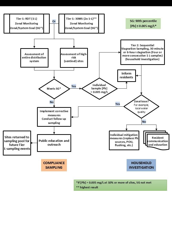
Figure A.4.1 - Text description
The flow chart has steps and decision points with yes or no questions for monitoring of residential dwellings, which is random daytime (RDT) and 30 minute stagnation (30 MS) (two-tier). The two tiers provide information on compliance sampling for the system goal (SG). Tier 2 provides information on household investigation sampling. The following information is presented in a box: the SG is that the 90th percentile lead concentration be less than or equal to 0.005 mg/L which means the lead concentration can be greater than 0.005 mg/L at less than 10% of sites.
Tier 1: RDT (1L) or 30MS (the highest result of 2x1L is retained), zonal monitoring, system goal (SG)
Simultaneous assessment of entire distribution system and high-risk (sentinel) sites
Question : Does the result meet the SG?
- If your answer is "Yes"
- For individual samples where the lead concentration is greater than 0.005 mg/L
- Inform residents of sample results
- Conduct Tier 2 sampling: Sequential stagnation sampling, 30 minute or 6-hour stagnation (Four or more consecutive 1 L samples). Household investigation
- For individual samples where the lead concentration is greater than 0.005 mg/L
Question: Is it a zonal issue (for example, local water quality)?
- If your answer is "Yes"
- Implement corrective measures, conduct follow-up sampling
- Conduct public education and outreach
- Return sites to sampling pool for future Tier 1 sampling events
- If your answer is "No"
- Implement individual mitigation measures (replace lead sources, POU, flushing, etc.)
- Undertake resident communication and education
- If your answer is "No" for meeting the SG
- Implement corrective measures, conduct follow-up sampling
- Conduct public education and outreach
- Return sites to sampling pool for future Tier 1 sampling events
A.4.2 Figure - Monitoring protocol for non-residential and multi-dwelling residential buildings (two-tier)
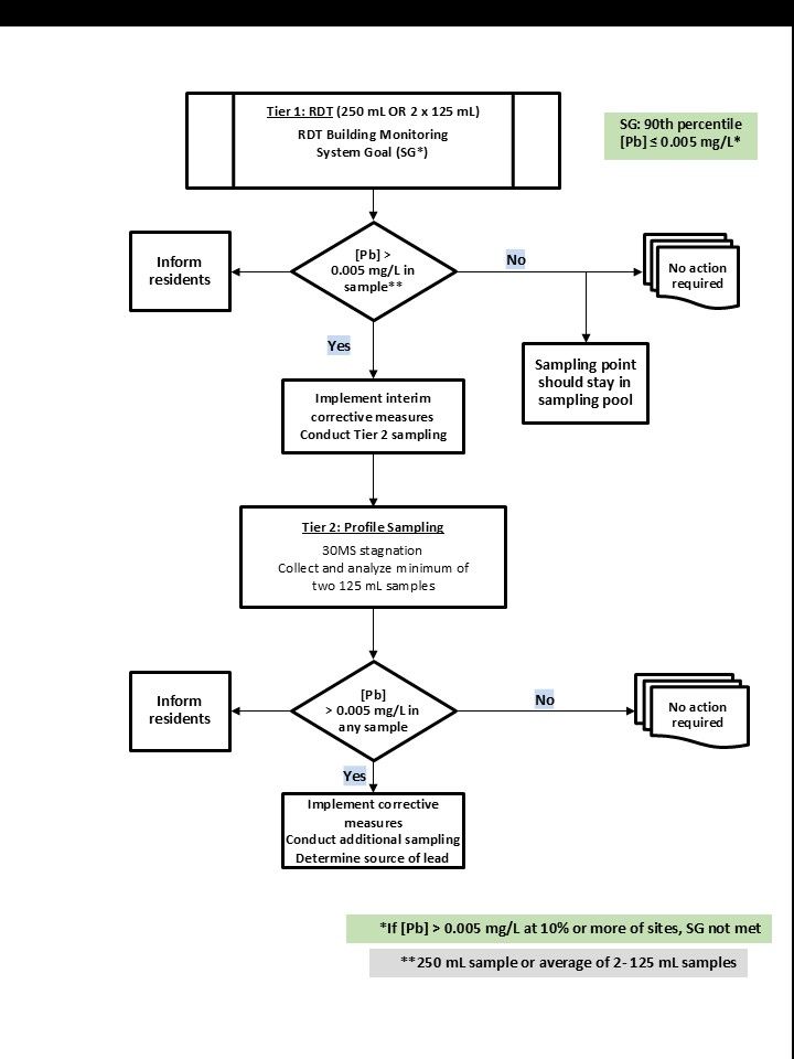
Figure A.4.2 - Text description
The flow chart has steps and decision points with yes or no questions for monitoring of non-residential and multi-dwelling residential buildings (two-tier). The following information is presented in a box: the system goal (SG) is that the 90th percentile lead concentration be less than or equal to 0.005 mg/L which means the lead concentration is greater than 0.005 mg/L at less than 10% of sites.
Tier 1: RDT (250 mL OR 2 x 125 mL). RDT building monitoring , system goal (SG)
Question: Is the lead concentration greater than 0.005 mg/L in any sample? Inform residents of sample results.
- If your answer is "Yes"
- Implement interim corrective measures.
- Conduct Tier 2 sampling.
- If your answer is "No"
- No action required.
- Sampling point should stay in sampling pool.
Tier 2: Profile sampling, 30 MS stagnation. Collect and analyze two 125 mL samples.
Question: Is lead concentration greater than 0.005 mg/L in any sample? Inform residents of sample results.
- If your answer is "Yes"
- Implement interim corrective measures.
- Conduct additional sampling.
- Determine source of lead.
- If your answer is "No"
- No action required.
Part B. Supporting information
B.1 Principles of corrosion in drinking water distribution systems
Exposure to contaminants resulting from the internal corrosion of drinking water systems can be the result of corrosion in either the distribution system or the plumbing system, or both.
Assessing the degree to which corrosion is controlled for a contaminant in a system can be adequately achieved by measuring the contaminant at the tap over time and correlating its concentrations with corrosion control activities.
This document focuses primarily on the corrosion of metallic materials. The emphasis is on the leaching of lead, but copper- and iron -based materials (including galvanized materials) are noted. Leaching from cement pipes is only briefly discussed. The document briefly discusses microbiologically influenced corrosion but does not include detailed information on the subject.
The corrosion of metallic materials is electrochemical in nature and is defined as the "destruction of a metal by electron transfer reactions" (Snoeyink and Wagner, 1996). For this type of corrosion to occur, all four components of an electrochemical cell must be present: (1) an anode, (2) a cathode, (3) a connection between the anode and the cathode for electron transport, and (4) an electrolyte solution that will conduct ions between the anode and the cathode. In the internal corrosion of drinking water distribution systems, the anode and the cathode are sites of different electrochemical potential on the metal surface, the electrical connection is the metal and the electrolyte is the water.
The key reaction in corrosion is the oxidation or anodic dissolution of the metal to produce metal ions and electrons:
M → Mn+ + ne−
where:
- M is the metal
- e is an electron
- n is the valence and the corresponding number of electrons.
In order for this anodic reaction to proceed, a second reaction must take place that uses the electrons produced. The most common electron acceptors in drinking water are dissolved oxygen and aqueous chlorine species.
The ions formed in the anodic reaction may be released into drinking water as corrosion products or may react with components present in the drinking water to form a scale on the surface of the pipe. The scale that forms on the surface of the metal may range from highly soluble and friable to adherent and protective. Protective scales are usually created when the metal cation combines with a hydroxide, oxide, carbonate, phosphate or silicate to form a precipitate.
The concentration of a specific metal in drinking water is determined by the corrosion rate and by the dissolution and precipitation properties of the scale formed. Initially, with bare metal, the corrosion rate far exceeds the dissolution rate, so a corrosion product layer builds over the metal's surface. As this layer tends to stifle corrosion, the corrosion rate drops towards the dissolution rate (Snoeyink and Wagner, 1996).
B.1.1 Primary contaminants from corrosion of drinking water distribution systems
The materials present in the distribution system determine which contaminants are most likely to be found at the tap. The primary contaminants of concern that can leach from corrosion of materials in drinking water distribution systems include antimony, cadmium, copper, iron, lead and zinc. It is important to assess whether these contaminants will be present at concentrations that exceed those considered safe for human consumption. Discolouration (red water) events are likely to be accompanied by the release of accumulated contaminants, including lead. Discoloured water should not be considered safe to consume or treated as only an aesthetic issue. Instead, the occurrence of discoloured water should trigger sampling for metals and potentially additional distribution system maintenance (Friedman et al., 2016).
B.1.2 Sources of contaminants in distribution systems
In Canada, widespread installation of lead service lines occurred until 1975. Many are still present owing to their durability. Copper plumbing with lead–tin solders (widely used until 1989) and brass faucets and fittings are predominant in domestic plumbing systems (Churchill et al., 2000).
Cast iron and ductile iron pipes have historically been used for water mains in Canada. The lining of ductile iron pipes and cast-iron mains with cement-mortar to make them resistant to corrosion remains a common practice (AWWA, 2017a). Galvanized steel was commonly used in plumbing pipes and well components for plumbing systems until 1980 (NRCC, 2015). Cement-based materials, including asbestos cement (A/C), are also commonly used to convey water in large-diameter pipes. In new installations, polyvinyl chloride (PVC) pipes often replace copper tubing, lead service lines and distribution pipes.
B.1.2.1 Lead pipes and solders
Lead was a common component of water distribution systems for many years. Lead may be found in, and leach into potable water from, pipes in old water mains, service lines, pipe jointing compounds and soldered joints, brass and bronze plumbing fittings, and goosenecks/pigtails, valve parts or gaskets used in water treatment plants or distribution mains.
Lead service lines have been shown to be a consistently high source of lead for many years and to contribute 50%–75% of the total lead at the tap after extended stagnation times (Sandvig et al., 2008). Lytle et al. (2019) collected sequential samples in Flint, Michigan during four sampling rounds from January to November 2016 to identify drinking water lead sources in homes. As part of this study, lead in drinking water was assessed before and after full lead service line removal at five locations. The authors found that full lead service line removal reduced the total mass of lead in drinking water by an average of 86%, confirming that lead service lines were the largest source of lead in homes.
Lead service lines have been shown to release lead in both dissolved and particulate form under various conditions (Health Canada, 2019a). A number of studies found iron release after full and partial lead service line replacement. These studies established a correlation between particulate lead at the tap and metals such as iron, zinc, tin and copper (Deshommes et al., 2010a; McFadden et al., 2011; Camara et al., 2013). More detailed information on lead release from lead service lines can be found elsewhere (Health Canada, 2019a).
All provinces, territories and lands under federal jurisdiction use the National Plumbing Code of Canada (NPC) as the basis for their plumbing regulations and/or policies. The NPC allowed lead as an acceptable material for pipes (service lines) until 1975 (NRCC, 2015).
The NPC officially prohibited lead solders from being used in new plumbing or in repairs to plumbing for drinking water supplies in the 1990 version (NRCC, 2015). The most common replacements for lead solders are tin–antimony, tin–copper and tin–silver solders. Under the NPC, components (that is, fittings) used for potable water applications must comply with the relevant standards for plumbing fittings (NRCC, 2015). The relevant standards, namely ASME A112.18.1/CSA B125.1 and CSA B125.3 (CSA, 2018a, 2018b), limit the lead content of solder to 0.2% and include requirements to comply with both NSF/ANSI/CAN Standard 61 and NSF/ANSI/CAN Standard 372 (NSF International, 2022a, 2022b).
Fixtures such as refrigerated water coolers and bubblers commonly used in schools and other non-residential buildings may contain lead. Selected components of water coolers such as soldered joints within the fixtures or the lining in the tank may contain alloys with lead (U.S. EPA, 2006). Some of these fixtures are still in use in Canada and can contribute high levels of lead to drinking water (McIlwain et al., 2015).
B.1.2.2 Copper pipes and brass fittings and fixtures
Copper is used in pipes and in copper alloys found in domestic plumbing. Copper alloys used in potable water systems are brasses (in domestic fittings) and bronzes (in domestic plumbing valves). Brasses are basically alloys of copper and zinc with other minor constituents, such as lead. Brass fittings are also often coated with a chromium–nickel compound. Bronzes (also referred to as red brass) are alloys of copper, tin and zinc, with or without lead. Historically, most brasses contained between 2% and 8% lead but generally contain less than 4% lead (NSF International, 2022a). A key strategy for reducing exposure to lead is to address leaching from these materials by specifying that they meet health-based and plumbing standards. A number of studies have demonstrated that the use of components such as faucets and other fittings with a low lead content can result in a reduced concentration of lead at the tap (Pieper et al., 2016; Health Canada, 2019a). NSF/ANSI/CAN Standard 61 (Drinking Water System Components—Health Effects) limits the leaching of lead into drinking water. To comply with NSF/ANSI/CAN Standard 372 (Drinking Water System Components—Lead Content) (NSF International, 2022a, 2022b), the lead content of components such as plumbing fittings and materials must not contain more than 0.25% lead as a weighted average.
Pieper et al. (2015) found that corrosion may be a significant concern for well owners and that brass components are the most likely source of lead. Another study found that lead leaching from lead brass (C36000) increased with decreasing pH and alkalinity (Pieper et al., 2016). More detailed information on lead release from brass can be found elsewhere (Health Canada, 2019a).
B.1.2.3 Iron pipes
The following iron-based materials are the principal sources of iron in drinking water distribution systems: cast iron, ductile iron, galvanized iron and steel. Iron may be released directly from iron-based materials or indirectly through the iron corrosion by-products, or tubercles, formed during the corrosion process, leading to discoloured (red) water events. Since cast iron and ductile iron are frequently found in Canadian drinking water distribution systems, it is not surprising that red water is the most common corrosion problem reported by consumers. When the iron concentration exceeds the aesthetic goal, the iron can stain laundry and plumbing fixtures, produce an undesirable taste in beverages and impart a yellow to red-brownish colour to the water.
Contaminants can accumulate within or on top of iron and lead corrosion products and scale deposits in distribution systems (Lytle et al., 2004; Schock, 2005; Schock et al., 2008a, 2014; Friedman et al., 2010). These scales can then be dislodged and released back to the water in the distribution system with accumulated contaminants such as lead and arsenic (Schock, 2005; U.S. EPA, 2006; Lytle et al., 2014). Iron release has also been correlated with particulate lead at the tap (Deshommes et al., 2010a; McFadden et al., 2011; Camara et al., 2013, Schock et al., 2014; Trueman and Gagnon, 2016; Trueman et al., 2017; Deshommes et al., 2017, 2018).
B.1.2.4 Galvanized pipes
Galvanized pipes will release zinc, since they are manufactured by dipping steel pipes in a bath of molten zinc. Galvanized pipes can also be sources of cadmium and lead, since these materials are present as impurities (Leroy et al., 1996).
The NPC permitted the use of galvanized steel as an acceptable material for pipes for plumbing systems until 1980 (NRCC, 2005). Lead and cadmium are correlated with zinc when galvanized steel pipes are the source of lead release (Clark et al., 2015). As such, the presence of cadmium may be an indicator that galvanized steel pipes are a source of lead. A study exposed brass and galvanized steel to more aggressive waters typically found in groundwaters. The study found that galvanized steel may still release significant lead as a result of the sorption of lead to plumbing. The authors concluded that galvanized steel would remain an issue for systems without corrosion control and that it is important for private well owners to test for lead (Pieper et al., 2016). More detailed information on lead and cadmium release from galvanized pipe can be found elsewhere (Health Canada, 2019a, 2020a).
Galvanized iron pipe and lead-lined galvanized iron pipe can also be significant contributors of lead in drinking water. Lead-lined pipes may be miscategorized as galvanized iron pipes when using commonly used methods for material identification. However, if the lead lining is intact, such pipes behave like a lead pipe and will release lead when subjected to the same conditions as a lead service line. The release of lead from galvanized iron pipes can be the result of chemical (for example, pH or alkalinity changes) or physical (for example, lead service line removal, water hammer or flow reversal) disturbances (Edwards et al., 2023). These factors highlight the importance of testing for lead when presumed galvanized iron pipes are present and during discoloured (red) water episodes.
B.1.2.5 Cement pipes
Cement-based materials used to convey drinking water include reinforced concrete pipes, cement-mortar linings and A/C pipes. In addition to the aggregates (sand, gravel or asbestos), which constitute the basic structure of cement, the binder, which is responsible for the cohesion and mechanical properties of the material, consists mostly of calcium silicates and calcium aluminates in varying proportions (Leroy et al., 1996). Degradation of cement-based materials causes substantial water quality degradation, especially in long lines or low-flow areas and with poor to moderately buffered waters. It can be a source of calcium hydroxide (lime) in the distributed water, which may result in an increase in pH and alkalinity. The degradation can also precipitate a variety of minerals, causing cloudy or turbid water and poor taste. In extreme cases, aggressive water can result in reduced pipe strength and cause increased head loss (Schock and Lytle, 2011).
The degradation of cement-based materials can also be a source of aluminum and asbestos in drinking water. The leaching of aluminum was observed in as little as 3 hours after the application of a cement-mortar lining inside a variety of pipe (steel, ductile iron) (Health Canada, 2021). Newly installed in situ mortar linings have been reported to cause water quality problems in dead ends or low-flow water conditions when water alkalinity is low (Douglas and Merrill, 1991).
B.1.2.6 Plastic pipes
PVC, polyethylene and chlorinated PVC pipes used in the distribution system have the potential to release contaminants into the distributed water. Stabilizers are used to protect PVC from decomposition when exposed to extreme heat during production. In Canada, organotin compounds are the most common stabilizers used in the production of PVC pipes for drinking water and can be released into drinking water. More detailed information on contaminant release from PVC pipes can be found elsewhere (Health Canada, 2013). Fittings intended for PVC pipes can be made of brass, which can be a potential source of lead where PVC pipes are used. Under the NPC, all plastic pipes must comply with the CSA B137 series of standards for plastic pipe, which require that pipes and the associated fittings comply with the NSF/ANSI/CAN Standard 61 (NSF International, 2022a) requirements for leaching of contaminants including contaminants such as organotin.
B.2 Challenges in measuring corrosion
There is no single, reliable index or method to measure water corrosivity and reflect population exposure to contaminants that are released by the distribution system. Given that a major source of metals in drinking water is related to corrosion in distribution and plumbing systems, measuring the contaminant at the tap is the best tool to assess corrosion and reflect population exposure.
B.2.1 Levels of contaminants at the tap
The literature indicates that lead, copper and iron are the contaminants whose levels are most likely to exceed guideline values owing to the corrosion of materials in drinking water distribution systems. The Guidelines for Canadian Drinking Water Quality establish MACs for lead (Health Canada, 2019a) and copper (Health Canada, 2019b), and an aesthetic objective for iron (Health Canada, 2024). The MAC for total lead is based on health considerations for the most sensitive population (children). Since a level under which lead is no longer associated with adverse health effects could not be identified, lead levels should be kept as low as reasonably achievable (Health Canada, 2019a). The guideline for copper is based on bottle-fed infants (Health Canada, 2019b) and the guideline for iron is based on an aesthetic objective (Health Canada, 2024). Both copper and iron are considered essential elements in humans at levels lower than their levels of concern. Based on these considerations and the recommendation to keep lead levels as low as reasonably achievable to minimize the potential for adverse health effects, lead concentrations at the tap are used as the basis for initiating corrosion control programs.
A national survey was conducted to ascertain the levels of cadmium, calcium, chromium, cobalt, copper, lead, magnesium, nickel and zinc in Canadian treated drinking water (Méranger et al., 1981). Based on the representative samples collected at the tap after 5 minutes of flushing at the maximum flow rate, the survey concluded that only copper levels significantly increased in the drinking water at the tap when compared with raw water.
Concurrently, several studies showed that concentrations of trace elements from household tap water sampled after a period of stagnation can exceed guideline values (Wong and Berrang, 1976; Lyon and Lenihan, 1977; Nielsen, 1983; Samuels and Méranger, 1984; Birden et al., 1985; Neff et al., 1987; Schock and Neff, 1988; Gardels and Sorg, 1989; Schock, 1990a; Singh and Mavinic, 1991; Lytle et al., 1993; Viraraghavan et al., 1996).
A number of contaminants can be accumulated in and released from the distribution system. Scales formed in distribution system pipes that have reached a dynamic equilibrium can subsequently release contaminants such as aluminum, arsenic, other trace metals and radionuclides (Valentine and Stearns, 1994; Reiber and Dostal, 2000; Lytle et al., 2004; Schock, 2005; Copeland et al., 2007; Morris and Lytle, 2007; Schock et al., 2008a; Friedman et al., 2010; Wasserstrom et al., 2017). Changes made to the treatment process, particularly those that affect water quality parameters such as pH, alkalinity and oxidation-reduction potential (ORP); blending; and change of water supply should be accompanied by close monitoring in the distributed water (Schock, 2005).
B.2.1.1 Lead service lines
Lead service lines have been shown to consistently be a high source of lead for many years and to contribute 50%–86% of the total lead at the tap after extended stagnation times (Sandvig et al., 2008; Lytle et al., 2019). Although the majority of lead released from lead service lines under stagnant conditions is dissolved lead, water flow can increase the release of both dissolved and particulate lead through the mass transfer of lead out of pipe scales and by physically dislodging the pipe scales. The relative contribution of lead in dissolved lead and particulate forms is not clearly understood and likely varies with water chemistry, plumbing configuration, stagnation time, flow regime, age of the plumbing materials containing the lead, and use patterns. Thus, sampling should be done at a medium to high flow rate as specified in A.2.6. The presence of particulate lead in drinking water is sporadic, unpredictable and often associated with mechanical disturbances to the system; it has been shown to also result from galvanic corrosion (Health Canada, 2019a) and to continue and even worsen over long periods of time (St. Clair et al., 2015).
Replacing the lead service line can disturb or dislodge existing lead scales or sediments containing lead, resulting in a significant increase in lead levels at the tap. This increase has been shown to continue for three or more months after the lead service line replacement (Health Canada, 2019a). Del Toral et al. (2013) found that disturbances to the lead service line increased lead concentrations in the water. These disturbances included meter installation or replacement, automated meter installation, service line leak or external service shut-off valve repair, and significant street excavation in proximity to the home.
Lead has been correlated with iron due to the adsorption of dissolved lead onto iron deposits in the lead service line and premise plumbing (Health Canada, 2019a; Trueman and Gagnon, 2016; Deshommes et al., 2017; Pieper et al., 2017, 2018; Trueman et al., 2017; Bae et al., 2020). Sustained lead release after full lead service line replacement can result from the adsorption of lead onto iron corrosion scales from old galvanized iron plumbing (McFadden et al., 2011; Edwards et al., 2023). The release of high levels of particulate lead for four years after full lead service line replacement was related to manganese and iron accumulation onto pipe walls of premise plumbing which provided a sink for lead. Manganese accumulation on lead pipes can obstruct the formation of the more stable lead(IV) corrosion scale, increasing the risk of lead release through more readily soluble scales (Schock et al., 2014).
Manganese and iron coatings occur often on lead and other types of pipes and can prolong the time it takes to build passivating films with corrosion inhibitors. They also tend to increase the risk of sporadic spikes of lead from particulate release. Manganese buildups throughout water distribution mains and storage are likely far more common than have been reported (Schock and Lytle, 2011).
Elevated lead levels were seen after both full and partial lead service line replacement and associated with iron released from a water supplied by an unlined iron distribution main (Camara et al., 2013; Trueman et al., 2017; Deshommes et al., 2017, 2018). Galvanized iron plumbing or iron deposits within premise plumbing can accumulate lead via adsorption, releasing it even after the primary source of lead has been removed (McFadden et al., 2011; Schock et al., 2014).
B.2.1.2 Lead-based solders
A study on the leaching of copper, iron, lead and zinc from copper plumbing systems with lead-based solders was conducted in the Greater Vancouver Regional District (Singh and Mavinic, 1991). The study showed that, for generally corrosive water (pH 5.5–6.3; alkalinity 0.6–3.7 mg/L as CaCO3), the first litre of tap water taken after an 8 hour period of stagnation exceeded the Canadian drinking water guidelines for lead and copper in 43% (lead) and 62% (copper) of the samples from high-rise buildings and in 47% (lead) and 73% (copper) of the samples from single-family homes. Even after prolonged flushing of the tap water in the high-rise buildings, there were still exceedances in 6% of the cases for lead and in 9% of the cases for copper. In all cases in the single -family homes, flushing the cold water for 5 minutes reduced levels of lead and copper below the guideline levels.
Subramanian et al. (1995) examined the leaching of antimony, cadmium, copper, lead, silver, tin and zinc from new copper piping with non-lead-based soldered joints exposed to different waters qualities (pH 7.5–8.4; alkalinity 40–150 mg/L as CaCO3) over a 28-day period to evaluate the leaching over stagnation times ranging from 1 hour to 672 hours. All lead concentrations exceeded 5 µg/L in as little as 1 hour under all water quality conditions and generally increased with time. The authors concluded that 50:50 lead–tin solders used in copper pipes increasingly leached lead into drinking water in samples for up to 28 days.
Lead solder can also be a source of particulate lead that is subsequently trapped in the tap aerator. These particulates can result in significant lead concentrations at the tap. More detailed information on particulate lead release can be found elsewhere (Health Canada, 2019a).
B.2.1.3 Faucets and brasses
Samuels and Méranger (1984) conducted a study on the leaching of trace metals from kitchen faucets in contact with the City of Ottawa's water (pH 6.3–8.1). Water was collected after a 24-hour period of stagnation in new faucets not washed prior to testing. In general, the concentrations of cadmium, chromium, copper and zinc in the leachates did not exceed the Canadian drinking water guideline values applicable at that time. However, levels well above the guideline value for lead were leached from the faucets containing lead-soldered copper joints.
Similar work by Schock and Neff (1988) revealed that new chrome-plated brass faucets can be a significant source of copper, lead and zinc contamination of drinking water, particularly upon stagnation of the water. The authors also concluded that faucets, as well as other brass fittings in household systems, provide a continuous source of lead, even when lead-free solders and fluxes are used in copper plumbing systems. Maas et al. (1994) conducted a statistical analysis of water samples collected in non-residential buildings after an overnight stagnation period from over 12 000 water fountains, bubblers, chillers, faucets and ice makers. The analysis indicated that over 17% of the samples had lead concentrations above 15 µg/L. Notably, the drinking water collected from bubblers, chillers and faucets had lead concentrations above 15 µg/L in over 25% of the samples. Other studies found that between 5% and 21% of drinking water fountains or faucets had lead concentrations above 20 µg/L following a period of stagnation greater than 8 hours (Gnaedinger, 1993; Bryant, 2004; Sathyanarayana et al., 2006; Boyd et al., 2008a).
Studies conducted in Copenhagen, Denmark found that nickel was leaching from chromium-nickel–plated brass after periods of water stagnation (Anderson, 1983). Nickel concentrations measured in the first 250 mL ranged from 8 to 115 µg/L and dropped to 9 to 19 µg/L after 5 minutes of flushing. Similarly, large concentrations of nickel (up to 8 700 µg/L in one case) were released from newly installed chromium-nickel–plated brass, nickel-plated parts and nickel-containing gunmetal following 12-hour periods of water stagnation (Nielsen and Andersen, 2001). Kimbrough (2001) found that brass was a potential source of nickel at the tap. Nickel was found in the first litre after a period of water stagnation (mean and maximum concentrations ranged from 4.5–9.2 µg/L and from 48–102 µg/L, respectively) with the results also indicating that almost all of the nickel was contained in the first 100 mL.
B.2.1.4 Iron pipes
When iron pipes, including galvanized iron pipes, are exposed to aerated or chlorinated water, metallic iron is oxidized and iron corrosion products form (for example, tubercles). Although the dominant oxidant in most water supplies is dissolved oxygen, chlorine also increases the corrosion rate; however, concentrations are typically lower than that of dissolved oxygen. The iron corrosion rate depends on the dissolved oxygen concentration and on its transported rate to the metal surface. The ferrous ions produced by the oxidation reactions may either dissolve in the water or deposit on the corroded iron surface as a scale. The growth of the scale decreases the iron corrosion rate but the dissolution of the corrosion by-products contributes to iron release in the water. The extent to which this process occurs depends on the water quality and hydraulic conditions (Benjamin et al., 1996; McNeill and Edwards, 2001; Edwards et al., 2023). Water flow in the pipe, temperature, thickness and the porosity of the accumulated scale on the metal surface affect the oxygen transport. Water quality parameters such as alkalinity, pH and the concentration of inorganic ions have a minimal effect on the corrosion rate; however, they may influence corrosion scale formation and, subsequently, the corrosion rate at a later stage (Benjamin et al., 1996).
Many studies have shown that iron scales can act as a sink for, and persistent source of, lead in drinking water (Friedman et al., 2010; Schock et al., 2014). In particular, iron concentrations at the tap have been correlated with lead. Elevated lead levels were seen after both full and partial lead service line replacement and were associated with iron release from a water supplied by an unlined iron distribution main (Camara et al., 2013; Trueman and Gagnon, 2016; Deshommes et al., 2017; Pieper et al., 2017, 2018; Trueman et al., 2017; Health Canada, 2019a). Galvanized iron plumbing or iron deposits within premise plumbing can accumulate lead via adsorption, releasing it even after the primary source of lead has been removed (McFadden et al., 2011; Schock et al., 2014; Edwards et al., 2023).
Iron hydroxides may also adsorb and concentrate other contaminants, including manganese, arsenic and aluminum. The installation of chlorination at a groundwater system in the U.S. caused exceptionally high arsenic concentrations at the tap. Chlorination induced the formation of ferric hydroxide solids, which readily sorbed and concentrated arsenic present in the groundwater at concentrations below 10 µg/L. The addition of chlorine also resulted in the release of copper oxides, which in turn sorbed and concentrated arsenic. Arsenic concentrations as high as 5 mg/L were found in the water samples collected (Reiber and Dostal, 2000). Triantafyllidou et al. (2019) reported average arsenic levels at the tap ranging from 0.5 to 51 μg/L in systems where elevated levels were attributed in part to desorption from dissolution of or resuspension along with iron oxides. Manganese, cadmium, chromium, barium, radium, thorium and uranium have been detected along with iron in hydrant flush solids. Manganese has been shown to accumulate in loose deposits of distribution pipe materials, including iron pipes, where it is associated with tubercle deposits (Health Canada, 2019d). Manganese has been found to accumulate to a lesser extent in iron pipe surface scale than in PVC pipes (Imran et al., 2005; Friedman et al., 2016). Aluminum can accumulate on iron pipes and be released, along with other contaminants, when water quality changes. Physical/hydraulic disturbances may also cause aluminum deposits to detach (Health Canada, 2021).
Furthermore, the scale may later be released if the quality of the water distributed is modified (Reiber and Dostal, 2000; Lytle et al., 2004) or if there are changes to the hydraulic conditions. Water supply changes may also yield red water events and a concomitant increase in concentrations of inorganic contaminants. (Friedman et al., 2016).
Iron corrosion products in the distribution system support microbial growth, and corrosion scale provides a favourable habitat for microbes, as do suspended corrosion products. Corrosion releases ferrous iron, which is oxidized by chlorine to ferric iron, depleting the disinfectant residual and enabling microbial growth. Sulphate reducers, nitrate reducers, nitrate oxidizers, ammonia oxidizers, sulphur oxidizers and unidentified heterotrophic microorganisms have been detected in iron tubercles (Tuovinen et al., 1980). A number of coliform species were detected in iron tubercles (Emde et al., 1992; LeChevallier et al., 1988). Tubercles can also harbour opportunistic pathogens such as Legionella (NASEM, 2020; Health Canada, 2022). Corroded iron provides sites for bacterial growth, thereby protecting biofilm bacteria from inactivation by free chlorine. Even low levels of iron corrosion (such as 1 mm/yr) support greater bacterial biomass than uncorroded pipe. Higher corrosion rates also diminish the disinfection capacity of monochloramine (LeChevallier et al., 1993).
B.2.1.5 Cement pipes
High concentrations of aluminum were found in the drinking water of Willemstad, Curaçao, Netherlands, Antilles, following the installation of 2.2 km of new cement-lined ductile iron pipes with a high aluminum content (18.7% as aluminum oxide) (Berend and Trouwborst, 1999). Aluminum concentrations in the distributed water increased from 5 µg/L to 690 µg/L within 2 months of installation and were still above 100 µg/L after 2 years. These atypical, elevated aluminum concentrations were attributed to the low hardness (15–20 mg/L as CaCO3), low alkalinity (18 –32 mg/L as CaCO3), high pH (8.5–9.5) and long contact time (2.3 days) of the distributed water and the use of polyphosphate as a corrosion inhibitor.
Aluminum was also found to leach from in situ Portland cement–lined pipes in a series of field trials carried out throughout the United Kingdom in areas with different water qualities (Conroy, 1991). Aluminum concentrations above the European Community (EC) Directive of 0.2 mg/L were found following installation in very low-alkalinity water (around 10 mg/L as CaCO3) with elevated pH (> 9.5) and contact times of 6 hours. Aluminum concentrations dropped below 0.2 mg/L after 2 months of pipe service. Furthermore, in water with slightly higher alkalinity (~ 50 mg/L as CaCO3), aluminum was not found to exceed the EC Directive. The Canadian guideline value for aluminum in drinking water is a MAC of 2.9 mg/L and is based on neurological effects (Health Canada, 2021).
Asbestos fibres have been found to be released from A/C pipes (Leroy et al., 1996; WHO, 2021). Release of asbestos fibres from A/C pipes is related to the quality of the water supply, including pH, hardness (calcium and carbonate), and the presence of constituents such as silica, iron, manganese and zinc (Buelow et al., 1980; Schock & Buelow, 1981). This can be mitigated by coating the inside of the distribution pipes. A study concluded that failure of A/C pipes was associated with low pH, low alkalinity, age and whether the internal surface of the pipe was protected with coal tar, bitumen or epoxy resin (Mordak & Wheeler, 1988). There is no MAC for asbestos in drinking water (Health Canada, 1989) as there is no consistent, convincing evidence that ingested asbestos is hazardous. In 2021, the World Health Organization concluded that the overall weight of evidence did not suggest an increased risk of cancer following ingestion of asbestos in drinking water. It was not considered appropriate or necessary to establish a guideline value for asbestos fibres in drinking water (WHO, 2022a).
B.2.2 Factors influencing levels of contaminants at the tap
Many factors contribute to the corrosion and leaching of contaminants from drinking water distribution systems. However, the principal factors are the type of materials used, the age of the plumbing system, the stagnation time of the water and the quality of the water in the system. The concentrations of all corrosive or dissolvable materials present in the distribution system will be influenced to varying degrees by some or all of these factors.
Microbiologically influenced corrosion results from a reaction between the pipe material and organisms, their metabolic by-products or both (Schock and Lytle, 2011). Microbial activity can affect pH, metal solubility and the oxidation-reduction potential of the surrounding microenvironment. More detailed information on this type of corrosion can be found in other reference documents (AWWA, 2017a; Health Canada, 2019b).
Factors influencing the corrosion and leaching of lead, copper, iron (including galvanized iron) and cement are discussed here, since these materials are most likely to produce contaminants that exceed Canadian drinking water guidelines, pose health risks to the public or be a source of consumer complaints.
B.2.2.1 Age of the plumbing system
Lead concentrations at the tap originating from lead solders and brass fittings decline with age (Sharrett et al., 1982; Birden et al., 1985; Boffardi, 1988, 1990; Schock and Neff, 1988; Neuman, 1995). Researchers concluded that the highest lead concentrations appeared in the first year following installation and level off after a number of years of service (Sharrett et al., 1982; Boffardi, 1988). However, unlike lead-soldered joints and brass fittings, lead piping can continue to provide a consistently strong source of lead after many years of service (Britton and Richards, 1981; Schock et al., 1996). In a field study in which lead was sampled in tap water, Maas et al. (1991) showed that homes of all ages were at a substantial risk of lead contamination.
The age of the plumbing materials, fittings and devices is particularly important for copper and brasses (Schock and Lytle, 2011). Copper release into the drinking water largely depends on the type of scale formed within the plumbing system. It can be assumed that, at a given age, a corrosion by-product governs the release of copper into the drinking water. A decrease in solubility in the following order is observed based on the predominating scales: cuprous hydroxide [Cu(OH)2] > bronchantite [Cu4(SO4)(OH)6] >> cupric phosphate [Cu3(PO4)2] > tenorite [CuO] and malachite [Cu2(OH)2CO3] (Schock et al., 1995). Copper concentrations continue to decrease with the increasing age of plumbing materials, even after 10 or 20 years of service, when tenorite or malachite scales tend to predominate (Sharrett et al., 1982; Neuman, 1995; Edwards and McNeill, 2002). In certain cases (for example, alkalinity of 300 mg/L as CaCO3 in older pipe), sulphate and phosphate can at first decrease copper concentrations by forming bronchantite and cupric phosphate, but in the long run they may prevent the formation of the more stable tenorite and malachite scales (Edwards et al., 2002).
The age of an iron pipe affects its corrosion. In general, both iron concentration and the rate of corrosion increase with time when a pipe is first exposed to water, but both are then gradually reduced as the scale builds up (McNeill and Edwards, 2001). However, most red water problems today are caused by old, heavily tuberculated unlined cast iron pipes that are subject to stagnant water conditions prevalent in dead ends. Sarin et al. (2003) removed unlined cast iron pipes that were 90–100 years old from distribution systems and found that the internal surface had up to 76% of the cross-section of the pipes blocked by scales. Such pipes are easily subject to scouring and provide the high surface areas that favour the release of iron.
A newly installed cement-based material will typically leach lime, which in turn will increase water pH, alkalinity and concentrations of calcium (Holtschulte and Schock, 1985; Douglas and Merrill, 1991; Conroy et al., 1994; Douglas et al., 1996; Leroy et al., 1996).
Experiments by Douglas and Merrill (1991) showed that, after 1, 6 and 12 years in low-flow, low-alkalinity water, lime continued to leach from cement mortar linings upon prolonged exposure, but at a significantly decreased rate when comparing 6- and 12-year-old pipes with the 1-year-old pipe. The lime leaching rate naturally slows down as surface calcium becomes depleted and the deposits formed over time may protect the mortar against further leaching.
B.2.2.2 Stagnation time, water age and flow
Lead
Concentrations of lead and copper in drinking water from various sources of lead material, including lead service lines, lead solder and brass fittings that contain lead, can increase significantly following a period of water stagnation of a few hours in the distribution system. Many factors, such as the water quality and the age, composition, diameter and length of the lead pipe impact the shape of stagnation curves and the time to reach an equilibrium state (Lytle and Schock, 2000).
In reviewing lead stagnation curves drawn by several authors, Schock et al. (1996) concluded that lead levels increase exponentially upon stagnation, but ultimately approach a fairly constant equilibrium value after overnight stagnation. Lytle and Schock (2000) showed that lead levels increased rapidly with the stagnation time of the water, with the most critical period being during the first 20–24 hours for both lead pipe and brass fittings. Lead levels increased most rapidly over the first 10 hours, reaching approximately 50%–70% of the maximum observed value. In their experiment, lead levels continued to increase slightly even up to 90 hours of stagnation.
Kuch and Wagner (1983) plotted lead concentrations versus stagnation time for two different water qualities and lead pipe diameters. The lead concentrations in 1/2-inch (1.3-cm) pipe where the pH of the water was 6.8 and the alkalinity was 10 mg/L as CaCO3 were significantly higher than lead concentrations stagnating in 3/8-inch (0.95-cm) pipe where the pH of the water was 7.2 and the alkalinity was 213 mg/L as CaCO3. Additional data from Kuch and Wagner (1983) indicate that lead levels approach maximum or equilibrium concentrations at greater than 300 minutes (5 hours) for 1/2-inch pipe (1.3-cm lead service line) and at greater than 400 minutes (6.7 hours) for 3/8-inch (1.0-cm) pipe. The diameter of pipes or lead service lines in Canada ranges from 1/2-inch (1.3-cm) to 3/4-inch (1.9-cm) but is typically 5/8-inch (1.6-cm) to 3/4-inch (1.9-cm). Lead concentrations have been demonstrated to be highly sensitive to stagnation time in the first 3 hours of standing time for 1/2-inch (1.3-cm) to 3/4-inch (1.9-cm) pipe. Depending on the water quality characteristics and pipe diameters, differences in lead concentration between 10% and 30% could be observed with differences in standing time as little as 30–60 minutes (Kuch and Wagner, 1983; Schock, 1990a). Long lead or copper pipe of small diameter produces the greatest concentrations of lead or copper, respectively, upon stagnation (Kuch and Wagner, 1983; Ferguson et al., 1996).
Lead is also released during no-flow periods from soldered joints and brass fittings (Birden et al., 1985; Neff et al., 1987; Schock and Neff, 1988). Wong and Berrang (1976) concluded that lead concentrations in water sampled in a 1-year-old household plumbing system made of copper with tin–lead solders could exceed 0.05 mg/L after 4–20 hours of stagnation and that lead concentrations in water in contact with lead water pipes could exceed this value in 10 to 100 minutes. In a study examining the impact of stagnation time on lead release from brass coupons, Schock et al. (1995) observed that, for brass containing 6% lead, lead concentrations increased slowly for the first hour. Following a 6-hour stagnation period, the lead concentration was greater than 0.04 mg/L, but ultimately reached a maximum concentration of 0.08 mg/L following 15 hours of stagnation. The amount of lead released from brass fittings was found to vary with both alloy composition and stagnation time.
Stagnation times, flow regime and water chemistry have been shown to influence the release of particulate lead from lead service line scales. Particulate lead has been observed to increase under flowing and stagnant water conditions as well as low-flow conditions, in the presence of orthophosphate, with increasing stagnation time and at higher pH under flowing water conditions. Of particular interest is that studies have consistently shown that moderate to high flow rates (> 5 L/minute) typical of turbulent flow or flow disturbances can increase the mobilization of lead and result in significant contributions of particulate lead to the total lead concentration (Health Canada, 2019a).
Copper
Copper behaviour is more complex than that of lead when it comes to water stagnation. Copper levels will initially increase upon stagnation of the water, but can then decrease or continue to increase, depending on the oxidant levels. Lytle and Schock (2000) showed that copper levels increased rapidly with the stagnation time of the water, but only until dissolved oxygen fell below 1 mg/L, after which they dropped significantly. This is further demonstrated in a study on the influence of stagnation and temperature on water quality in distribution systems (Zlatanovic et al., 2017). The authors found that concentrations of copper increased with stagnation time during winter and summer. Copper levels peaked at 1 370 mg/L after 48 hours of stagnation during winter and 1 140 mg/L after 24 hours of stagnation during summer, when both were sampled at the tap. Copper levels decreased after the peak for both seasons (pH and alkalinity not provided). Sorg et al. (1999) also observed that, in softened water, copper concentrations increased to maximum levels of 4.4 mg/L and 6.8 mg/L after about 20–25 hours of standing time, then dropped to 0.5 mg/L after 72–92 hours. Peak concentrations corresponded to the time when the dissolved oxygen was reduced to 1 mg/L or less. In non-softened water, the maximum was reached in less than 8 hours because the dissolved oxygen decreased more rapidly in the pipe loop exposed to non-softened water. High-flow velocities can sometimes be associated with erosion corrosion or the mechanical removal of the protective scale in copper pipes. Water flowing at high velocity, combined with corrosive water quality, can rapidly deteriorate pipe materials (Health Canada, 2019b).
Iron
Most red water issues are caused by old, heavily tuberculated unlined cast iron pipes that are subject to stagnant water conditions prevalent in dead ends. Cyclic periods of flow and stagnation were reported as the primary cause of red water problems resulting from iron corrosion of distribution systems (Benjamin et al., 1996). Iron concentration was also shown to increase with longer water stagnation time prevalent in dead ends (Beckett et al., 1998; Sarin et al., 2000). Iron corrosion can also occur in a water supply under conditions where there is limited dissolved oxygen (stagnant water). During stagnation, the dissolved oxygen concentration is depleted near the metal surface and ferric oxides in the corrosion scale may serve as the alternative oxidant. Under these conditions, ferric iron serves as the oxidant and ferrous iron is generated. Ferrous iron may precipitate or diffuse into the distributed water and is then oxidized to (insoluble) ferric iron by the dissolved oxygen, contributing to red water (Benjamin et al., 1996; Sarin et al., 2004 a, b). Red water complaints may occur when cyclic periods of flow and stagnation in water occur (Benjamin, 1996).
Cement
Long contact time between distributed water and cement materials has been correlated with increased water quality deterioration (Holtschulte and Schock, 1985; Conroy, 1991; Douglas and Merrill, 1991; Conroy et al., 1994; Douglas et al., 1996; Berend and Trouwborst, 1999). In a survey of 33 U.S. utilities with newly installed in situ lined cement mortar pipes carrying low-alkalinity water, Douglas and Merrill (1991) concluded that degraded water quality was most noticeable in dead ends or where the flow was low or intermittent. Similarly, Conroy (1991) and Conroy et al. (1994) found that the longer the supply water was in contact with the mortar lining, the greater the buildup of leached hydroxides, and hence the higher the pH.
B.2.2.3 pH
The effect of pH on the solubility of the corrosion by-products formed during the corrosion process is often the key to understanding the concentration of metals at the tap. An important characteristic of distributed water with higher pH is that the solubility of the corrosion by-products formed in the distribution system typically decreases. However, these effects are not universal as some metals (and/or species of metals) are released with a pH decrease (for example, lead, copper and manganese) but they can also be released in response to a pH increase (for example, arsenic, copper, chromium) (Kim et al., 2011; Wahman et al., 2021). The release of metals from materials used in distribution and premise piping systems will not only be affected by pH, but also by the alkalinity and DIC levels of the water, as they influence the formation of the passivating scale on the surface of the material. The presence of these passivating scales on internal pipe surfaces will help prevent the release of lead or copper to the water (Schock and Lytle, 2011).
Lead
The passivation of lead usually results from the formation of a surface film composed of a lead(II) hydroxycarbonate or orthophosphate solids. The solubility of the main divalent lead corrosion by-products cerussite [PbCO3], hydrocerussite [Pb3(CO3)2(OH)2] and lead hydroxide [Pb(OH)2]) largely determines the lead levels at the tap (Schock, 1980, 1990b; Sheiham and Jackson, 1981; De Mora and Harrison, 1984; Boffardi, 1988, 1990; U.S. EPA, 1992; Leroy, 1993; Peters et al., 1999).
From thermodynamic considerations, lead solubility of corrosion by-products in distribution systems decreases with increasing pH (Britton and Richards, 1981; Schock and Gardels, 1983; De Mora and Harrison, 1984; Boffardi, 1988; Schock, 1989; U.S. EPA, 1992; Singley, 1994; Schock et al., 1996). Solubility models based on lead(II) chemistry show that the lowest lead levels occur when pH is around 9.8. However, these pH relationships may not be valid for insoluble tetravalent lead dioxide (PbO2) solids, which have been found in lead pipe deposits from several different water systems with high oxidation-reduction potential (highly oxidizing conditions) (Schock et al., 1996, 2001; Schock and Lytle, 2011). Depending on the pH and alkalinity of the water, pipe scales may include hydrocerrusite (low pH, low alkalinity), cerussite and massicot (PbO) (higher alkalinity) (McNeill and Edwards, 2004).
Lead dioxide has been found to be present in waters of low pH and frequently in waters with high alkalinity (Schock et al., 2001, 2005b). Based on tabulated thermodynamic data, the pH relationship of PbO2 may be opposite to that of divalent lead solids (for example, cerussite, hydrocerrussite) (Schock et al., 2001; Schock and Giani, 2004). Lytle and Schock (2005) demonstrated that PbO2 easily formed at pH 6–6.5 in water with persistent free chlorine residual in weeks to months.
Release of lead from lead solder is primarily controlled by galvanic corrosion and increasing pH has been associated with a decrease in corrosion of lead solder (Oliphant, 1983a; Schock and Lytle, 2011).
Municipality experience has also shown that the lowest levels of lead at the tap are associated with pH levels above 8 (Karalekas et al., 1983; Lee et al., 1989; Dodrill and Edwards, 1995; Douglas et al., 2004). Based on bench- and pilot-scale experimental results and analysis of several criteria, the City of Ottawa selected a pH of 9.2 and a minimum alkalinity target of 35 mg/L as CaCO3, using sodium hydroxide and carbon dioxide, to control corrosion. During the initial switch to sodium hydroxide, the pH was maintained at 8.5. However, lead testing found an area of the city with high levels of lead at the tap (10–15 µg/L for flowing samples). Nitrification in the distribution system caused the pH to decrease from 8.5 to a range of 7.8–8.2 and resulted in lead release from lead service lines. Increasing the pH to 9.2 resulted in an almost immediate reduction in lead concentrations ranging from 6– 8 µg/L for flowing samples. Ongoing monitoring has demonstrated that lead levels at the tap, following the increase in pH, were consistently below the regulated level of 10 µg/L (1.3 to 6.8 µg/L) (Douglas et al., 2007).
Examination of treatment system data provided by 365 utilities revealed that the average 90th percentile lead levels at the tap were dependent on both pH and alkalinity (Dodrill and Edwards, 1995). In the lowest pH category (pH < 7.4) and lowest alkalinity category (alkalinity < 30 mg/L as CaCO3), utilities had an 80% likelihood of exceeding the U.S. EPA Lead and Copper Rule Action level for lead of 0.015 mg/L. In this low-alkalinity category, only a pH greater than 8.4 seemed to reduce lead levels at the tap. However, when an alkalinity greater than 30 mg/L as CaCO3 was combined with a pH greater than 7.4, the water produced could, in certain cases, meet the Action level for lead.
A survey of 94 water utilities sampling a total of 1 484 sites, with both non-lead and lead service lines, after an overnight stagnation of at least 6 hours was conducted to evaluate the factors that influence lead levels at the consumer's tap (Lee et al., 1989). The authors demonstrated that maintaining a pH of at least 8.0 effectively controlled lead levels (< 10 µg/L) in the first litre collected at the tap.
A 5-year study to reduce lead concentrations in the drinking water distribution system of the Boston, Massachusetts metropolitan area was conducted (Karalekas et al., 1983). Fourteen households were examined for lead concentrations at the tap, in their lead service lines and in their adjoining distribution systems. Average concentrations were reported for combined samples taken (1) after overnight stagnation at the tap, (2) after the water turned cold and (3) after the system was flushed for an additional 3 minutes. Even if alkalinity remained very low (on average 12 mg/L as CaCO3), raising the pH from 6.7 to 8.5 reduced average lead concentrations from 0.128 mg/L to 0.035 mg/L.
Copper
Although the hydrogen ion does not play a direct reduction role on copper surfaces, pH can influence copper corrosion by altering the equilibrium potential of the oxygen reduction half-reaction and by changing the speciation of copper in solution (Reiber, 1989). The release of copper is highly pH dependent. When copper corrodes, it is oxidized to Cu(I)(cuprous) and Cu(II)(cupric) copper species that may form protective copper carbonate-based (passivating) scales on the surface of copper plumbing materials, depending on the pH and the levels of DIC and oxidizing agents in the water (Atlas et al., 1982; Pisigan and Singley, 1987; Schock et al., 1995; Ferguson et al., 1996). Copper corrosion increases rapidly as the pH drops below 6; in addition, uniform corrosion rates can be high at low pH values (below about pH 7), causing metal thinning. At higher pH values (above about pH 8), copper corrosion problems are almost always associated with non-uniform or pitting corrosion processes (Edwards et al., 1994a; Ferguson et al., 1996). Edwards et al. (1994b) found that, for new copper surfaces exposed to simple solutions that contained bicarbonate, chloride, nitrate, perchlorate or sulphate, increasing the pH from 5.5 to 7.0 roughly halved corrosion rates but further increases in pH yielded only subtle changes.
The prediction of copper levels in drinking water relies on the solubility and physical properties of the cupric oxide, hydroxide and basic carbonate solids that comprise most scales in copper water systems (Schock et al., 1995). In the cupric hydroxide model of Schock et al. (1995), a decrease in copper solubility with higher pH is evident. Above a pH of approximately 9.5, an upturn in solubility is predicted, caused by carbonate and hydroxide complexes increasing the solubility of cupric hydroxide. Examination of experience from 361 utilities reporting copper levels revealed that the average 90th percentile copper levels were highest in waters with a pH below 7.4 and that no utilities with a pH above 7.8 exceeded the U.S. EPA's Action level for copper of 1.3 mg/L (Dodrill and Edwards, 1995). However, problems associated with copper solubility were also found to persist up to about pH 7.9 in cold, high-alkalinity and high-sulphate groundwater (Edwards et al., 1994a).
In general, copper solubility increases (that is, copper levels will increase) with increasing DIC and decreasing pH (Schock, et al., 1995; Ferguson, et al., 1996). Copper levels may be controlled at lower pH levels. However, high-alkalinity, high-DIC groundwaters are prone to copper corrosion problems and adjusting pH may be impractical because of the potential for CaCO3 precipitation.
Iron
Release of iron from iron-based drinking water materials, such as cast iron, steel and ductile iron, has been modelled based on the formation of protective ferrous solid scales (FeCO3). In the pH range of 7–9, both the corrosion rate and the degree of tuberculation of iron distribution systems generally increase with increasing pH (Larson and Skold, 1958; Stumm, 1960; Hatch, 1969; Pisigan and Singley, 1987). However, the solubility of iron-based corrosion by-products, and thus iron levels, decrease with increasing pH (Karalekas et al., 1983; Kashinkunti et al., 1999; Broo et al., 2001; Sarin et al., 2003). In a pipe loop system constructed from 90- to 100-year-old unlined cast iron pipes taken from a Boston distribution system, iron concentrations were found to steadily decrease when the pH was raised from 7.6 to 9.5 (Sarin et al., 2003). Similarly, following a pH increase from 6.7 to 8.5, a consistent downward trend in distribution system iron concentrations was found over 2 years (Karalekas et al., 1983). The rate of ferrous iron oxidation increases with pH and, generally, both the solubility and dissolution rates of iron oxides—and other iron compounds—decrease with increasing pH (Schwertmann, 1991; Sarin et al., 2003; Duckworth & Martin, 2004). Finished water pH was lowered from 10.3 to 9.7, resulting in reduced soluble lead release. However, iron concentrations were found to increase at pH 9.7 and were correlated with increased particulate lead release (Masters and Edwards, 2015).
Waters with high buffer intensity will mitigate changes in pH, and a relatively stable pH will encourage the formation of the more protective ferrous-based solids and result in lower iron release. Maintaining a stable pH can be important for preventing desorption of inorganic contaminants from iron oxides.
Cement
Water with low pH, low alkalinity and low calcium is particularly aggressive towards cement materials. The water quality problems that may occur are linked to the chemistry of the cement. Lime from the cement releases calcium ions and hydroxyl ions into the drinking water. This, in turn, may result in a substantial pH increase, depending on the water's buffering capacity (Leroy et al., 1996). Pilot-scale tests were conducted to simulate low-flow conditions of newly lined cement mortar pipes carrying low-alkalinity water (Douglas et al., 1996). In the water with an initial pH of 7.2, alkalinity of 14 mg/L as CaCO3 and calcium at 13 mg/L as CaCO3, measures of pH as high as 12.5 were found. Similarly, in the water with an initial pH of 7.8, alkalinity of 71 mg/L as CaCO3 and calcium at 39 mg/L as CaCO3, measures of pH as high as 12 were found. The most significant pH increases were found during the first week of the experiment and pH decreased slowly as the lining aged. In a series of field and test rig trials to determine the impact of in situ cement mortar lining on water quality, Conroy et al. (1994) observed that in low-flow and low-alkalinity water (around 10 mg/L as CaCO3), pH increases exceeding 9.5 could occur for over 2 years following the lining. A/C pipes are particularly susceptible to low-pH waters (less than 7.5–8.0) with high calcium alkalinity and silicate levels (Schock and Lytle, 2011).
Field trials carried out throughout the United Kingdom in areas with different water qualities found that high pH in cement pipes can render lead soluble. Lead levels increased significantly with increasing pH when pH was above 10.5. The concentration of lead ranged from just less than 100 µg/L at pH 11 to greater than 1 000 µg/L above pH 12 (Conroy, 1991). This brings into question the accuracy of the solubility models for high pH ranges and the point at which pH adjustment may become detrimental. Elevated pH levels resulting from cement leaching may also contribute to aluminum leaching from cement materials, since high pH may increase aluminum solubility (Berend and Trouwborst, 1999). Aluminum can interfere with orthophosphate passivation used for corrosion control by preventing the formation of protective scales (AWWA, 2017a; Wasserstrom et al., 2017).
Zinc
Zinc coatings on galvanized steel corrode similarly to iron but the corrosion reactions are typically slower. Corrosion of the galvanized pipes can release trace metals, such as cadmium and lead, into drinking water distribution systems. When the pipe is new, corrosion depends strongly on pH. Pisigan and Singley (1987) found that, below pH 7.5, zinc levels increased in drinking water (DIC concentration of 50 mg of carbon/litre (C/L)). At pH levels of 7.5–10.4, hydrozincite, the most stable corrosion by-product, predominates. Waters at pH > 10.4 can be aggressive to zinc and will often remove galvanized coatings (zinc hydroxides predominate).
B.2.2.4 Alkalinity
Alkalinity serves to control the buffer intensity of most water systems; therefore, a minimum amount of alkalinity is necessary to provide a stable pH throughout the distribution system for corrosion control of lead, copper and iron and for the stability of cement-based linings and pipes.
Lead
According to thermodynamic models, the minimum lead solubility occurs at relatively high pH (9.8) and low alkalinity (30–50 mg/L as CaCO3) (Schock, 1980, 1989; Schock and Gardels, 1983; U.S. EPA, 1992; Leroy, 1993; Schock et al., 1996). These models show that the degree to which alkalinity affects lead solubility depends on the form of lead carbonate present on the pipe surface. These models apply to uniform scales of lead minerals but not to mixed deposit mineral phases, and they are not good predictors of scales formed in real-world drinking water lead service lines (Tully et al., 2019). When cerussite is stable, increasing alkalinity reduces lead solubility; when hydrocerussite is stable, increasing alkalinity increases lead solubility (Sheiham and Jackson, 1981; Boffardi, 1988, 1990). Cerussite is less stable at pH values where hydrocerussite is stable and may form. Eventually, hydrocerussite will be converted to cerussite, which is found in many lead pipe deposits. Higher lead release was observed in pipes where cerussite was expected to be stable given the pH/alkalinity conditions. However, when these conditions are adjusted so that hydrocerussite is thermodynamically stable, lead release will be lower than in any place where cerussite is stable (Schock, 1990a).
Laboratory experiments also revealed that, at pH 7–9.5, optimal alkalinity for lead control is between 30 mg/L and 45 mg/L as CaCO3, and that adjustments to increase alkalinity beyond this range yield little additional benefit (Schock, 1980; Sheiham and Jackson, 1981; Schock and Gardels, 1983; Edwards and McNeill, 2002) and can be detrimental in some cases (Sheiham and Jackson, 1981).
Schock et al. (1996) reported the existence of significant amounts of insoluble tetravalent lead dioxide in lead pipe deposits from several different water systems. However, the alkalinity relationship for lead dioxide solubility is not known, as no complexes or carbonate solids have been reported. The existence of significant amounts of insoluble lead dioxide in lead pipe deposits may explain the erratic lead release from lead service lines and the poor relationship between total lead and alkalinity (Lytle and Schock, 2005). Alkalinity is not expected to influence the release of lead from lead solder, since this release is mostly dependent on the galvanic corrosion of the lead solder as opposed to the solubility of the corrosion by-products formed (Oliphant, 1983b). However, Dudi and Edwards (2004) predicted that alkalinity could play a role in the leaching of lead from galvanic connections between lead- and copper-bearing plumbing. A clear relationship between alkalinity and lead solubility based on treatment plant experience remains to be established. Trends in field data of 47 U.S. municipalities indicated that the most promising water chemistry targets for lead control were a pH level of 8–10 with an alkalinity of 30–150 mg/L as CaCO3 (Schock et al., 1996). A subsequent survey of 94 U.S. water companies and districts revealed no relationship between lead solubility and alkalinity (Lee et al., 1989). In a survey of 365 utilities under the U.S. EPA Lead and Copper Rule, lead release was significantly lower when alkalinity was between 30 mg/L and 74 mg/L as CaCO3 than when alkalinity was < 30 mg/L as CaCO3. Lower lead levels were also observed in utilities with alkalinities between 74 mg/L and 174 mg/L and greater than 174 mg/L when the pH was 8.4 or lower (Dodrill and Edwards, 1995).
Copper
Laboratory and treatment system experience demonstrated that copper corrosion releases are worse at higher alkalinity (Edwards et al., 1994b, 1996; Schock et al., 1995; Ferguson et al., 1996; Broo et al., 1998) and are likely due to the formation of soluble cupric bicarbonate and carbonate complexes (Schock et al., 1995; Edwards et al., 1996). Examination of treatment system data for copper levels obtained from 361 utilities also revealed the effects of alkalinity were approximately linear and more significant at lower pH; a combination of low pH (< 7.8) and high alkalinity (> 74 mg/L as CaCO3) produced the worst-case 90th percentile copper levels (Edwards et al., 1999). However, low alkalinity (< 25 mg/L as CaCO3) also proved to be problematic, depending on pH (Schock et al., 1995). For high-alkalinity waters, the only practical solutions to reduce cuprosolvency are lime softening, the removal of bicarbonate or the addition of rather large amounts of orthophosphate (U.S. EPA, 2003).
Lower copper concentrations can be associated with higher alkalinity when the formation of the less soluble malachite and tenorite are favoured (Schock et al., 1995). A laboratory experiment conducted by Edwards et al. (2002) showed that for relatively new pipes, at pH 7.2, the maximum concentration of copper released was nearly a linear function of alkalinity. However, as the pipes aged, lower releases of copper were measured at an alkalinity of 300 mg/L as CaCO3, at which malachite had formed, than at alkalinities of 15 mg/L and 45 mg/L as CaCO3, at which the relatively soluble cupric hydroxide prevailed.
Iron
Lower iron corrosion rates (Stumm, 1960; Pisigan and Singley, 1987; Hedberg and Johansson, 1987; Kashinkunti et al., 1999) and iron concentrations (Horsley et al., 1998; Sarin et al., 2003) in distribution systems have been associated with higher alkalinities.
Experiments using a pipe loop system built from 90- to 100-year-old unlined cast iron pipes taken from a Boston distribution system showed that decreases in alkalinity from 30–35 mg/L to 10–15 mg/L as CaCO3 at a constant pH resulted in an immediate increase of 50%–250% in iron release. Changes in alkalinity from 30– 35 mg/L to 58– 60 mg/L as CaCO3 and then back to 30–35 mg/L also showed that higher alkalinity resulted in lower iron release, but the change in iron release was not as dramatic as the changes seen in the lower alkalinity range (Sarin et al., 2003). An analysis of treated water quality parameters (pH, alkalinity, hardness, temperature, chloride and sulphate) and red water consumer complaints was conducted using data from the period 1989–1998. The majority of red water problems were found in unlined cast iron pipes that were 50–70 years old. During that period, the annual average pH of the distributed water ranged from 9.1 to 9.7, its alkalinity ranged from 47 to 76 mg/L as CaCO3 and its total hardness ranged from 118 to 158 mg/L as CaCO3. The authors concluded that the strongest relationship was between alkalinity and red water complaints and that maintaining finished water with an alkalinity greater than 60 mg/L as CaCO3 substantially reduced the number of consumer complaints (Horsley et al., 1998).
The nature of the passivating film formed on galvanized iron pipes changes in response to various factors. Water with moderate levels of DIC and high buffer intensity appear to produce good passivating films (Crittenden et al., 2012).
Cement
Alkalinity is a key parameter in the deterioration of water quality by cement materials. When poorly buffered water comes into contact with cement materials, the soluble alkaline components of the cement pass rapidly into the drinking water. Conroy et al. (1994) observed that alkalinity played a major role in the deterioration of the quality of the water from in situ mortar lining in dead-end mains with low-flow conditions. When the alkalinity was around 10 mg/L as CaCO3, pH levels remained above 9.5 for up to 2 years, and aluminum concentrations were above 0.2 mg/L for 1 to 2 months following the lining process. However, when alkalinity was around 35 mg/L as CaCO3, the water quality problem was restricted to an increase in pH level above 9.5 for 1 to 2 months following the lining process. When the alkalinity was greater than 55 mg/L as CaCO3, no water quality problems were observed.
B.2.2.5 Temperature and seasonal variation
No simple relationship exists between temperature and corrosion processes, because temperature influences several water quality parameters, such as dissolved oxygen solubility, solution viscosity, diffusion rates, activity coefficients, enthalpies of reactions, compound solubility, oxidation rates and biological activities (McNeill and Edwards, 2002).
These parameters, in turn, influence the corrosion rate, the properties of the scales formed and the leaching of materials into the distribution system. The corrosion reaction rate of lead and iron is expected to increase with temperature. Hot water is often observed to be more corrosive than cold water (Schock and Lytle, 2011). As such, there is a more direct impact on the solubility of lead at the tap with respect to elevated temperatures. The solubility of several corrosion by-products decreases with increasing temperature (Schock, 1990a; Edwards et al., 1996; McNeill and Edwards, 2001, 2002).
Seasonal variations in temperature between the summer and winter months were correlated with lead concentrations, with the warmer temperatures of the summer months increasing lead concentrations (Britton and Richards, 1981; Karalekas et al., 1983; Colling et al., 1987, 1992; Douglas et al., 2004; Deshommes et al., 2013; Ngueta et al., 2014). Douglas et al. (2004) reported a strong seasonal variation in lead concentration, with the highest lead levels seen during the months of May to November. In a duplicate intake study of lead exposure from drinking water, Jarvis et al. (2018) observed significantly higher lead levels in summer compared to winter for properties with and without lead service lines, with and without orthophosphate dosing. In almost every case, the mean water lead concentration for each participant was higher in summer compared to winter. Masters et al. (2016) also found that dissolved lead levels were three times greater during the summer compared to the winter in 50% of the homes sampled. Generally, in distribution systems and service lines, temperature fluctuations are limited over short time frames, so any effect will be confounded by other factors. Seasonal changes in temperature are often accompanied by significant changes in other parameters (such as NOM) (Masters et al., 2016). Trueman et al. (2022) investigated aluminum's role in seasonal lead release. The authors modelled the effect of variscite (AlPO4·2H2O) precipitation on lead solubility and the effects of aluminum, temperature, and orthophosphate concentration on lead release from new lead coupons. During coagulation, aluminum concentrations in water can vary seasonally. The solubility of variscite decreases when coagulation occurs below the pH of minimum solubility, yielding high residual aluminum in winter. Variscite precipitation was found to increase the predicted lead solubility by decreasing available orthophosphate. Increasing the aluminum concentration from 20 μg/L to 500 μg/L increased lead release from coupons by 41%. The authors found that orthophosphate was less effective which was attributed to a decrease in the concentration of soluble phosphorus with increasing aluminum. This was accompanied by an increase in particulate lead and phosphorus. This could account for a seasonal pattern in lead release into orthophosphate-treated drinking water. However, copper levels were found to be 2.5 to 15 times greater during the winter in comparison to summer in five of the eight homes sampled (Masters et al., 2016). In a survey of the release of copper in high-rise buildings and single-family homes, Singh and Mavinic (1991) noted that copper concentrations in water run through cold water taps were typically one-third of copper concentrations in water run through hot water taps. A laboratory experiment that compared copper release at 4°C, 20°C, 24°C and 60°C in a soft, low-alkalinity water showed higher copper release at 60°C, but little difference in copper release between 4°C and 24°C (Boulay and Edwards, 2001). However, copper hydroxide solubility was shown to decrease with increasing temperature (Edwards et al., 1996; Hidmi and Edwards, 1999). In a survey of 365 utilities, no significant trend between temperature and lead or copper levels was found (Dodrill and Edwards, 1995).
Red water complaints as a function of temperature were analyzed by Horsley et al. (1998). Although no direct correlation was found between temperature and red water complaints, more red water complaints were reported during the warmer summer months. Corrosion rates, measured in annular reactors made of new cast iron pipes, were strongly correlated with seasonal variations (Volk et al., 2000). The corrosion rates at the beginning of the study (March) were approximately 2.5 milli-inch per year (0.064 mm per year) at a temperature below 13°C. The corrosion rates started to increase in May and were highest during the months of July to September (5–7 milli-inch per year [0.13–0.18 mm per year] and > 20°C).
No information was found in the reviewed literature on the relationship between temperature and cement pipe degradation.
B.2.2.6 Calcium
Traditionally, it was thought that calcium stifled corrosion of metals by forming a film of calcium carbonate on the surface of the metal (also called passivation). Significant calcium carbonate films rarely form on lead and have not been shown to be primary corrosion inhibitors for lead, and no published study has demonstrated, through compound-specific analytical techniques, the formation of a protective calcium carbonate film on lead, copper or iron pipes (Stumm, 1960; Nielsen, 1983; Lee et al., 1989; Schock, 1989, 1990b; Leroy, 1993; Dodrill and Edwards, 1995; Lyons et al., 1995; Neuman, 1995; Reda and Alhajji, 1996; Rezania and Anderl, 1997; Sorg et al., 1999; Schock and Lytle, 2011). Leroy (1993) showed that, in certain cases, calcium can slightly increase lead solubility. Furthermore, surveys of U.S. water companies and districts revealed no relationship between lead or copper levels and calcium levels (Lee et al., 1989; Dodrill and Edwards, 1995).
For iron, many authors have reported the importance of calcium in various roles, including calcium carbonate scales, mixed iron/calcium carbonate solids and the formation of a passivating film at cathodic sites (Larson and Skold, 1958; Stumm, 1960; Merill and Sanks, 1978; Benjamin et al., 1996; Schock and Fox, 2001). However, calcium carbonate by itself does not form protective scales on iron materials (Benjamin et al., 1996).
Calcium is the main component of cement materials. Calcium oxide makes up 38%–65% of the composition of primary types of cement used for distributing drinking water (Leroy et al., 1996). Until an equilibrium state is reached between the calcium in the cement and the calcium of the conveyed water, it is presumed that calcium from the cement will be either leached out of or precipitated into the cement pores, depending on the calcium carbonate precipitation potential of the water.
B.2.2.7 Free chlorine residual
Hypochlorous acid is a strong oxidizing agent used for the disinfection of drinking water and is the predominant form of free chlorine when the pH is below 7.5. Free chlorine species (that is, hypochlorous acid and hypochlorite ion) can also act as primary oxidants towards lead and thus increase lead corrosion (Boffardi, 1988, 1990; Schock et al., 1996; Lin et al., 1997). Gaseous chlorine can lower the pH of the water by reacting with the water to form hypochlorous acid, hydrogen ion and chloride ion. In poorly buffered waters, chlorine can increase corrosivity through a reduction in pH and, in general, by increasing corrosion rates and ORP (Schock and Lytle, 2011). A pipe loop study on the effect of chlorine on corrosion demonstrated that a free chlorine residual (0.2 mg/L) did not increase lead concentrations (Cantor et al., 2003). A survey of 94 U.S. water companies and districts also revealed no relationship between lead levels and free chlorine residual concentrations (in the range of 0–0.5 mg/L) (Lee et al., 1989).
Significant lead dioxide deposits in scales were first reported by Schock et al. (1996) in pipes from several different water systems. Theories were proposed as to the chemical conditions that would favour these tetravalent lead (lead dioxide – PbO2) deposits and the changes in treatment conditions (particularly disinfection changes) that could make the PbO2 lead scales vulnerable to destabilization. Schock et al. (2001) found deposits in lead pipes that contained lead dioxide as the primary protective solid phase. Subsequent to these findings, different attributes of the theoretical solubility chemistry of lead dioxide were expanded upon, particularly the association with high free chlorine residual and low oxidant demand. Pourbaix diagrams indicate that these PbO2 scales form at high-ORP conditions (Eh greater than 1) under typical water system pH ranges (Schock and Lytle, 2011). Low lead levels observed in most of this distribution system were found to be the result of almost pure PbO2 passivating films (Schock et al., 2001). Elevated lead concentrations measured in Washington, DC, were linked to a change in secondary disinfectant from chlorine to chloramination and previous work on PbO2 formation (Schock et al., 2001; Renner, 2004). Results of solids analysis of pipe scales from Washington, DC, confirmed the reductive dissolution pathway for the breakdown of PbO2 (Schock et al., 2001). Many studies have explored various aspects of the kinetics of PbO2 formation and breakdown (Lytle and Schock, 2005; Switzer et al., 2006; Lin and Valentine, 2008a,b; Liu et al., 2008; DeSantis et al., 2020). Other studies have shown that the reaction is reversible in a short time frame of only weeks (Giani et al., 2005; Lytle and Schock, 2005). Edwards and Dudi (2004) and Lytle and Schock (2005) confirmed that lead dioxide deposits could be readily formed and subsequently destabilized in weeks to months under realistic conditions of distribution system pH, ORP and alkalinity.
When hypochlorous acid is added to a water supply, it becomes a dominant oxidant on the copper surface (Atlas et al., 1982; Reiber, 1987, 1989; Hong and Macauley, 1998). Free chlorine residual was shown to increase the copper corrosion rate at a lower pH (Atlas et al., 1982; Reiber, 1989). Conversely, free chlorine residual was shown to decrease the copper corrosion rate at pH 9.3 (Edwards and Ferguson, 1993; Edwards et al., 1999). However, Schock et al. (1995) concluded that free chlorine affects the equilibrium solubility of copper by stabilizing copper(II) solid phases, resulting in higher levels of copper release. The authors did not observe any direct effects of free chlorine on copper(II) solubility other than the change in valence state and, hence, the indirect change in potential of cuprosolvency.
On exposure to disinfectant during water treatment and distribution, iron(II) is oxidized to the relatively insoluble iron(III) oxidation state, which is responsible for discoloured water. Some authors reported an increase in the iron corrosion rate with the presence of free chlorine (Pisigan and Singley, 1987; Cantor et al., 2003). However, a more serious concern is the fact that iron corrosion by-products readily consume the free chlorine residual (Frateur et al., 1999). Conversely, when iron corrosion is microbiologically influenced, a higher level of free chlorine residual may actually decrease corrosion problems (LeChevallier et al., 1993). No information was found in the literature correlating iron levels with free chlorine residual.
No information was found in the literature correlating free chlorine residual with cement pipe degradation.
B.2.2.8 Chloramines
Chloramines have been reported to influence lead in drinking water distribution systems. In Washington, DC, chloramines replaced chlorine as a secondary disinfectant. Subsequently, more than 1 000 homes in Washington, DC, exceeded the U.S. EPA's action level for lead of 0.015 mg/L, and more than 157 homes were found to have lead concentrations at the tap greater than 300 µg/L (Renner, 2004; U.S. EPA, 2007). Chlorine is a powerful oxidant and the lead oxide scale formed over the years had reached a dynamic equilibrium in the distribution system. Switching from chlorine to chloramines reduced the oxidizing potential of the distributed water and destabilized the lead oxide scale, which resulted in increased lead leaching (Schock and Giani, 2004; Lytle and Schock, 2005; DeSantis et al., 2020). The work of Edwards and Dudi (2004) also showed that chloramines do not form a -low solubility solid on lead surfaces. The ORP brought about by chloramination favours the more soluble divalent lead solids. A study by Treweek et al. (1985) also indicated that under some conditions, chloraminated water is more solubilizing than water with free chlorine, although the apparent lead corrosion rate is slower.
Little information has been reported in the literature about the effect of chloramines on copper or iron. Some authors reported that chloramines were less corrosive than free chlorine towards iron (Treweek et al., 1985; Cantor et al., 2003). Hoyt et al. (1979) also reported an increase in red water complaints following the use of chlorine residual instead of chloramines.
No information was found in the reviewed literature linking chloramines and cement pipe degradation.
B.2.2.9 Chloride and sulphate
Studies have shown the effect of chloride on lead corrosion in drinking waters to be negligible (Schock, 1990b). Chloride is not expected to have a significant impact on lead solubility (Schock et al., 1996). However, Oliphant (1993) found that chloride increases the galvanic corrosion of lead-based soldered joints in copper plumbing systems.
Chloride has traditionally been reported to be aggressive towards copper (Edwards et al., 1994b). However, high concentrations of chloride (71 mg/L) were shown to reduce the rate of copper corrosion at pH 7–8 (Edwards et al., 1994a,b, 1996; Broo et al., 1997, 1999). Edwards and McNeill (2002) suggested that this dichotomy might be reconciled when long-term effects are considered instead of short-term effects. Chloride would increase copper corrosion rates over the short term. With aging, the copper surface would become well protected by the corrosion by-products formed.
Studies have shown the effect of sulphate on lead corrosion in drinking water to be generally negligible (Boffardi, 1988; Schock, 1990b; Schock et al., 1996). Sulphate was found to stifle galvanic corrosion of lead-based solder joints (Oliphant, 1993). Its effect was to change the physical form of the normal corrosion product to crystalline plates, which were more protective.
Sulphate is a strong corrosion catalyst implicated in the pitting corrosion of copper (Schock, 1990b; Edwards et al., 1994b; Ferguson et al., 1996; Berghult et al., 1999). Sulphate was shown to decrease concentrations of copper in new copper materials. Upon aging of the copper material, high sulphate concentrations resulted in higher copper levels in the experimental water (Edwards et al., 2002). The authors concluded that this was due to sulphate's ability to prevent the formation of the more stable and less soluble malachite and tenorite scales. Schock et al. (1995) reported that aqueous sulphate complexes are not likely to significantly influence cuprosolvency in potable water.
A review of lead levels reported by 365 water utilities revealed that higher CSMRs were associated with higher 90th-percentile lead levels at the consumer's tap. The study showed that 100% of the utilities that delivered drinking water with a CSMR below 0.58 met the U.S. EPA's action level for lead of 0.015 mg/L. However, only 36% of the utilities that delivered drinking water with a CSMR higher than 0.58 met the action level for lead (Edwards et al., 1999). Dudi and Edwards (2004) also conclusively demonstrated that higher CSMRs increased lead leaching from brass due to galvanic connections. High levels of lead in the drinking water of Durham, North Carolina, were found to be caused by a change in coagulant from alum to ferric chloride that had increased the CSMR, resulting in lead leaching from the plumbing system (Renner, 2006; Edwards and Triantafyllidou, 2007).
No clear relationship between chloride or sulphate and iron corrosion can be established. Larson and Skold (1958) found that the ratio of the sum of chloride and sulphate to bicarbonate (later named the Larson Index) was important, with a higher ratio indicating a more corrosive water. Authors reported that chloride (Hedberg and Johansson, 1987; Veleva, 1998) and sulphate (Veleva, 1998) increased iron corrosion. When sections of 90-year-old cast iron pipes were conditioned in the laboratory with chloride at 100 mg/L, an immediate increase in iron concentrations (from 1.8 to 2.5 mg/L) was observed. Conversely, sulphate was found to inhibit the dissolution of iron oxides and thus yield lower iron concentrations (Bondietti et al., 1993). The presence of sulphate or chloride was also found to lead to more protective scales (Feigenbaum et al., 1978; Lytle et al., 2003). In another study, neither sulphate nor chloride was found to have an effect on iron corrosion (Van Der Merwe, 1988).
Lytle et al. (2020) evaluated the effects of chloride, sulphate and DIC on iron release from a 90-year-old cast iron pipe section in pH 8.0 water under stagnant conditions. Results showed that the addition of 150 mg/L sulphate to water increased the mean total iron concentrations to 1.13–2.68 mg/L from 0.54–0.79 mg/L in water with 10 mg C/L DIC. Similar results were observed when chloride was added alone, and when sulphate and chloride were added together. In contrast, the mean total iron concentrations were reduced by 53%–80% in waters with a higher DIC of 50 mg C/L.
Rapid degradation of cement-based material can be caused in certain cases by elevated concentrations of sulphate. Sulphate may react with the calcium aluminates present in the hydrated cement, giving highly hydrated calcium sulpho-aluminates, which may cause cracks to appear and reduce the material's mechanical strength. The effect of sulphate may be reduced if chloride is also present in high concentrations (Leroy et al., 1996).
B.2.2.10 Natural organic matter (NOM)
NOM may affect corrosion in several ways. Some organic materials have been found to coat pipes, thus reducing corrosion, while others increase corrosion. It is generally recommended that NOM be removed to minimize lead and copper concentrations and to aid in achieving effective corrosion control in addition to preventing the formation of disinfection by-products. Detailed information on NOM is found elsewhere (Health Canada, 2020b).
The effects of NOM on metal surfaces can be varied with some types providing a protective film and reducing corrosion over long periods (Schock and Lytle, 2011). Other types have been shown to react with corrosion products to increase lead corrosion (Korshin et al., 1996, 1999, 2000, 2005; Dryer and Korshin, 2007; Liu et al., 2009; Masters and Lin, 2009; Zhou et al., 2015; Masters et al., 2016). NOM is one of the major challenges to plumbosolvency control using orthophosphate in the United Kingdom (Colling et al., 1987; Hayes et al., 2008). NOM may complex calcium ions and keep them from forming a protective CaCO3 coating by inhibiting the nucleation, crystal growth, rate of precipitation, solubility, or crystal structure of calcium carbonate (Schock and Lytle, 2011). Zhou et al. (2015) observed that increases in NOM resulted in significant increases of lead release in simulated partial lead service line replacements. In bench-scale work, Trueman et al. (2017) observed increased lead release from coupons as a result of both uniform and galvanic corrosion in the presence of humic acid. The addition of orthophosphate lowered the lead release but humic substances impacted its effectiveness. Zhao et al. (2018) found that NOM delayed aggregation of lead phosphate particles after PbO2 was destabilized.
Research in copper plumbing pitting has indicated that some NOM may prevent pitting attacks (Campbell, 1954a,b, 1971; Campbell and Turner, 1983; Edwards et al., 1994a; Korshin et al., 1996; Edwards and Sprague, 2001). However, NOM contains strong complexing groups and has also been shown to increase the solubility of copper corrosion products (Korshin et al., 1996; Rehring and Edwards, 1996; Broo et al., 1998, 1999; Berghult et al., 1999, 2001; Edwards et al., 1999; Boulay and Edwards, 2001; Edwards and Sprague, 2001). Nevertheless, the significance of NOM to cuprosolvency relative to competing ligands has not been conclusively determined (Schock et al., 1995; Ferguson et al., 1996). Copper release may result in blue water, which may be caused by the presence of particulate copper. Blue water and copper levels above 6 mg/L were observed in a new copper plumbing system. Removal of NOM increased dissolved oxygen and subsequently increased scale formation. The authors suggested that, in the absence of NOM, the corrosion rate decreased, accelerating the natural aging process (Arnold et al., 2012). More information on NOM and lead and copper is available elsewhere (Health Canada, 2019a,b, 2020c).
Several authors have shown that NOM decreases the iron corrosion rate of both galvanized steel and cast-iron pipe (Larson, 1966; Sontheimer et al., 1981; Broo et al., 1999). Experiments conducted by Broo et al. (2001) revealed that NOM increased the corrosion rate at low pH values, but decreased it at high pH values. The opposing effect was attributed to different surface complexes forming under different pH conditions. NOM was also found to encourage the formation of more protective scales in iron pipes by reducing ferric colloids to soluble ferrous iron (Campbell and Turner, 1983). However, NOM can complex metal ions (Benjamin et al., 1996), which may lead to increased iron concentrations. Peng et al. (2013) observed that iron release increased in the presence of NOM and other inorganics.
In some cases, NOM may become food for organisms growing in the distribution system or at pipe surfaces. This can increase the corrosion rate when those organisms attack the surface.
Little information was found in the reviewed literature on the relationship between NOM and cement pipe degradation.
B.3 Methods for measuring corrosion
As noted above, there is no direct and simple method to measure internal corrosion of drinking water distribution systems. A number of methods have been put forward to indirectly assess internal corrosion of drinking water distribution systems. Although the Langelier Index was used in the past to determine the aggressivity of the distributed water towards metals, it has been shown to be ineffective for this purpose and is no longer used. Coupon and pipe rig systems have been developed to compare different corrosion control measures. As the health effects of leaching of metals in the distribution system became a concern, measuring the metal levels at the tap is now considered the most appropriate method to both assess population exposure to metals and monitor corrosion control results.
B.3.1 Corrosion indices
Corrosion indices should not be used to assess the effectiveness of corrosion control programs, as they provide only an indication of the tendency of calcium carbonate to dissolve or precipitate. In the past, they were used to assess whether the distributed water was aggressive towards metals and to control for corrosion. These corrosion indices were based on the premise that a thin layer of calcium carbonate on the surface of a metallic pipe controlled corrosion. Accordingly, a number of semi-empirical and empirical relationships, such as the Langelier Index, the Ryzner Index, the Aggressiveness Index, the Momentary Excess and the Calcium Carbonate Precipitation Potential (CCPP), were developed to assess the calcium carbonate–bicarbonate equilibrium. However, a deposit of calcium carbonate does not form an adherent protective film on the metal surface. The CCPP test provides an understanding of how much calcium carbonate could precipitate in a distribution system and will help utilities avoid excessive precipitation at newly targeted pH, alkalinity, or hardness (AWWA, 2017a).
There is significant empirical evidence contradicting the presumed connection between corrosion and the Langelier Index and corrosion indices should not be used for corrosion control practices (Benjamin et al., 1996). The work of Edwards et al. (1996) has shown that, under certain conditions, the use of corrosion indices results in actions that may increase the release of corrosion by-products.
B.3.2 Coupons and pipe rig systems
The selection of the most appropriate materials for the conditions under study is critical to achieve the most reasonable approximation of those found in the system they are modelling. The use of new plumbing material in simulators (such as pipe rigs) must be appropriate for the study of the corrosion of concern. For instance, new copper is appropriate when a water system uses copper in new construction. Lead brass faucets are appropriate when permitted under existing regulatory regimes and available to consumers. Conversely, new lead pipe is not appropriate when looking at a system that has old lead service lines or goosenecks/pigtails with well-developed scales of lead and non-lead deposits. In fact, trying to predict the behaviour of these materials in response to different treatments or water quality changes may lead to erroneous conclusions if appropriate materials are not selected for the simulator.
Coupons and pipe rig systems are good tools to compare different corrosion control techniques prior to initiating system-wide corrosion control programs. They provide a viable means of simulating distribution systems without affecting the integrity of the full-scale system. Pipe rig systems can be useful as part of an overall holistic corrosion control optimization strategy, incorporating water quality, scale development and corrosion treatment monitoring. The effectiveness of this integrated approach has been shown for several water systems (Cantor, 2018). A low-cost pipe loop system is described in Lytle et al. (2012) and could serve as an evaluative tool for utilities. However, even with a prolonged conditioning period for the materials in the water of interest, coupons used in the field or laboratory and pipe rig systems cannot give an exact assessment of the corrosion of larger distribution systems. Such tests cannot reliably reflect population exposure to distribution system contaminants, since too many factors influence contaminant concentration at the consumer's tap.
Coupons inserted in the distribution system are typically used to determine the corrosion rate associated with a specific metal; they provide a good estimate of the corrosion rate and allow for visual evidence of the scale morphology. There is currently no single standard regarding coupon geometry, materials or exposure protocols in drinking water systems (Reiber et al., 1996; AWWA, 2017a). The coupon metal used must be representative of the piping material under investigation. It is assumed that metal loss is evenly distributed over the entire coupon test surface, though that is not necessarily correct. On metals that generally corrode uniformly (such as copper, copper alloys, lead/tin solders, etc.), it is acceptable to assume uniformity of metal loss which can then be used to calculate an approximation of service life. However, this type of analysis may be inappropriate for pitting surfaces or other localized forms of corrosion (AWWA, 2017a). The coupons are typically inserted in the distribution system for a fixed period, and the corrosion rate is determined by measuring the mass loss rate per unit of surface area. The duration of the test must allow for the development of corrosion scales, which may vary from 3 to 24 months depending on the type of metal examined (Reiber et al., 1996).
The major drawback of coupons is their poor reproducibility performance (high degree of variation between individual coupon measurements). This lack of precision is due both to the complex sequence of handling, preparation and surface restoration procedures, which provides an opportunity for analysis-induced errors, and to the high degree of variability that exists in metallurgical properties or chemical conditions on the coupon surface during exposure (Reiber et al., 1996).
Immersion testing is related to coupon testing. This involves subjecting representative metal samples to specific test waters. The concentration of lead and copper released over time are measured. The metal samples are held in stagnant conditions and the test water is changed at a consistent frequency. Immersion testing can be conducted using jar testing or pipe sections (U.S. EPA, 1993). Immersion testing can be used to evaluate corrosion mechanisms, determine OCCT, and screen multiple CCT alternatives to narrow the field of test conditions for subsequent pipe loop tests (Cornwell and Wagner, 2019; Kirmeyer et al., 2004; U.S. EPA, 1993). The results provide a relative indication of metals release for each test water in comparison with a control condition.
Arnold et al. (2021) reported on a standardized immersion testing protocol developed to evaluate corrosion mechanisms, determine OCCT and assess impacts of source water or treatment changes. The authors found that it provided a low-cost and low-complexity approach, requiring fewer resources than with pipe loops, that was suitable for small- and medium-sized systems. Masters et al. (2022) used this immersion test protocol to compare lead results to a pipe rack study to determine if both would yield similar recommendations for CCT optimization. The authors found that both test methods resulted in lower levels of lead for pH adjustment (pH 8.8) and orthophosphate (1-3 mg/L as PO4) dosing under similar water quality conditions. Both the coupon and pipe rack studies overestimated distribution system lead release, had high variability and showed that orthophosphate performed better than pH for lowering lead levels in one of two water systems. It was concluded that using coupons was a viable, relatively quick (months versus years), low-cost option for assessing CCT, despite drawbacks such as the inability to account for seasonal variation.
Process Research Solutions' monitoring stations are a variation of immersion testing which expose metal plates in a test chamber to water. The plates do not function as coupons. Instead, metals released from the plates, typically lead and copper, are collected in water samples stagnating adjacent to the metal plates. The plates are collected and the layers and composition of the corrosion debris are studied similarly to pipes harvested from a distribution system (AWWA, 2017a).
Pipe rig systems are more complex than coupons and can be designed to capture several water quality conditions. Laboratory experiments with pipe rig systems can also be used to assess the corrosion of metals. In addition to measuring the mass loss rate per unit of surface area, electrochemical techniques can be used to determine the corrosion rate. Furthermore, pipe rig systems can simulate a distribution system and/or plumbing system and allow for the measurement of contaminant leaching, depending on which corrosion control strategy is used. These systems, which can be made from new materials or sections of existing pipes, are conditioned to allow for the development of corrosion scales or passivating films that influence both the corrosion rate of the underlying metal and the metal release. The conditioning period can vary anywhere from 4 weeks to 17.25 months, with a median duration of 6 months (Eisnor and Gagnon, 2003; Centre for Water Resources Studies, 2023; WRF, 2023). The testing period ranged anywhere from 7 months to 3.5 years, with a median duration of 12 months (WRF, 2023).
As with coupon testing, there is currently no single standard for the use of pipe rig systems in the evaluation of corrosion of drinking water distribution systems. However, there are publications that can help guide researchers on complementary design and operation factors to be considered when these studies are undertaken (AwwaRF, 1990, 1994; Eisnor and Gagnon, 2003; Centre for Water Resources Studies, 2023; WRF, 2023). A robust guidance document was developed based on a breadth of experience to directly address knowledge gaps in the design, operation, and data interpretation of pipe loops. Topics include best practices for the design and operation of pipe loops; data management and statistical tools for analyzing pipe loop data and case studies. It provides an assessment of pipe loop studies as well as an understanding of the variability in pipe loop construction and operation (Centre for Water Resources Studies, 2023). Trueman et al. (2023) estimated the effect of changes in orthophosphate dose and coagulation process on lead release using recovered lead service lines in sentinel pipe racks at locations throughout a water system. Sentinel sites were also sampled and all data was analyzed based on the generalized additive model. The authors found that results from the sentinel sites were consistent with those of the sentinel pipe racks. They concluded that this type of pipe rack could be a viable alternative to pipe sampling for assessing corrosion control and provided a framework for evaluating corrosion control incorporating information from multiple sources. Another guidance document was developed for conducting a "fit-for-purpose" pipe rig study for systems. It accounts for drivers and system characteristics that could influence the overall testing approach, including pipe rig design, operational procedures, data analysis methods, and financial variables. Additional resources were developed to assist in developing a pipe rig study, including results from CCT studies with pipe rigs, information sheets, schematics, checklists of parts and procedures, instructional videos on harvesting pipes and operating pipe rigs, a program guide for statistical analysis, and a tool for cost estimation (WRF, 2023).
B.3.3 Monitoring at the tap
Population exposure to contaminants resulting from the internal corrosion of drinking water systems arises from the corrosion of both the distribution system and the plumbing system. Measuring contaminants at the tap, particularly for lead, remains the best means to determine population exposure. Sampling lead at the tap is needed to verify the effectiveness of corrosion control measures and ensure reduced lead exposure to the population (Health Canada, 2019a). The degree to which a system has minimized corrosivity for the contaminant can also be assessed adequately through measuring the contaminant at the tap over time and correlating it with corrosion control activities. The United Kingdom has documented the effectiveness of system-wide RDT sampling for compliance monitoring and to assess the performance and optimization of corrosion control (Cardew, 2000, 2003, 2009; Hayes and Croft, 2012; Hayes et al., 2014).
B.4 Treatment and control measures for lead, copper and iron
This document defines the levels of lead at the tap as the best measure used to initiate or optimize a corrosion control program. Nevertheless, control measures for copper and iron are also described here, since both the corrosion and concentrations of these metals will be largely influenced by the corrosion control method chosen.
Corrosion of drinking water systems and the release of contaminants into the conveyed water depend on both the material that is subject to corrosion and the water that comes in contact with the material. The contact time of the water with the material greatly influences the level of metals present in the drinking water. Therefore, flushing the water in the plumbing materials after a period of stagnation and prior to consuming it will help reduce exposure to lead. Reducing exposure to heavy metals can also be achieved, as an interim measure, by the use of certified drinking water treatment devices.
Drinking water can also be made less corrosive by adjusting its pH and/or alkalinity or by introducing corrosion inhibitors. Adjustments of the pH and/or alkalinity or the use of corrosion inhibitors to control lead, copper or iron levels in drinking water should be done with caution. Pilot studies should be conducted to determine the effectiveness of the corrosion control method chosen for the particular conditions prevailing in the distribution system. Even if a method is effective in reducing lead, copper or iron levels in pilot tests, it may not be effective when exposed under the conditions of the distribution system.
Thus, rigorous full-scale monitoring should also be conducted before, during and following the introduction or optimization of a system's corrosion control program. Treatment changes, including changes to CCT such as changing from pH/alkalinity adjustment to orthophosphate dosing, should also be rigorously monitored. Monitoring of water quality parameters (see Table D.1.2) is essential to maintaining a stable water quality and achieving effective corrosion control. This includes ensuring the pH in the distribution system is maintained within 0.2 pH units (Health Canada, 2015). Examples of sampling frequency and location for these parameters can be found elsewhere (WRF, 2023).
The use of some treatment processes such as coagulant or oxidant can result in an increase in lead through the resulting changes in water quality. Additional information on impacts from treatment and changes can be found elsewhere (AWWA, 2017a).
B.4.1 Mitigation in drinking water distribution systems
The judicious selection of materials (i.e., materials that contain little lead, such as lead-free solders, low-lead fittings or in-line devices) is one of the possible means to reduce population exposure to the contaminants of concern. For example, the use of lead-free solders and brass fittings with low lead content ensures that less lead is found in drinking water as a result of solder corrosion.
B.4.1.1 Lead Service Line replacement
The full replacement of a lead service line (both the municipal and homeowner portions) is the most effective and permanent way to significantly reduce lead concentrations at a consumer's tap. Lytle et al. (2019) found that, when they were present, lead service lines were the greatest source of lead. The authors also found that the total mass of lead in water was reduced by 86% on average (range of 80% – 94%) after removal of the lead service line. The results were greater than those reported by Sandvig et al. (2008) which showed that lead service lines accounted for 50% to 75% of the total mass of lead measured at the tap. These studies illustrate the significant benefit of full lead service line removal.
It is important that utilities strongly encourage homeowners to replace the homeowner portion of the lead service line when the municipality is replacing the public portion. This ensures a full replacement of the lead service line and minimizes the consumer's exposure to lead. Although partial lead service line replacement (replacing only either the municipal or consumer's portion) can reduce lead concentrations, it does not result in a proportional decrease in lead levels when compared with full service line replacement (Health Canada, 2019a). Partial lead service line replacement is not recommended.
Replacing the lead service line (full or partial) can disturb or dislodge existing lead scales or sediments containing lead, resulting in a significant increase in lead levels at the tap. This increase has been shown to continue for 3 or more months after the lead service line replacement (Trueman and Gagnon, 2016; Deshommes et al., 2017; Pieper et al., 2017, 2018; Trueman et al., 2017; Doré et al., 2019; Health Canada, 2019a;). Doré et al. (2019) found that OCCT for full and partial lead service line replacements are different, and short-term impacts on lead release can be mitigated by having CCT in place prior to undertaking a lead service line replacement. Generally, successful CCT for full replacement has been found to be the addition of orthophosphate, while decreasing the CSMR has yielded the best results for partial replacement under some water qualities.
When undertaking lead service line replacement, flushing should be conducted after the replacement and debris should subsequently be cleaned from the screens or aerators of outlets (AWWA, 2017a; Health Canada, 2019a). Extensive initial flushing by the consumer should be encouraged and other mitigation measures, such as POU filtration, public education and additional daily mini flush, and testing one month after replacement, should also be taken (AWWA, 2017a). Testing should be initiated at least one month after the (full) replacement and 72 hours after a partial replacement. The water quality at the consumer's tap should be monitored following both full and partial lead service line replacement for several months after replacement until lead levels have stabilized. A set of procedures and best practices for undertaking full and partial lead service line replacement (including tools to use, flushing instructions, customer information and verification) can be found in the AWWA standard C-810-17 (AWWA, 2017b).
Providing the customer with a POU filter certified for lead removal and instructions to use the filter for three to six months following lead service line replacement is another option with sampling toward the end of the prescribed period to confirm that lead levels were reduced following replacement. This sampling will also help determine if premise plumbing is contributing to lead levels measured at the tap. The use of certified drinking water filters offers an effective temporary option to lower exposure to lead after removal of a lead service line (Health Canada, 2019a). Filters must be replaced regularly and require ongoing maintenance. The importance of regularly cleaning outlet aerators should be communicated to consumers to ensure that any lead-containing particles are removed as part of ongoing maintenance (Health Canada, 2019a, 2023a). Guidance is available for both aerator cleaning and selection of an appropriate filter for lead removal (Health Canada, 2023a,b).
B.4.1.2 Mitigation of galvanic corrosion
Partial replacement may also induce galvanic corrosion at the site where new copper piping is attached to the remaining lead pipe. When connecting two dissimilar metals, a dielectric fitting should be used to prevent galvanic corrosion (Wang et al., 2012; Clark et al., 2014; AWWA, 2017b). Similarly, it is expected that connecting PVC piping to the lead service line in a partial replacement scenario would also prevent galvanic corrosion. Documentation of all lead service line replacement activities is an important step in ensuring that the treatment system has complete records of lead service line replacement progress/programs (AWWA, 2017b).
B.4.1.3 Mitigation of copper corrosion
Given the variety of water quality, microbiological and flow condition factors that can cause copper pitting, utilities should consider using tools such as those found in Sarver et al. (2011). These tools help utilities address key water quality changes, including the removal of NOM, phosphate, silicate as well as waters with chlorine, high pH or low alkalinity in order to avoid or mitigate copper pitting. A low-cost pipe loop system is described by Lytle et al. (2012) and could serve as an evaluative tool for utilities. High-alkalinity, low-chloride water is associated with decreased dezincification (Sarver et al., 2011). Lytle and Schock (1996) found that orthophosphate did not provide a clear benefit at pH 7 and 8.5, although they suggested that orthophosphate might be more effective for copper leaching from brass. Information on copper, including topics such as monitoring and mitigation measures can be found in the Guidelines for Canadian Drinking Water Quality: Guideline Technical Document – Copper (Health Canada, 2019b).
B.4.1.4 Use of certified materials
Health Canada recommends that water utilities and consumers use drinking water materials that have been certified as conforming to the applicable NSF/ANSI health-based performance and lead content standards (NSF International, 2022a,b) (see B.1.2.1). These standards have been designed to safeguard drinking water by helping to ensure material safety and performance of products that come into contact with drinking water.
B.4.1.5 Mitigation strategy for distribution systems
Discolouration (for example, red, grey, black or blue water) episodes are likely to be accompanied by the release of accumulated contaminants, including lead, because dissolved lead is adsorbed onto iron deposits in the lead service line. Therefore, discoloured water events should trigger distribution system maintenance actions, such as systematic unidirectional flushing of the distribution system, to ensure that all particles are flushed out before the water reaches the consumer (Vreeburg, 2010; Friedman et al., 2016). Friedman et al. (2010) identified several key water quality conditions that should be controlled in order to maintain water stability for deposited inorganics, including pH, ORP and corrosion control measures, as well as avoiding both the uncontrolled blending of surface water and groundwater and the uncontrolled blending of chlorinated and chloraminated water. Utilities can determine baseline water quality to establish boundary conditions outside of which an excursion could be expected to trigger a release event (Friedman et al., 2016). Strategies to minimize physical and hydraulic disturbances should also be developed.
Other measures that contribute to maintaining stable conditions in the distribution system include pipe cleaning (for example, unidirectional flushing, pipe pigging), pipe replacement and appropriate treatment to minimize the loading of contaminant sinks (for example, iron, manganese) that can co-accumulate inorganic contaminants such as arsenic and lead (Friedman et al., 2010; Cantor, 2017; Hill and Lemieux, 2022a,b). Main cleaning can also mitigate other water quality and infrastructure impacts caused by legacy deposits. Best practices for distribution system mitigation including flushing and felling cleaning can be found elsewhere (AWWA, 2017a,b).
For systems using orthophosphate for corrosion control, the inhibitor should be applied at all entry points and a consistent residual concentration should be maintained throughout the distribution system to promote the stability of phosphate-based scales (Friedman et al., 2010).
Biostability in the distribution system is another important factor that minimizes contaminant accumulation and release, especially from microbial activity. Biostability can be achieved by minimizing nutrients in the water (for example, organic carbon, ammonia, nitrate/nitrite, total phosphorus), managing water age and maintaining a sufficient disinfectant residual (Cantor, 2017; Health Canada, 2022).
B.4.1.6 Mitigation of impacts resulting from treatment
Some treatment technologies can increase lead in drinking water by changing water quality parameters that impact lead release. In the anion exchange process used for removal of contaminants such as uranium, freshly regenerated ion exchange resin removes bicarbonate ions, causing reductions in pH and total alkalinity during the initial 100 bed volumes (BVs) of a run. Raising the pH of the treated water may be required at the beginning of a run (100–400 BVs) to avoid corrosion (Clifford, 1999; Wang et al., 2010; Clifford et al., 2011). Similarly, frequent regeneration of an ion exchange resin can have an impact on corrosion. In a case study in Maine, frequent regeneration of the ion exchange resin was instituted to reduce the levels of uranium in the waste stream (residuals). This resulted in a significant and continual decrease of pH and subsequent leaching of copper and lead into the drinking water (Lowry, 2009, 2010).
Since reverse osmosis continually and completely removes alkalinity in water, it will continually lower the pH of treated water and increase its corrosivity. Therefore, the product water pH must be adjusted to avoid corrosion issues in the distribution system such as the leaching of lead and copper (Schock and Lytle, 2011; U.S. EPA, 2023).
Galvanic solder corrosion resulting from disinfectant or coagulant changes has also been identified as an important factor leading to elevated lead levels (Edwards and Dudi, 2004; Edwards and Triantafyllidou, 2007; Nguyen et al., 2010). Changes in the CSMR resulting from a coagulant change have resulted in lead release from brass due to galvanic corrosion (Edwards and Triantafyllidou, 2007; Nguyen et al., 2010; Triantafyllidou and Edwards, 2010; Cartier et al., 2012a, 2013). Additional information on impacts from changes in treatment can be found elsewhere (U.S. EPA, 2016; Health Canada, 2019a).
B.4.2 Controlling pH and alkalinity
The adjustment of pH at the water treatment plant is the most common method for reducing corrosion in drinking water distribution systems and leaching of contaminants in the distributed water. Raising the pH remains one of the most effective methods for reducing lead and copper corrosion and minimizing lead, copper and iron levels in drinking water. Experience has shown that the optimal pH for lead and copper control falls between 7.0 and 9.5. The higher spectrum of this pH range would also be beneficial in reducing iron levels, but may favour iron corrosion and tuberculation. Although increasing alkalinity has traditionally been recommended for corrosion control, it is not clear if it is the best means to reduce lead and copper levels in drinking water. The literature indicates that the optimal alkalinity for lead and copper control falls between 30 mg/L and 75 mg/L as CaCO3. Higher alkalinity (> 60 mg/L as CaCO3) is also preferable for the control of iron corrosion, iron level and red water occurrences. Moreover, alkalinity serves to control the buffer intensity of most water systems; therefore, sufficient alkalinity is necessary to provide a stable pH throughout the distribution system for corrosion control of lead, copper and iron and for the stability of cement-based linings and pipes.
B.4.3 Corrosion inhibitors
Phosphate- and silicate-based compounds have been typically used as corrosion inhibitors for potable water treatment. The most commonly used compounds include orthophosphate, polyphosphate (typically, blended polyphosphates) and sodium silicate, each with or without zinc. However, studies have shown that both polyphosphates and silicate-based compounds are not effective inhibitors for lead.
The successful use of corrosion inhibitors is very much based on trial and error and depends on both the water quality and the conditions prevailing in the distribution system. The effectiveness of corrosion inhibitors is largely dependent on maintaining a residual of inhibitors throughout the distribution system and on the pH and alkalinity of the water.
Measuring the concentration of inhibitors within the distribution system is part of any good corrosion control practice. Generally, direct correlations between the residual concentration of inhibitors in the distribution system and the levels of lead, copper or iron at the tap are not possible.
Health Canada recommends that water utilities and consumers choose drinking water additives, such as corrosion inhibitors, that have been certified as conforming to the applicable NSF/ANSI health-based performance standard or equivalent. Phosphate- and silicate-based corrosion inhibitors are included in NSF/ANSI/CAN 60, Drinking Water Treatment Chemicals – Health Effects (NSF International, 2021c). These standards have been designed to safeguard drinking water by ensuring that additives meet minimum health effects requirements and thus are safe for use in drinking water.
Stannous (tin) chloride has been used as a corrosion inhibitor but very few experimental data on this inhibitor are available. Under certain conditions, this inhibitor reacts with the metal present at the surface of the pipe or the corrosion by-products already in place to form a more insoluble deposit on the inside walls of the pipe. Since the deposits are less soluble, levels of metals at the tap are reduced. It may stabilize pH in the distribution system via its inhibition of biofilm growth, thus contributing to lower lead concentrations. Several studies have failed to demonstrate the use of stannous chloride as a viable CCT method under the conditions studied. Stannous chloride was not effective at controlling copper corrosion in a groundwater system with high DIC and high hardness (AWWA, 2017a).
B.4.3.1 Phosphate-based inhibitors
Orthophosphate
Orthophosphate and zinc orthophosphate are the inhibitors most often reported in the literature as being successful in reducing lead and copper levels in drinking water (Health Canada, 2019a,b; Cantor et al., 2017).
Orthophosphate has been shown in field and laboratory tests to greatly reduce lead solubility through the formation of lead(II). Orthophosphate reacts with the metal of the pipe itself (particularly with lead, iron and galvanized steel) in restricted pH and dosage ranges. The effectiveness depends on the proper control of pH and DIC concentration, and a sufficient orthophosphate dosage and residual in the distribution system through the premise plumbing. Based on solubility, much higher doses of orthophosphate are needed in waters with higher carbonate content (Schock and Lytle, 2011).
The dosages of orthophosphate applied in the United Kingdom that have been highly effective for plumbosolvency control are generally 2 to 4 times the dosages commonly applied in the U.S. (Hayes et al., 2008; Cardew, 2009). Cardew (2009) has reported on the success of long-term application of high orthophosphate dosages to mitigate both particulate lead release and plumbosolvency in difficult waters.
Water systems with low DIC levels have reported difficulty in achieving good control of lead release using phosphate at a pH over 8. This phenomenon has also been observed in laboratory experiments with low DIC waters and approximately 1 mg PO4/L orthophosphate (Schock, 1989; Schock et al., 1996, 2008b). The rate of formation of lead orthophosphate passivating films seems to be slower than the rate of carbonate or hydroxycarbonate film formation. Considerable time must be allowed for the reactions to take place. Some studies have shown that many months to several years are needed to reduce the rate of lead release down to essentially constant levels (Lyons et al., 1995; Cook, 1997). The speed and amount of reduction appear to be proportional to the applied dosage of orthophosphate.
Solubility models for lead and copper indicate that the optimal pH for orthophosphate film formation is between 6.5 and 7.5 on copper surfaces (Schock et al., 1995) and between 7 and 8 on lead surfaces (Schock, 1989). A survey of 365 water utilities under the U.S. EPA Lead and Copper Rule also revealed that utilities using orthophosphate had significantly lower copper levels only when the pH was below 7.8, and lower lead levels only when the pH was below 7.4 and alkalinity was below 74 mg/L as CaCO3 (Dodrill and Edwards, 1995). It has been reported that orthophosphate can still reduce lead in the pH range of 7.0 to 8.0 (AWWA, 2017a).
Schock and Fox (2001) demonstrated successful copper control in high-alkalinity water with orthophosphate when pH and alkalinity adjustments were not successful. Typical orthophosphate residuals are between 0.5 mg/L and 3.0 mg/L (as phosphoric acid) (Vik et al., 1996).
Several authors reported that orthophosphate reduced iron levels (Benjamin et al., 1996; Lytle and Snoeyink, 2002; Sarin et al., 2003), iron corrosion rates (Benjamin et al., 1996; Cordonnier, 1997) and red water occurrences (Shull, 1980; Cordonnier, 1997). Reiber (2006) noted that orthophosphate was effective for hardening existing iron scales at pH 7.4–7.8, reducing red water occurrence. Lytle et al. (2003) observed that total iron released remained low following discontinuation of orthophosphate addition. This was due to the formation of iron-phosphorous solids in the scales, thereby reducing the solubility of ferrous iron and/or decreasing the permeability of the scales.
Phosphate-based inhibitors, especially orthophosphate, were also shown to reduce heterotrophic plate counts and coliform bacteria in cast iron distribution systems by controlling corrosion. In an 18-month survey of 31 water systems in North America, distribution systems using phosphate-based inhibitors had fewer coliform bacteria compared with systems that did not have corrosion control (LeChevallier et al., 1996). Similarly, orthophosphate treatment at the rate of 1 mg PO4/L applied to a highly corroded reactor made of cast iron immediately reduced iron oxide release and bacterial counts in the water (Appenzeller et al., 2001).
Orthophosphate formulations that contain zinc can decrease the rate of dezincification of brass and can deposit a protective zinc coating (probably basic zinc carbonate or zinc silicate) on the surface of cement or A/C pipe, given the proper chemical conditions. Research has generally shown that zinc is unnecessary in the formulation for the control of lead from pipes (Schock and Lytle, 2011).
Polyphosphate and blended phosphate
The use of polyphosphate to control for lead is generally not recommended. Although polyphosphates may be regarded as corrosion inhibitors, their major role is the sequestration and mitigation of discoloured water from source water manganese and iron. Sequestration can be effective at reducing the colour associated with metals in water but it does not remove them. As such, exposure to the metal being sequestered in the water will occur if it is consumed.
Although reported as beneficial in some studies (Boffardi, 1988, 1990, 1993; Lee et al., 1989; Hulsmann, 1990; Boffardi and Sherbondy, 1991), polyphosphates have been shown to be ineffective at reducing lead concentrations and even detrimental towards lead in some circumstances (Holm et al., 1989; Schock, 1989; Holm and Schock, 1991; Maas et al., 1991; Boireau et al., 1997; Cantor et al., 2000; Edwards and McNeill, 2002). McNeill and Edwards (2002) showed that polyphosphate significantly increased lead in 3-year-old pipes for both 8 hours and 72 hours stagnation times. Increases in lead concentrations by as much as 591% were found when compared with the same conditions without inhibitors.
Orthophosphate dosing using blended phosphates is complicated by the specific (proprietary) chemical formulation and the complexation or sequestration ability of the polyphosphate component. Although most studies show some benefit of higher ratios of orthophosphate to polyphosphate, it is not always a benefit if the polyphosphate component is a strong complexing agent and stable against reversion. The background water chemistry, particularly iron, calcium and magnesium concentrations, also plays a major role in blended phosphate effectiveness.
Cantor et al. (2000) reported that the use of polyphosphate increased copper levels at the tap. In a copper pipe rig study, Edwards et al. (2002) reported that, although polyphosphate generally reduced soluble copper concentrations, copper concentrations significantly increased at pH 7.2 and alkalinity of 300 mg/L as CaCO3, since polyphosphates hinder the formation of the more stable malachite scales.
Polyphosphates have been frequently used to successfully control tuberculation and restore hydraulic efficiency to transmission mains. Polyphosphates can sometimes cause the type of corrosion to change from pitting or concentration cell corrosion to a more uniform type, which causes fewer leaks and aesthetic complaints. Pipe walls are usually thick enough that some increase in dissolution rate is not of practical significance (Schock and Lytle, 2011). Several authors reported that the use of polyphosphate could prevent iron corrosion and control iron concentrations (McCauley, 1960; Williams, 1990; Facey and Smith, 1995; Cordonnier, 1997; Maddison and Gagnon, 1999). However, polyphosphate does not act as a corrosion inhibitor but rather as a sequestrant for iron, causing a decrease in the visual observation of red water (Lytle and Snoeyink, 2002). According to McNeill and Edwards (2001), this led many researchers to conclude that iron by-products had decreased, when in fact the iron concentrations or the iron corrosion rates may have increased.
Some systems with naturally occurring iron in their source water apply polyphosphates to sequester iron prior to chlorination. However, the effectiveness of the sequestering agent diminishes over time. These reactions release iron ions into the water, where they are oxidized, precipitate and accumulate in the distribution system and can be released again. Given the propensity for metals such as lead and manganese to adsorb to iron, exposure to these and other metals of health concern will occur if the water is consumed (Friedman et al., 2010).
B.4.3.2 Silicate-based compounds
As noted earlier, silicate-based compounds have been typically used as inhibitors. However, sodium silicate is a basic compound and it is always associated with an increase in pH. The pH has been shown to be the primary mechanism for any reductions in lead concentrations (Li et al., 2021a,b). However, silicates were also found to result in increased lead concentrations by dispersing colloidal lead (Li et al., 2021a,b; 2022).
A review of the literature by Li et al. (2021c) found that the use of silicate results in higher lead release (0.5 to 21.5 times greater) than in an equivalent system at the same pH without sodium silicate. Other findings included the tendency for colloids to occur in silicate-treated systems, resulting in enhanced mobility of lead. Silicate treatment was generally found to be inferior to orthophosphate for reducing lead concentrations, with sodium silicate resulting in 1 to 65 times more lead release than the equivalent orthophosphate-treated system. Sodium silicate's positive effect on pH appears to be the main driver of lead release control. Gao et al. (2022) studied lead coupons corroded with and without chorine and compared the impacts of orthophosphate and silicate addition on these samples. The authors found no evidence of lead silicate compounds in the scales. The results showed that orthophosphate provided better corrosion control than silicate which caused the lead scale layer to degrade.
A study conducted by Schock et al. (2005a) in a medium-sized treatment system pertained to iron in source water as well as lead and copper leaching in the plumbing system in four wells. The problems were solved simultaneously through a switch from polyphosphate to sodium silicate addition and a pH increase to three wells that contained elevated levels of iron and manganese servicing homes with lead service lines. At the three wells, an initial silicate dose of 25 mg/L–30 mg/L increased the pH from 6.3 to 7.5 and immediately resulted in 55% and 87% reductions in lead and copper levels, respectively. An increase in the silicate dose to 45 mg/L–55 mg/L raised the pH to 7.5 and resulted in an even greater reduction in the lead and copper levels (to 0.002 mg/L and 0.27 mg/L, respectively). The colour and iron levels were equal or superior to those prior to treatment. A fourth well required only chlorination and pH adjustment with sodium hydroxide. The use of sodium silicate alone has not been shown conclusively in the literature to reduce lead or copper concentrations.
Lintereur et al. (2011) compared three different sodium silicate doses (3 mg/L, 6 mg/L and 12 mg/L) and found that sodium silicate decreased copper release compared with the controls (no treatment and pH increase). The decrease appeared to be dose dependent, with the lowest copper release observed at the highest sodium silicate doses. Scale analysis revealed a silicate-copper scale indicating that a silicate scale may be partly responsible for the inhibitory action. Woszczynski et al. (2015) found that sodium silicates (18 mg Si/L, pH 7.3 and pH 6.3) did not control copper when compared with phosphate (0.8 mg PO4/L, pH 7.3). The authors noted that silicate performance was affected by pH and could be affected by water quality conditions.
Between 1920 and 1960, several authors reported reductions in red water occurrences when using sodium silicate (Tresh, 1922; Texter, 1923; Stericker, 1938, 1945; Loschiavo, 1948; Lehrman and Shuldener, 1951; Shuldener and Sussman, 1960). However, a field study conducted in a Canadian distribution system revealed no beneficial effects from sodium silicate (4 mg/L–8 mg/L; pH range of 7.5–8.8) to control iron concentrations in old cast iron and ductile iron pipes. Visual inspection, via a camera inserted inside a cast iron pipe, immediately following the mechanical removal of the tubercles and prior to the injection of sodium silicate. After 5 months of sodium silicate treatment, it was determined that there was no reduction in the degree of tuberculation or the prevention of the formation of tubercles at these low concentrations (Benard, 1998). Very few studies have proven the efficiency of sodium silicates as corrosion inhibitors or their true mechanism of action. Li et al. (2019) conducted a bench-scale experiment to evaluate the effect of sodium silicate on colour and turbidity with pH.
Experiments that studied effects of high levels of silica at different pH levels found that, at pH 8, silica may play a role in the stabilization of the cement pipe matrix by interfering with the formation of protective ferric iron films that slow calcium leaching (Holtschulte and Schock, 1985). Li et al. (2021) found that the use of a sodium silicate dose of 20 mg/L did not control for lead, under partial or full lead service line conditions, in low-alkalinity water at a constant pH of 7.4, when compared with orthophosphate (with and without zinc) at 0.3 mg/L as P. A sodium silicate dose of 48 mg/L was found to disperse corrosion scale in cast iron pipe sections and lead service lines, which substantially increased lead and iron release. The authors concluded that corrosion inhibition due to direct lead-silicate interactions is unlikely. Aghasadeghi et al. (2021) compared sodium silicates, orthophosphate and pH adjustment under the same pH conditions in water with an alkalinity of 79 mg/L as CaCO3. The authors found that sodium silicate treatment at 20 mg/L was less effective in reducing lead release than pH adjustment (pH 7.9) and that increasing the silicate dose to 25 mg/L caused increased lead release and destabilization of corrosion scale. The authors concluded that silicates did not offer any benefits for reducing lead release from the lead service line other than increasing pH.
B.4.4 Flushing and maintenance
Since the level of trace metals increases upon stagnation of the water, flushing the water present in the plumbing system can significantly reduce lead and copper levels. In that respect, flushing can be seen as an exposure control measure albeit a temporary one. A study by Gardels and Sorg (1989) showed that 60%–75% of the lead leached from common kitchen faucets appears in the first 125 mL of water collected from the faucet. They further concluded that, after 200 mL–250 mL, 95% or more of the lead has normally been flushed from faucets (assuming no lead contribution from other sources upstream of the faucet). In Canadian studies in which the cold water tap of homes was flushed for 5 minutes, no concentrations of trace metals exceeded their respective Canadian drinking water guidelines at that time (Méranger et al., 1981; Singh and Mavinic, 1991). Flushing the cold water tap in buildings, particularly in large buildings or institutions, may not be sufficient to reduce lead and copper levels below the guidelines (Singh and Mavinic, 1991; Murphy, 1993; Deshommes et al., 2012; McIlwain et al., 2016; Miller-Schulze et al., 2019).
Murphy (1993) demonstrated that the median lead concentration in samples collected from drinking fountains and faucets in schools had increased significantly by lunchtime after a 10-minute flush in the morning. The authors concluded that periodic flushing throughout the day would be necessary to adequately reduce lead concentrations. Flushing is considered a short-term approach for reducing lead (Deshommes et al., 2012; McIlwain et al., 2016; Doré et al., 2018; Katner et al., 2018; Miller-Schulze et al., 2019). Doré et al. (2018) observed that partial flushing (30 seconds) and full flushing (5 minutes) reduced lead concentration by 88% and 92%, respectively. However, after only 30 minutes of stagnation, median lead levels increased to > 45% of the levels seen after extended stagnation (> 8h). The authors recommended that the first 250 mL of water stagnating in taps be flushed prior to consumption even following short stagnation. They found that, in most fountains, it would take 2–20 seconds to flush this volume of water.
When lead service lines are the source of lead, flushing the system until the water turns cold is not an appropriate measure, since it is generally the point at which the water from the service line reaches the consumer. Sampling several litres sequentially can help determine if flushing alone will be successful in reducing lead concentrations as well as the length of time required for flushing. Flushed samples in Washington, DC, revealed that lead levels were sometimes highest after 1 minute of flushing. Lead concentrations as high as 48 mg/L were observed after flushing. In some cases, the lead concentrations were still elevated after 10 minutes of flushing (Edwards and Dudi, 2004).
Lead service line replacement (full or partial) and construction activities (Sandvig et al., 2008; Cartier et al., 2013; Del Toral et al., 2013) can disturb or dislodge existing lead scales or sediments containing lead, resulting in a significant increase in lead levels at the tap. Extensive initial flushing by the consumer should be encouraged and utilities should follow best practices for flushing (AWWA, 2017b). In some cases, flushing may not be sufficient to reduce lead concentrations at the tap. Therefore, utilities should conduct the appropriate monitoring to ensure that flushing is an appropriate measure before recommending it to consumers. They should also ensure appropriate flushing and communicate its practical limitations (Katner et al., 2018).
Maintenance activities, such as the routine cleaning of debris from aerators or screens on faucets, may also be important for reducing lead levels at the tap. Debris on aerators or screens can include particulate lead, which can be abraded and pass through the screen during periods of water use. This can result in a significant increase of particulate lead in the water from the tap, which can be variable and sporadic. It is important to ensure that sampling is done with the aerator or screen in place so that potential particulate lead contributions may be detected. Best practice also calls for the flushing of larger distribution systems on a regular basis, especially in dead ends, to get rid of loose corrosion by-products and any attached microorganisms.
B.4.5 Drinking water treatment filters
Reducing exposure to lead can be achieved, as an interim measure, through the use of drinking water treatment devices. It must be noted that in situations where high levels of lead are possible after replacement of the lead service line, drinking water treatment devices may have reduced capacity and require more frequent replacement. Because exposure to lead from drinking water is only a concern if the contaminants are ingested, POU treatment devices certified for lead removal under NSF/ANSI Standard 53 (NSF International, 2022c) installed at drinking water taps are considered to be the best approach to reduce concentrations to safe levels immediately before consumption. Studies have demonstrated that installation of POU filtration devices can be an effective interim measure to reduce exposure to both soluble and particulate lead (Deshommes et al., 2010b, 2012; Bosscher et al., 2019; CDM Smith, 2019; Pan et al., 2020; Purchase et al., 2020; Doré et al., 2021). Deshommes et al. (2012) showed that POU filtration devices significantly decreased dissolved and particulate lead concentrations, even where the particulate fraction of lead was double the soluble lead concentration at a federal penitentiary complex. Some POU filtration systems have been shown to remove lead for up to 6 months without changing the media (Mulhern and Macdonald Gibson, 2020).
Health Canada does not recommend specific brands of drinking water treatment devices, but strongly recommends that consumers look for a mark or label indicating that the device or component has been certified by an accredited certification body as meeting the appropriate NSF/ANSI drinking water treatment standards. These standards have been designed to safeguard drinking water by helping to ensure the safety and performance of materials that come into contact with drinking water. Certification organizations accredited by the Standards Council of Canada test and certify treatment devices for reduction of lead (and other contaminants) to the relevant NSF/ANSI standards. In Canada, the following organizations have been accredited by the Standards Council of Canada (www.scc.ca) to certify drinking water devices and materials as meeting NSF/ANSI standards:
- Canadian Standards Association International (www.csa-international.org);
- NSF International (www.nsf.org);
- Water Quality Association (www.wqa.org);
- Underwriters Laboratories Inc. (www.ul.com);
- Quality Auditing Institute (www.qai.org);
- International Association of Plumbing & Mechanical Officials (www.iapmo.org);
- ALS-Truesdail Laboratories Inc. (www.truesdail.com).
Adsorption (i.e., carbon block/resin), reverse osmosis (RO) and distillation technologies are effective treatment technologies at the residential scale for the removal of lead at the tap. Certified residential treatment devices using adsorption and RO are currently available for the reduction of lead (dissolved and particulate forms) in drinking water. There are currently no certified distillation systems.
For a drinking water treatment device to be certified for the removal of lead, the device must be capable of reducing an influent lead concentration of 150 μg/L (particulate and dissolved) to a maximum final (effluent) lead concentration of less than 5 μg/L (NSF International, 2022c,d,e).
B.4.6 Rehabilitation methods for lead service lines
Generally, linings, coating and paints are typically mechanically applied prior to installation when the pipe is manufactured or in the field. Some linings can be applied after the pipe is in service. The most common pipe linings are epoxy paint, cement mortar and polyethylene and are typically done for larger diameter pipes. In situ mortar lining of cast iron pipes can significantly reduce the occurrence of discoloured water episodes (AWWA, 2017b). The use of coatings must be carefully monitored because they can be the source of several water quality problems (Schock and Lytle, 2011). Coatings should meet the requirements of ANSI/NSF/CAN Standard 61 and the relevant AWWA standards.
In situ lining products, consisting of collapsed tubing inserted through small-diameter pipes and then expanded with heat and pressure to seal the pipe interior surface against water contact, have been developed for lead service lines. Similarly, epoxy coatings have also been considered for lining lead service lines. There is little in the published literature regarding their use but if successful they could aid in reducing disruption and down time (UK WIR, 2012). However, few data are available to support their long-term durability and their ability to work effectively in badly distorted or damaged pipes or through in-line fittings (for example, valves, tees) (UK WIR, 1997; Tarbet et al., 1999; Randtke et al., 2017). Caution should be exercised when considering this rehabilitation option as any failure may unknowingly put the consumer at risk of lead exposure.
B.5 Rationale for monitoring programs to assess corrosion
The sampling protocols and goals for the monitoring protocols presented below are based on an understanding of the variations in lead concentrations observed at the tap, which depend on the period of stagnation, the age and source of lead, and other factors. Monitoring of lead at the tap can be done using different sampling protocols, but the selected protocol must take into consideration the desired goal. Sampling protocols can be used to identify sources of lead, effectively control corrosion, assess compliance and estimate exposure to lead. They will vary based on factors such as desired stagnation time, sample volume, sampling sites and sampling frequency (Schock, 1990a; van den Hoven and Slaats, 2006; Schock and Lemieux, 2010). The selection of the stagnation time is based on practical considerations and the desire to generate higher lead concentrations, which make it easier to evaluate any changes (Jackson and Ellis, 2003).
B.5.1 Residential monitoring programs
Previous residential monitoring programs conducted in the U.S. and Europe have demonstrated that lead levels at the tap vary significantly both across a system and at one site (Karalekas et al., 1978; Bailey and Russell, 1981; AwwaRF, 1990; Schock, 1990a,b; U.S. EPA, 1991). The concentration of lead at the tap depends on a variety of chemical and physical factors, including water quality (pH, alkalinity, temperature, chlorine residual, etc.), stagnation time, as well as the age, type, size and extent of the lead-based materials. Water use and the volume of water collected have also been identified as important factors affecting the concentration of lead at the tap (Deshommes et al., 2016a; Doré et al., 2018; Riblet et al., 2019).
Statistically, the greater the variability, the larger the sample population size must be to obtain results that are representative of a system. When monitoring is conducted to assess the effectiveness of changes in a treatment approach to corrosion control, it is important to reduce the variability in lead levels at the tap (AwwaRF, 1990). Monitoring programs must therefore include controls for the causes of variability in order to obtain results that are representative and reproducible (Schock, 1990a; AwwaRF, 2004; European Commission, 1999).
For residential monitoring programs, sampling considerations should include ensuring that sampling is done at the kitchen tap, with the aerator or screen on and at flow rates typically used (approximately 4–5 L/min) by consumers (van den Hoven and Slaats, 2006). These steps help to ensure that the sample collected is representative of the typical lead concentrations from the tap.
Baron (2001) found that at the zonal level (zone population ranging from 11 000 to 500 000), RDT sampling and 30MS samples had very similar results when sampled for a sufficient number of households. The author also found that the random selection of properties appeared to be a good solution for assessing the situation in a zone and helping to prioritize and determine the types of actions to implement.
A number of studies have determined that RDT sampling was representative and enabled the detection of a large proportion of sites with lead issues. RDT sampling was also found to be relatively inexpensive, practical to implement and acceptable to consumers. However, RDT samples were found to be less reproducible (more variable) than 30MS samples and had a tendency to overestimate lead exposure (European Union, 1999; Jackson, 2000; Cardew, 2003; van den Hoven and Slaats, 2006). Sampling using a 30MS protocol was found to be more reproducible and equally representative.
The residential sampling approach integrates the use of the MAC for lead to inform consumer action, reducing the risks to susceptible individuals (i.e., infants, children and pregnant persons). This approach is complementary to the protocol used in the guideline for lead in drinking water (Health Canada, 2019a) and is easy to implement, is informative, and is a proven alternative which can also be used for larger buildings and multiple-unit dwellings (Cardew, 2003). Where permitted, monitoring under this approach could be based on consumer- or municipally-collected samples, together with quality control measures.
When the failure is identified in a sample from a tap in domestic premises or other premises which are not a public building, no further samples are required. A comprehensive investigation should be undertaken to establish if lead is present in the pipe work belonging to the homeowner.
This sampling approach will provide utilities with the water quality information needed to protect the most sensitive populations from unsafe concentrations of lead by determining whether consumers need to be informed about flushing their drinking water systems after periods of stagnation. The samples collected are also used from an operational standpoint to determine whether or not the water distributed has a tendency to be corrosive towards lead and, if so, to help determine the next steps that should be taken in implementing a corrosion control program.
Variations in water quality play a role in the variability of lead concentrations since some effects are seasonal in nature (for example, temperature, alkalinity, organic matter). Other factors that contribute to the variability of lead include housing type, water use and customer behaviour such as fully opening a faucet, as well as the sampling protocol used for assessing compliance (Cardew, 2003).
It is important to develop a sampling program that takes into account seasonal effects to ensure that corrosion control programs capture and address this variability (Cardew, 2000, 2003). Sampling should be conducted at the cold water tap in the kitchen or other appropriate location where water is used for drinking or food preparation. Regardless of the protocol used, all samples should be collected in wide-mouth sample bottles and without removing the aerator.
B.5.2 Determination of sampling protocols for a residential monitoring program
RDT and 30MS sampling protocols can both be used for residential sites, as they are considered appropriate for identifying priority areas for actions to reduce lead concentrations and assessing compliance. Although both RDT and 30MS are suitable for evaluating the effectiveness of corrosion control strategies, RDT sampling is used system-wide and 30MS sampling is typically used at sentinel sites (Hayes, 2010). Due to its random nature, RDT sampling may require more samples than 30MS to be statistically robust. Jackson (2000) determined that an RDT sampling protocol would require 3–5 times the number of samples to provide equivalent information if used as an alternative to stagnation samples. However, the sampling method (and other factors) can contribute to the variability of lead concentrations. A Monte Carlo simulation was used to assess water quality fluctuations and their impact on the overall variability of lead levels (Cardew, 2003). It was determined that the coefficient of variation (CV) for both 30MS and RDT under different sampling and water quality conditions resulted in an increase of the CV for both sampling methods due to water quality fluctuations. Water quality fluctuations dramatically increased the number of samples needed for 30MS, and thus Cardew (2003) found that the sample size requirements for RDT were not much greater (only two times) than those needed for 30MS protocol.
Whereas RDT sampling is relatively inexpensive, more practical to implement and generally more acceptable to the consumer than 30MS sampling, the 30MS sampling protocol can also be used for investigating the cause of exceedances and identifying appropriate mitigation measures. A two-tier approach was determined to be an effective method for assessing system-wide corrosion and identifying potentially high levels of lead. It is also effective in providing the appropriate information for selecting the best corrective measures and evaluating the effectiveness of corrosion control for residential systems in Canada.
The Tier 1 SG for both options is intended to trigger corrective measures, including conducting additional sampling following the Tier 2 sampling protocol. Despite meeting the SG, when a sample exceeds a total lead concentration of 0.005 mg/L, utilities should notify the customers in the affected dwellings and provide information on methods to reduce their exposure to lead. These measures can include flushing the appropriate volume of water prior to consumption following a period of stagnation, checking screens/aerators for debris that may contain lead such as lead solder, and replacing their portion of the lead service line. It is also recommended that utilities conduct follow-up sampling for these sites to assess the effectiveness of the corrective measures undertaken by the consumer. In some cases, the responsible authority may wish to collect samples for both tiers during the same site visit. This step eliminates the need to return to the residence if the system goal for Tier 1 is not met. The analyses for the second tier are then done only on the appropriate samples, based on the results of the Tier 1 samples.
B.5.2.1 Tier 1 RDT (option 1)
The goals of the residential monitoring program: option 1, RDT with stagnation (two-tier) sampling, are to identify and diagnose systems in which corrosion of lead from a variety of materials is an issue, to assess the potential for consumers to be exposed to elevated concentrations of lead, and to assess the quality and effectiveness of corrosion control programs.
A 1 L sample is collected randomly during the day from a drinking water tap in each of the residences. Samples should be collected directly from the consumer's tap without prior flushing; no stagnation period is prescribed to better reflect consumer use (without removing the aerator or screen). This Tier 1 sampling protocol has been widely used for assessing system-wide lead levels and has been demonstrated to be an effective method for identifying systems both with and without lead service lines that would benefit from implementing corrosion control.
The United Kingdom has documented the effectiveness of system-wide RDT sampling for compliance monitoring and for assessing the performance and optimization of corrosion control (Jackson, 2000; Health Canada, 2019a). Compliance sampling is undertaken by collecting a set frequency number of samples that will depend on the population served in a discretely supplied area (zone). The frequency may be reduced if no failures have occurred in a defined period. However, increased sampling may be required when a lead problem is extensive. Such a situation occurred in the northwest of England, where 50 samples per year for each water supply zone was required (Cardew, 2003). The impact of sample size and the number of sites that have lead services lines were analyzed by Cardew (2009). The author indicated that, typically, 25 samples are taken for each compliance zone supplying less than 50 000 people. The author was also able to distinguish homes with no service line from those impacted by either soluble or particulate lead when evaluating compliance data collected over a 6-year period from three water supply zones.
The United Kingdom reduced the number of samples per year required for each water supply zone (see Table 2) (Cardew, 2003; DWI, 2010). However, given the reduction in the statistical significance of the results, using compliance data to prioritize action may require an increased sample size when the number of lead service line sites decreases in a specific area. Increased sample size can be achieved by either increasing the number of samples or by consolidating several years' worth of data. In these cases, the use of complementary approaches (for example, lead service line sentinel sites) will provide a more reliable method of estimating public exposure and the effectiveness of corrosion control achieved (Cardew, 2003). Baron (2001) concluded that 20 to 60 samples could be necessary to obtain statistically valid and accurate assessment of lead compliance in a supply zone (population > 500) (European Commission, 1999). A minimum number of 20 samples in a supply zone with similar water quality characteristics throughout the zone was identified. The need to increase the number of samples if compliance is high (that is, 90%) was also indicated to ensure that the zone is actually well characterized.
Cardew (2003) found that CCT effectiveness could be assessed using the RDT compliance data. The author established that optimization could be modelled to evaluate the point of diminishing returns for phosphate concentration on lead levels and undertook an analysis of RDT versus 30MS sampling protocols under specific conditions.
B.5.2.2 Tier 1 30 MS (option 2)
This Tier 1 sampling can be used to increase the likelihood that system-wide problems with lead will be correctly identified, including the occurrence of elevated concentrations of lead resulting from a 30-minute stagnation period in contact with a variety of lead materials. The studies noted in B.5.2 concluded that the 30MS protocol was reproducible, representative of typical exposures, and representative of the average inter-use stagnation time of water in a residential setting (Bailey et al., 1986; van den Hoven and Slaats, 2006; Riblet et al., 2019). It was determined that typical exposure was reflected by taking the average lead concentration of two 1 L samples collected for the 30MS protocol. The reproducibility of the 30MS sample makes it a useful tool for monitoring changes in lead levels over time and assessing the efficacy of corrective treatment at sentinel sites (Jackson, 2000). This protocol was determined to be more expensive, less practical to implement and less acceptable to consumers than RDT sampling. However, the 30MS sampling method is considered to have lower variability and to be more reproducible than the RDT method because of the fixed stagnation time (European Union, 1999; Jackson, 2000; Cardew, 2003).
Flushing prior to stagnation has been shown to eliminate accumulated particles (van den Hoven and Slaats, 2006; Deshommes et al., 2010a, 2012). However, increased turbulent flow seen at higher flow rates has been associated with the presence of particulate lead (Cartier et al., 2012b; Clark et al., 2014). In consideration of this, sampling should be conducted at medium to high flow rates (> 5 L/min) to capture particulate lead release for the 30MS sampling protocol typically used at sentinel sites. The 30MS sampling protocol can also be used for investigating the cause of exceedances and identifying appropriate mitigation measures.
This sampling protocol will provide utilities with the water quality information needed to protect the most sensitive populations from unsafe concentrations of lead by determining whether consumers need to be informed about flushing their drinking water systems after periods of stagnation. The samples collected are also used from an operational standpoint to determine whether or not the water distributed has a tendency to be corrosive towards lead and, if so, to help determine the next steps that should be taken in implementing a corrosion control program. Selection of this protocol as an alternative method for residential monitoring is based on adaptation of a sampling protocol used in a variety of European studies that were intended to estimate consumers' average weekly exposure to lead at the tap (Baron, 1997, 2001; European Commission, 1999).
Riblet et al. (2019) found that, for residences without a lead service line, the second litre of the 30MS samples had lower lead levels than results from the first litre of 30MS, RDT and 6-hour stagnation samples. The authors observed that, in residences with a lead service line, lead in the first litre originated from the premise plumbing while the lead in the second litre was from the lead service line and had higher lead levels. This supported similar findings (Cartier et al., 2011; Hayes et al., 2014). Each 1 L sample is analyzed individually in the Tier 1 30MS sampling program. For the purposes of identifying priority areas for actions to reduce lead concentrations, the highest sample result is used in calculating the 90th percentile.
Although the protocol was used in these studies to estimate average weekly exposure, it is also useful for obtaining information on the corrosivity of water towards lead pipe and other lead sources (such as fittings). It is therefore presented as a tool that can be used to identify residential sites with lead service lines that may have elevated lead concentrations. When combined with profile sampling, 30MS can be used for investigative purposes at individual homes (Cartier et al., 2011). As discussed in detail below, the protocol has been adapted so that it can also be used as a tool for investigating the cause of corrosion.
B.5.2.3 Tier 2 30MS (options 1 & 2)
Tier 2 sampling is required only when the first-tier sampling identified more than 10% of sites (defined as the 90th percentile) with lead concentrations above 0.005 mg/L (SG). Sampling is conducted at 10% of the sites sampled in Tier 1, specifically the sites at which the highest lead concentrations were measured. For smaller systems (i.e., those serving 500 or fewer people), a minimum of two sites should be sampled to provide sufficient lead profile data for the system. This protocol measures the concentration of lead in water that has been in contact with the lead service line as well as with the interior plumbing (such as lead solder, lead brass fittings) for a transitory and short period of time (30 minutes). As such, it provides a profile of the lead contributions from the faucet, the interior plumbing of the home and, in many cases, all or a portion of the lead service line.
After the water has been fully flushed for 5 minutes and the water has then been left to stagnate for 30 minutes, four (or more) consecutive 1 L samples are taken at the consumer's cold drinking water tap (without removing the aerator or screen). Each 1 L sample collected consecutively is analyzed individually to obtain a profile of lead contributions from the faucet, plumbing (lead in solder, brass and bronze fittings, brass water meters, etc.) and a portion or all of the lead service line.
B.5.2.4 Tier 2 6 h stagnation (options 1 & 2)
Tier 2 sampling is required only when the first-tier sampling identified more than 10% of sites (defined as the 90th percentile) with lead concentrations above 0.005 mg/L (SG). Sampling is conducted at 10% of the sites sampled in Tier 1, specifically the sites at which the highest lead concentrations were measured. For smaller systems (those serving 500 or fewer people), a minimum of two sites should be sampled to provide sufficient lead profile data for the system.
Four (or more) consecutive 1 L samples are taken at the consumer's cold drinking water tap (without removing the aerator or screen) after the water has been stagnant for a minimum of 6 hours. Each 1 L sample is analyzed individually to obtain a profile of lead contributions from the faucet, plumbing (lead in solder, brass and bronze fittings, brass water meters, etc.) and a portion or all of the lead service line.
The goals of Tier 2 sampling are to provide information on the source and potentially highest levels of lead, which will help utilities select the best corrective measures. It will also provide the best information for assessing the effectiveness and optimization of the corrosion control program.
B.5.2.5 Tier 2 considerations
In order to obtain information on the potentially highest levels of lead, sampling after a period of stagnation is important. In particular, the Tier 2 protocol is intended to capture water that has been stagnant not only in the premise plumbing but also in a portion or all of the lead service line (if present). Similar to other lead materials (that is, lead solder and brass fittings), lead concentrations in water that has been stagnant in lead pipe also increase significantly with time up to 8 hours.
Several factors affect the slope of the stagnation curves for lead pipe in drinking water. Generally, the concentration of lead increases rapidly in the first 300 minutes. The typical stagnation curve for lead pipe is very steep for stagnation times shorter than 6 hours. Therefore, small differences in the amount of time that water is left to stagnate may cause considerable variability in the lead concentration (Kuch and Wagner, 1983; AwwaRF, 1990, 2004; Schock, 1990a).
Another important factor that contributes to lead levels at the tap is the volume of water that has been in contact with the lead service line following a period of stagnation. Lead profiling studies conducted in Canada and the U.S. have indicated that the highest concentration of lead at the tap in residences with lead service lines occurs in samples of the water that has stagnated in the lead service line (Campbell and Douglas, 2007; Huggins, 2007; Kwan, 2007; U.S. EPA, 2007; Craik et al., 2008). Data from these studies indicate that, when water is stagnant in the lead service line for 6 hours, the maximum concentration of lead can be found between the 4th and 12th litres of sample volume. Generally, substantially elevated lead concentrations were observed in the 4th, 5th or 6th litre of sample volume in a number of studies (Campbell and Douglas, 2007; Douglas et al., 2007; Sandvig, 2007; Craik et al., 2008; Deshommes et al., 2016b). Extensive profiling of lead levels in homes with lead service lines in Washington, DC, following a switch to chloramination demonstrated that the average mass of lead release (concentration adjusted for actual volume) attributed to the lead service line was 470 µg (73 µg/L) compared with 26 µg (26 µg/L) in the first litre sample and 72 µg (31 µg/L) in samples from the remaining home piping and components prior to the lead service line (U.S. EPA, 2007).
Determining the potential for elevated concentrations of lead from water that has been stagnant in lead service lines is therefore an important component of a sampling protocol for assessing corrosion in residential distribution systems and subsequent corrosion control optimization. Comparing samples with the highest lead concentrations before and after corrosion control implementation will provide utilities with essential data in evaluating whether treatment has been optimized. This will ultimately help demonstrate that the highest lead levels have been reduced to the greatest extent possible. It is estimated that, for Canadian water systems, collection of a minimum of four 1 L samples following a period of stagnation of 6 hours will increase the likelihood that the highest concentrations of lead will be detected. Since the volume of sample needed to obtain water that has been stagnant in the lead service line will depend on the plumbing configuration at each site, utilities should conduct a broad characterization of the types of high-risk sites to estimate if collection of four 1 L samples will be sufficient.
Collection of four 1 L samples to be analyzed individually will provide a profile of the lead contributions from the faucet, the interior plumbing of the home and, in many cases, all or a portion of the lead service line. Previous studies have indicated that 95% of the lead contributed from faucets is flushed in the first 200–250 mL. In addition, the contribution from lead solder can generally be found in the first 2 L of water flushed from the plumbing system. The collection of four 1 L samples to be analyzed individually will therefore provide the water supplier with information on both the highest potential lead levels at the tap as well as the source of the lead contamination. This information can then be used to determine the best corrective measures for the system and provide data to help assess whether corrosion control has been optimized.
B.5.2.6 Limitations
In general, the goals of a residential monitoring program are to identify and diagnose systems in which corrosion of lead from a variety of materials is occurring, to assess the potential for consumers to be exposed to elevated concentrations of lead, and to assess the quality and effectiveness of corrosion control programs. The residential monitoring program: option 2 for residences with lead service lines has not been assessed for these purposes. Rather, it is intended as a tool for identifying elevated lead concentrations at residences with lead service lines. It is important to note that this sampling protocol has not been evaluated to determine its effectiveness for detecting corrosion of other plumbing materials, nor does it measure the potentially higher levels of lead that may be present in water stagnating for longer periods in the household plumbing and lead service lines.
A study by Kuch and Wagner (1983) indicates that concentrations of lead approach an equilibrium value after 5–7 hours of stagnation, depending on the diameter of the pipes (correlating to 1/2-inch and 3/8-inch [1.3-cm and 1.0-cm]). In addition, the concentration of lead increases exponentially in the first 300 minutes of stagnation in lead pipe. Lead contributions from other materials, such as lead brass fittings and lead solder, have also been found to increase significantly following 4–20 hours of stagnation. Limited studies suggest that lead concentrations following a period of stagnation of 30 minutes are substantially lower in the equivalent sample volume than those measured at the same tap following 6 hours of stagnation (AwwaRF, 1990; Douglas et al., 2007; Craik et al., 2008). Therefore, the possibility of underestimating the highest concentration of lead at consumers' taps may be significant when using a stagnation time of 30 minutes.
B.5.3 Determination of sampling protocols for non-residential and multi-dwelling residential buildings
The goals of the sampling protocols and SG for non-residential and multi-dwelling residential sites (greater than six dwellings) and larger buildings, such as child care centres, schools, and residential and office buildings, are to locate specific lead problems within the buildings and identify where and how to proceed with remedial actions. The intention is to minimize lead concentrations at the cold drinking water outlets (that is, fittings/fixtures such as faucets and fountains) used for drinking and cooking and therefore protect occupants' health from exposure to lead. The sampling protocols are aimed at gaining an understanding of the variations in lead concentrations observed at various outlets in these buildings. Concentrations at the outlets will vary depending on the sources of lead within the plumbing and water use patterns in the building.
In general, the level of lead in drinking water entering non-residential buildings from a distribution system is low. It is recommended that, at each monitoring event, samples be taken from an outlet close to the point where the water enters the non-residential or multi-dwelling residential building. This will determine the concentration of lead contributed by either the service line or the main water distribution system (water main). Ideally, samples should be collected after an appropriate period of flushing so that they are representative of water from the service line and from the water main. The volume of water to flush will depend on the characteristics of the building plumbing system (that is, the distance between the service line and the water main).
Generally, lead service lines are almost always 2 inches (5 cm) or less in diameter. However, there have been reports of lead service lines as large as 3 inches (7.6 cm) in diameter (LSLR Collaborative, 2023). In some situations (for example, where there is a lead service line to the building), it may be difficult to obtain a sample that is representative of water from the water main as a result of contributions of lead from the service line. In this case, an alternative sampling location may need to be selected.
The sampling protocols are based on an understanding of the variations in lead concentrations observed at outlets in a non-residential building resulting from sources of lead within the plumbing and water use patterns (Deshommes et al., 2012; McIlwain et al., 2016; Katner et al., 2018; Miller-Schulze et al., 2019). When sampling multi-dwelling buildings, priority should be given to sites suspected or known to have full or partial lead service lines. A RDT sampling protocol is recommended for these sites to capture typical exposures, including potential exposure to particulate lead.
RDT sampling should be conducted by collecting a sample at drinking water fountains or at cold water taps where water is used for drinking or food preparation, without a stagnation period and without prior flushing. Two 125 mL samples should be collected, preferably in wide-mouth sample bottles, at a medium to high flow rate without removing the aerator. The lead concentration is determined by averaging the results from the two samples.
The sampling plan for schools and child care centres/facilities must consider that many occupants in these buildings are the most susceptible to the adverse health effects from lead exposure. Consequently, sampling plans for these facilities should prioritize every drinking water fountain and cold water outlet used for drinking or food preparation over infrequently used outlets. In other building types, sampling plans should also target drinking water fountains and cold water outlets used for drinking or food preparation.
When sampling at kitchen taps in non-residential buildings, the aerators and screens should be left in place, and typical flow rates should be used (approximately 4–5 L/min). However, for other types of outlets, such as water fountains, lower flow rates are typical and should be used when sampling. These steps help to ensure that the sample collected is representative of the average water quality consumed from the type of outlet being sampled.
In some cases, responsible authorities may want to collect Tier 1 and Tier 2 samples at the same time to eliminate the need to return to the site. In this case, authorities should be aware that the confidence in some sample results will decrease, since flushing water through one outlet may compromise the flushed samples taken from other outlets that are located in close proximity.
B.5.3.1 Tier 1 sampling
A 250 mL sample is taken randomly during the day at the cold drinking water outlets at each of the locations identified in the sampling plan. There is no stagnation period prescribed and no flushing should occur directly prior to collecting the sample, to better reflect actual consumer use. To ensure that representative samples are collected, the aerator or screen on the outlet should not be removed prior to sampling. If the (total) lead concentration exceeds 0.005 mg/L (MAC) at any of the monitoring locations, corrective measures should be taken.
As with residential monitoring programs, each component of a sampling protocol in -non-residential and multi-dwelling residential settings, such as the stagnation time, the volume of water collected and the SG, has important implications as to the usefulness of the data collected. Since the goals of conducting sampling in non-residential and multi-dwelling residential buildings are different from those in typical residential settings, the volume of water collected is also different.
The Tier 1 and Tier 2 sampling protocols for non-residential and multi-dwelling residential sites are based on the collection of a 250 mL sample volume. Studies have demonstrated that, to evaluate the amount of lead leaching from outlets such as kitchen faucets, more than 95% of the lead can be found in the first 200–250 mL of water from the faucet (Gardels and Sorg, 1989). Lead levels in non-residential buildings have generally been found to decrease significantly following flushing of the outlet for 30 seconds. This suggests that the fountain or faucet and the connecting plumbing components can be major contributors to elevated lead concentrations at outlets in -non-residential buildings (Bryant, 2004; Boyd et al., 2008a,b; Pieper et al., 2015; Doré et al., 2018).
The collection of a larger volume of water, such as 1 L, would include a longer line of plumbing prior to the outlet. This plumbing may contain valves, tees and soldered joints that could contribute to the lead concentration in the 1 L sample. However, it would not be possible to identify which material was releasing the lead. In addition, it is suggested that collecting such a large volume from a drinking water fountain might dilute the initial high concentrations observed in the outlet. This is not desirable, since water collected from sections of plumbing farther from the outlet typically have lower lead concentrations (U.S. EPA, 2004). Therefore, the collection of a sample volume that is smaller (250 mL) than those typically used to assess corrosion (1 L and greater) in residential systems is considered important for sampling in -non-residential buildings. A 250 mL sample volume is selected for sampling in non-residential buildings, as it represents water from the fitting (fountain or faucet) and a smaller section of plumbing and is therefore more effective at identifying the source of lead at an outlet (U.S. EPA, 1994, 2006).
As discussed in section B.2.2.2 on stagnation time, water age and flow, studies examining sources of lead at the tap have found lead solder and brass fittings to be significant sources of elevated lead concentrations following a period of stagnation (Lee et al., 1989; Singh and Mavinic, 1991; AwwaRF, 2004; U.S. EPA, 2007). Depending on the age and type of material, the concentrations of lead from brass fittings have been shown to increase significantly following stagnation periods of between 4 and 20 hours (Lytle and Schock, 2000). As a result, the water use pattern in a building is an important factor in determining lead concentrations at the tap. Since water use patterns are often intermittent in non-residential buildings, such as child care facilities, schools and office buildings, it is important to sample following a period of stagnation for Tier 2.
When the SG of 0.005 mg/L is exceeded, interim corrective measures should be taken to protect the health of sensitive populations in situations with exposure patterns, such as those found in non-residential buildings. Occupants of the building and other interested parties such as parents should be informed of the results of any sampling conducted in the building.
B.5.3.2 Tier 2 sampling
In order to help identify the source of lead at outlets that exceed the Tier 1 system goal, follow-up samples are taken of the water that has been stagnant in the upstream plumbing but not in the outlet itself. Tier 2 sampling is used in combination with Tier 1 sampling results to determine the source of the lead in the plumbing within the building. Sampling in sequential volumes (a minimum of two samples of 125 mL each) will help determine the concentration of lead in the water that has been stagnant in the plumbing upstream of the outlet. This sampling protocol measures the concentration of lead in water that has been in contact for a short period of time (30 minutes) with the interior plumbing (for example, lead solder, lead brass fittings). This is a form of profile sampling that helps in the investigative phase if the analysis of the sample(s) indicates that lead is present. These smaller samples represent the water from the fitting (fountain or faucet) and a smaller section of plumbing and has the added benefit of being more effective at identifying the source of lead at an outlet. If the lead concentration in the first 125 mL sample of Tier 2 sampling is above 0.005 mg/L, then it can be concluded that the water fountain, cold drinking water outlet or plumbing in the immediate vicinity is the likely source of the lead. If concentrations of lead above 0.005 mg/L are found in the second 125 mL Tier 2 sample, then the lead sources may include the plumbing materials that are behind the wall or a combination of both the outlet and the interior plumbing. When the Tier 2 lead concentrations exceed 0.005 mg/L, immediate corrective measures should be taken, the lead sources should be determined and remediation measures should be implemented.
The results of Tier 1 and Tier 2 sampling should be interpreted in the context of the plumbing profile so that an assessment of the lead contributions can be made and the appropriate interim and long-term corrective measures can be taken.
Part C. References and abbreviations
C.1 References
- Aghasadeghi, K., Peldszus, S., Trueman, B.F., Mishrra, A., Cooke, M.G., Slawson, R.M., Giammar, D.E., Gagnon, G.A. and Huck, P.M. (2021). Pilot-scale comparison of sodium silicates, orthophosphate and pH adjustment to reduce lead release from lead service lines. Water Res., 195:116955. Available at: DOI: 10.1016/j.watres.2021.116955.
- Anderson, K.E. (1983). Nickel in tap water. Contact Dermatitis, 9: 140–143.
- Appenzeller, B.M.R., Batté, M., Mathieu, L., Block, J.C., Lahoussine, V., Cavard, J. and Gatel, D. (2001) Effect of adding phosphate to drinking water on bacterial growth in slightly and highly corroded pipes. Water Res., 35(4): 1100–1105.
- Arnold, R.B., Griffin, A. and Edwards, M. (2012). Controlling copper corrosion in new construction by organic matter removal. J. Am. Water Works Assoc., 104(5): E310–E317
- Arnold, R.B., Rhoades, J., Criswell, M., Ingels, T., and Becker, W. (2021). Colorado's bench-scale Lead and copper corrosion testing protocol. J. AWWA, 113, 30–40. https://doi.org/10.1002/awwa.1725
- Atlas, D., Coombs, J. and Zajcek, O.T. (1982). The corrosion of copper by chlorinated drinking waters. Water Res., 16: 693–698.
- AWWA (2017a). Internal corrosion control in water distribution systems: Manual of water supply practices M58. Second edition. American Water Works Association, Denver, CO.
- AWWA (2017b). Water Quality in Distribution Systems: Manual of Water Supply Practices, M68. First edition. American Water Works Association, Denver, CO.
- AWWA (2017c). Standard ANSI/AWWA C810-17: Replacement and flushing of lead service lines. American Water Works Association, Denver, CO.
- AwwaRF (1990). Lead control strategies. AWWA Research Foundation and American Water Works Association, Denver, CO.
- AwwaRF (1994). Development of a pipe loop protocol for lead control. AWWA Research Foundation, Denver, CO.
- AwwaRF (2004). Post optimization lead and copper control monitoring strategies. AWWA Research Foundation, Denver, CO (Report 90996F).
- Bae, Y., Pasteris, J.D. and Giammar, D.E. (2020). Impact of iron-rich scale in service lines on lead release to water. AWWA Water Sci. 2(4). Available at: DOI: 10.1002/aws2.1188
- Bailey, R.J. and Russell, P.F. (1981). Predicting drinking water lead levels. Sci. Technol. Lett., 2: 57–66.
- Bailey, R.J., Holmes, D., Jolly, P.K. and Lacey, R.F. (1986). Lead concentration and stagnation time in water drawn through lead domestic pipes. Water Research Centre, Medmenham, UK. (Environment Report TR 243).
- Baron, J. (1997). La mesure du plomb au robinet de l'usager. Étude des méthodes d'échantillonage. Tech. Sci. Meth. Gen. Urbain Gen. Rural, 92(5): 47–54.
- Baron, J. (2001). Monitoring strategy for lead in drinking water at consumer's tap: field experiments in France. Water Sci. Technol. Water Supply, 1(4): 193–200.
- Beckett, M.A., Snoeyink, V.L. and Jim, K. (1998). A pipe loop system for evaluating iron uptake in distribution systems. In: Proceedings of the 1998 AWWA Water Quality Technology Conference, San Diego, CA. American Water Works Association, Denver, CO.
- Benard, I. (1998). Évaluation de l'effet du silicate comme inhibiteur de corrosion dans un réseau de distribution de l'eau potable. École Polytechnique de Montréal, Montreal, QC (Masters thesis).
- Benjamin, M.M., Sontheimer, H. and Leroy, P. (1996). Corrosion of iron and steel. In: Internal Corrosion of Water Distribution Systems. 2nd edition. American Water Works Association Research Foundation and DVGW Technologiezentrum Wasser, Denver, CO. p. 46.
- Berend, K. and Trouwborst, T. (1999). Cement-mortar pipes as a source of aluminum. J. Am. Water Works Assoc., 91(7): 91–100.
- Berghult, B., Hedberg, T. and Broo, A.E. (1999). Drinking water distribution: corrosion control in Swedish municipalities. J. Water Supply Res. Technol. – Aqua, 48(2): 44–52.
- Berghult, B., Broo, A.E. and Hedberg, T. (2001). Corrosion control measures in Sweden and the effect of succession order. Water Sci. Technol. Water Supply, 1(3): 47–58.
- Birden, H.H., Calabrese, E.J. and Stoddard, A. (1985). Lead dissolution from soldered joints. J. Am. Water Works Assoc., 77(11): 66–70.
- Boffardi, B.P. (1988). Lead in drinking water—causes and cures. Public Works, 119(11): 67–70.
Boffardi, B.P. (1990). Minimization of lead corrosion in drinking water. Mater. Perform., 29(8): 45–49.
Boffardi, B.P. (1993). The chemistry of polyphosphate. Mater. Perform., 8: 50–53.
Boffardi, B.P. and Sherbondy, A.M. (1991). Control of lead corrosion by chemical treatment. Corrosion, 47(12): 966–975. - Boireau, A., Benezet-Toulze, M., Randon, G. and Cavard, J. (1997). Limitation de la solubilisation du plomb par ajout de produit filmogène. Transposition d'une étude sur pilote à un réseau réel. Tech. Sci. Meth. Gen. Urbain Gen. Rural, 92(5): 63–72.
- Bondietti, G., Sinniger, J. and Stumm, W. (1993). The reactivity of Fe(III) (hydr)oxides: effects of ligands in inhibiting the dissolution. Colloids Surf. A Physicochem. Eng. Asp., 79(2–3): 157.
- Bosscher, V., Lytle, D.A., Schock, M.R., Porter, A. and Del Toral, M. (2019). POU water filters effectively reduce lead in drinking water: a demonstration field study in Flint, Michigan. J Environ. Sci. Health A, 54:5, 484–493. Available at: DOI:10.1080/10934529.2019.1611141
- Boulay, N. and Edwards, M. (2001). Role of temperature, chlorine, and organic matter in copper corrosion by- product release in soft water. Water Res., 35(3): 683–690.
- Boyd, G.R., Pierson, G.L., Kirmeyer, G.J., Britton, M.D. and English, R.J. (2007). Lead release from end-use plumbing components in Seattle public schools. In: Proceedings of the 2007 AWWA Research Symposium – Distribution Systems: The Next Frontier, March 2–3, 2007, Reno, NV. American Water Works Association, Denver, CO.
- Boyd, G.R., Pierson, G.L., Kirmeyer, G.J. and English, R.J. (2008a). Lead variability testing in Seattle public schools. J. Am. Water Works Assoc., 100(2): 53–64.
- Boyd, G.R., Pierson, G.L., Kirmeyer, G.J., Britton, M.D. and English, R.J. (2008b). Lead release from new end-use plumbing components in Seattle public schools. J. Am. Water Works Assoc., 100(3): 105–114.
- Britton, A. and Richards, W.N. (1981). Factors influencing plumbosolvency in Scotland. J. Inst. Water Eng. Sci., 35(4): 349–364.
- Broo, A.E., Berghult, B. and Hedberg, T. (1997). Copper corrosion in drinking water distribution systems – The influence of water quality. Corros. Sci., 39(6): 1119–1132.
- Broo, A.E., Berghult, B. and Hedberg, T. (1998). Copper corrosion in water distribution systems – The influence of natural organic matter (NOM) on the solubility of copper corrosion products. Corros. Sci., 40(9): 1479–1489.
- Broo, A.E., Berghult, B. and Hedberg, T. (1999). Drinking water distribution – The effect of natural organic matter (NOM) on the corrosion of iron and copper. Water Sci. Technol., 40(9): 17–24.
- Broo, A.E., Berghult, B. and Hedberg, T. (2001). Drinking water distribution – Improvements of the surface complexation model for iron corrosion. Water Sci. Technol. Water Supply, 1(3): 11–18.
- Bryant, S.D. (2004). Lead contaminated drinking waters in the public schools of Philadelphia. J. Toxicol., 42(3): 287–294.
- Buelow R.W., Millette J.R., McFarren E.F. and Symons J.M. (1980). The behaviour of asbestos/cement pipe under various water quality conditions: a progress report. J. Am. Water Works Assoc. 72: 91–102.
- Camara, E., Montreuil, K.R., Knowles, A.K. and Gagnon, G.A. (2013). Role of the water main in lead service line replacement: a utility case study. J. Am. Water Works Assoc., 105(8): E423–E431.
- Campbell, A. and Douglas, I. (2007). Corrosion control in Ottawa. In: Proceedings of the Ontario Water Works Association Distribution System Workshop, Toronto, ON. Ontario Water Works Association, Markham, ON.
- Campbell, H.S. (1954a). The influence of the composition of supply waters, especially of traces of natural inhibitor on pitting corrosion of copper water pipes. Proc. Soc. Water Treat. Exam., 3: 100–117.
- Campbell, H.S. (1954b). A natural inhibitor of pitting corrosion of copper in tap waters. J. Appl. Chem., 4: 633–647.
Campbell, H.S. and Turner, M.E.D. (1983). The influence of trace organics on scale formation and corrosion. J. Inst. Water Eng. Sci., 37(1): 55–72. - Cantor, A.F. (2017). Optimization of phosphorus-based corrosion control chemicals using a comprehensive perspective of water quality. Water Research Foundation and Water Environment and Reuse Foundation, Denver, Colorado. Report #4586.
- Cantor, A.F. (2018). Water Distribution System Monitoring: A Practical Approach for Evaluating Drinking Water Quality. Second edition. Boca Raton, FL: CRC Press.
- Cantor, A.F., Denig-Chakroff, D., Vela, R.R., Oleinik, M.G. and Lynch, D.L. (2000). Use of polyphosphate in corrosion control. J. Am. Water Works Assoc., 92(2): 95–102.
- Cantor, A.F., Park, J.K. and Vaiyavatjamai, P. (2003). Effect of chlorine on corrosion. J. Am. Water Works Assoc., 95(5): 112–123.
- Cardew, P. (2000). Simulation of lead compliance data. Water Res., 34(8): 2241–2252.
- Cardew, P. (2003). A method for assessing the effect of water quality changes on plumbosolvency using random daytime sampling. Water Res., 37(12): 2821–2823. Available at: https://doi.org/10.1016/S0043-1354(03)00120-9
- Cardew, P.T. (2009). Measuring the benefit of orthophosphate treatment on lead in drinking water. J. Water Health, 7(1): 123–131.
- Cartier, C., Laroche, L., Deshommes, E., Nour, S., Richard, G., Edwards, M. and Prévost, M. (2011). Investigating dissolved lead at the tap using various sampling protocols. J. Am. Water Works Assoc., 103(3): 53–67.
- Cartier, C., Nour, S., Richer, B., Deshommes, E. and Prévost, M. (2012a). Impact of water treatment on the contribution of faucets to dissolved and particulate lead release at the tap. Water Res., 46(16): 5205–5216.
- Cartier, C., Arnold, R., Triantafyllidou, S., Prévost, M. and Edwards, M. (2012b). Effect of flow rate and lead/copper pipe sequence on lead release from service lines. Water Res., 46(13): 4142–4152.
- Cartier, C., Doré, E., Laroche, L., Nour, S., Edwards, M. and Prévost, M. (2013). Impact of treatment on Pb release from full and partially replaced lead service lines (LSLs). Water Res., 47(2): 661–671.
- CDM Smith (2019). City of Newark Point-of-Use Filter Study (August–September 2019). Filter Results Report – Final. Newark, NJ.
- Centre for Water Resources Studies (2023). Guidance for using pipe loops to inform corrosion control treatment decisions, Dalhousie University. Report for Health Canada. Available upon request at: water-eau@hc-sc.gc.ca.
- Churchill, D.M., Mavinic, D.S., Neden, D.G. and MacQuarrie, D.M. (2000). The effect of zinc orthophosphate and pH–alkalinity adjustment on metal levels leached into drinking water. Can. J. Civil Eng., 27(6): 33–43.
- Clark, B., Masters, S. and Edward, M. (2014). Profile sampling to characterize particulate lead risks in potable water. Environ. Sci. Technol., 48(12): 6836–6843. Available at: DOI: 10.1021/es501342j
- Clark, B.N., Masters, S.V. and Edwards, M.A. (2015). Lead release to drinking water from galvanized steel pipe coatings. Environ. Eng. Sci., 32(8): 713–721.
- Clifford, D.A (1999). Ion exchange and inorganic adsorption. Chapter 9 in: Letterman, R.D. (ed.), Water quality and treatment: a handbook of community water supplies.5th edition. American Water Works Association, Denver, CO; McGraw-Hill, New York, New York.
- Clifford, D., Sorg, T. and Ghurye, G. (2011). Ion exchange and adsorption of inorganic contaminants. Chapter 12 in: Water quality and treatment: A handbook of drinking water. 6th edition. Edzwald, J.K. (ed.). American Water Works Association, Denver, Colorado.
- Colling, J.H., Whincup, P.A.E. and Hayes, C.R. (1987). The measurement of plumbosolvency propensity to guide the control of lead in tapwaters. J. Inst. Water Environ. Manage., 1(3): 263–269.
- Colling, J.H., Croll, B.T., Whincup, P.A.E. and Harward, C. (1992). Plumbosolvency effects and control in hard waters. J. Inst. Water Environ. Manage., 6(6): 259–269.
- Conroy, P.J. (1991). Deterioration of water quality in distribution systems – the effects of water quality arising from in situcement lining (APP 9770). Water Research Centre, Swindon, Wiltshire, UK. (Report No. DoE 2435-SW (P)).
- Conroy, P.J., Kings, K., Olliffe, T., Kennedy, G. and Blois, S. (1994). Durability and environmental impact of cement mortar linings. Water Research Centre, Swindon, Wiltshire, UK. (Report No. FR 0473).
- Copeland, R.C., D.A. Lytle, and Dionysiou, D.D. (2007) Desorption of Arsenic from Drinking water Distribution System Solids, Environmental Monitoring and Assessment, 127: 523–535.
- Cordonnier, J. (1997). Protection des réseaux de distribution par les inhibiteurs de corrosion. Choix et optimisation. Tech. Sci. Meth. Gen. Urbain Gen. Rural, 5: 75–82.
- Cornwell, D. A., and Wagner, J. R. (2019). Coupon procedures for evaluating Lead and copper solubility. Journal AWWA, 111, 12–24. https://doi.org/10.1002/awwa.1377
- Craik, S., Gammie, L., Gao, M., Melnychuk, P. and Bruineman, C. (2008). Lead at customer's taps: results of the 2007 sampling program. Final report by EPCOR Water Services (Quality Assurance), Edmonton, AB.
- Crittenden, J.C., Trussell, R.R., Hand, D.W., Howe, K.J. and Tchobanoglous, G. (2012). Water Treatment: Principles and Design, 3rd edition. John Wiley & Sons, Hoboken, NJ.
- CSA (2018a). American Society of Mechanical Engineers/Canadian Standards Association ASME A112.18.1-2018/CSA B125.1-18 – Plumbing supply fittings. CSA Group, Mississauga, ON.
- CSA (2018b). Canadian Standards Association CSA B125.3-18 – Plumbing supply fittings. CSA Group, Mississauga, ON.
- Del Toral, M.A., Porter, A. and Schock, M.R. (2013). Detection and evaluation of elevated lead release from service lines: a field study. Environ. Sci. Technol., 47(16): 9300–9307.
- De Mora, S.J. and Harrison, R.M. (1984). Lead in tap water: contamination and chemistry. Chem. Br., 20(10):900–904.
- DeSantis, M.K., Schock, M.R., Tully, J. and Bennett-Stamper, C. (2020). Orthophosphate interactions with destabilized PbO2 scales. Environ. Sci. Technol., 54 (22), 14302–14311. DOI: 10.1021/acs.est.0c03027
- Deshommes, E., Laroche, L., Nour, S., Cartier, C. and Prévost, M. (2010a). Source and occurrence of particulate lead in tap water. Water Res., 44(12): 3734–3744.
- Deshommes, E., Zhang, Y., Gendron, K., Sauvé, S., Edwards, M., Nour, S. and Prévost, M. (2010b). Lead Removal from Tap Water Using POU Devices. J. Am. Water Works Assoc. 2010, 102 (10), 91−105.
- Deshommes, E., Nour, S., Richer, B., Cartier, C. and Prévost, M. (2012). POU devices in large buildings: lead removal and water quality. J. Am. Water Works Assoc., 104(4): E282–E297.
- Deshommes, E., Andrews, R., Gagnon, G., McCluskey, T., McIlwain, Doré, E., Nour, S. and Prévost, M. (2016a). Evaluation of exposure to lead from drinking water in large buildings. Water Res., 99: 46–55.
- Deshommes, E., Bannier, A., Laroche, L., Nour, S., and Prévost, M. (2016b). Monitoring‐based framework to detect and manage lead water service lines. Journal‐American Water Works Association, 108(11), E555-E570.
- Deshommes, E., Laroche, L., Deveau, D., Nour, S. and Prévost, M. (2017). Short-and long-term lead release after partial lead service line replacements in a metropolitan water distribution system. Environ. Sci. Technol., 51(17), 9507–9515.
- Deshommes, E., Trueman, B., Douglas, I., Huggins, D., Laroche, L., Swertfeger, J., Spielmacher, A., Gagnon, G. A. and Prévost, M. (2018). Lead Levels at the Tap and Consumer Exposure from Legacy and Recent Lead Service Line Replacements in Six Utilities. Environ. Sci. Technol., 52(16), 9451–9459.
- Dodrill, D.M. and Edwards, M. (1995). Corrosion control on the basis of utility experience. J. Am. Water Works Assoc., 87(7): 74–85.
- Doré, E., Deshommes, E., Andrews, R.C., Nour, S. and Prévost, M. (2018). Sampling in schools and large institutional buildings: Implications for regulations, exposure and management of lead and copper. Water Res., 140 (2018) 110—122.
- Doré, E., Deshommes, E., Laroche, L., Nour, S. and Prévost, M. (2019). Study of the long-term impacts of treatments on lead release from full and partially replaced harvested lead service lines. Water Res. 149: 566e577.
- Doré, E., Formal, C., Muhlen, C., Williams, D., Harmon, S., Pham, M., Triantafyllidou, S., and Lytle, D. A. (2021). Effectiveness of point-of-use and pitcher filters at removing lead phosphate nanoparticles from drinking water. Water Res., 201, 117285.
- Douglas, B.D. and Merrill, D.T. (1991). Control of water quality deterioration caused by corrosion of cement-mortar pipe linings. AWWA Research Foundation, American Water Works Association, Denver, CO.
- Douglas, B.D., Merrill, D.T. and Caitlin, J.O. (1996). Water quality deterioration from corrosion of cement-mortar linings. J. Am. Water Works Assoc., 88(7): 99–107.
- Douglas, I., Guthmann, J., Muylwyk, Q. and Snoeyink, V. (2004). Corrosion control in the City of Ottawa – Comparison of alternatives and case study for lead reduction in drinking water. In: W. Robertson and T. Brooks (eds.), 11th Canadian National Drinking Water Conference and 2nd Policy Forum, April 3–6, Calgary, AB. Canadian Water and Wastewater Association, Ottawa, ON.
- Douglas, I., Lemieux, F. and Weir, D. (2007). Testing the waters: putting Canada's new corrosion control guideline into practice. In: Proceedings of the 2007 AWWA Research Symposium—Distribution Systems: The Next Frontier, March 2–3, 2007, Reno, NV. American Water Works Association, Denver, CO.
- Duckworth, O.W. and Martin, S.T. (2004). Role of molecular oxygen in the dissolution of siderite and rhodochrosite. Geochim. Cosmochim. Acta, 68(3): 607-621.
- Dudi, A. and Edwards, M. (2004). Galvanic corrosion of lead bearing plumbing devices. In: Reconsidering lead corrosion in drinking water: Product testing, direct chloramine attack and galvanic corrosion. Faculty of the Virginia Polytechnic Institute and State University, Blacksburg, VA. pp. 69–105 (A. Dudi Master's Thesis).
- Edwards, M. and Dudi, A. (2004). Role of chlorine and chloramine in corrosion of lead-bearing plumbing materials. J. Am. Water Works Assoc., 96(10): 69–81.
- Edwards, M. and Ferguson, J.F. (1993). Accelerated testing of copper corrosion. J. Am. Water Works Assoc., 85(10): 105–113.
- Edwards, M. and McNeill, L.S. (2002). Effect of phosphate inhibitors on lead release from pipes. J. Am. Water Works Assoc., 94(1): 79–90.
- Edwards, M. and Sprague, N. (2001). Organic matter and copper corrosion by-product release: a mechanistic study. Corros. Sci., 43(1): 1–18.
- Edwards, M. and Triantafyllidou, S. (2007). Chloride-to-sulfate mass ratio and lead leaching to water. J. Am. Water Works Assoc., 99(7): 96–109.
- Edwards, M., Ferguson, J.F. and Reiber, S.H. (1994a). The pitting corrosion of copper. J. Am. Water Works Assoc., 86(7): 74–90.
- Edwards, M., Meyer, T.E. and Rehring, J.P. (1994b). Effect of selected anions on copper corrosion rates. J. Am. Water Works Assoc., 86(12): 73–81.
Edwards, M., Schock, M.R. and Meyer, T.E. (1996). Alkalinity, pH, and copper corrosion by-product release. J. Am. Water Works Assoc., 88(3): 81–94.
Edwards, M., Jacobs, S. and Dodrill, D.M. (1999). Desktop guidance for mitigating Pb and Cu corrosion by-products. J. Am. Water Works Assoc., 91(5): 66–77. - Edwards, M., Hidmi, L. and Gladwell, D. (2002). Phosphate inhibition of soluble copper corrosion by-product release. Corros. Sci., 44(5): 1057–1071.
- Edwards, M., Arnold, R., Rosenfeldt, B., Masters, S.V., Parks, J. and Tang, M. (2023). Utility considerations in developing a galvanized iron water pipe management plan. AWWA Water Science, 5 (4): e1350. https://doi.org/10.1002/aws2.1350
- Eisnor, J.D. and Gagnon, G.A. (2003). A framework for the implementation and design of pilot-scale distribution systems. J. Water Supply Res. Technol. – Aqua, 57(7): 501–520.
- Emde, K.M.E., Smith, D.W. and Facey, R.M. (1992) Initial investigation of microbially influenced corrosion (MIC) in a low temperature water distribution system. Water Res., 26(2): 169–175.
- European Commission (1999). Developing a new protocol for the monitoring of lead in drinking water. Directorate General for Science, Research and Development, European Commission, Brussels (Report No. REPORT EUR 19087 EN).
- European Commission (2015). Commission Directive (EU) 2015/1787 of 6 October 2015 amending Annexes II and III to Council Directive 98/83/EC on the quality of water intended for human consumption. Annex II, part D. Available at: https://eurlex.europa.eu/search.html?scope=EURLEX&text=2015%2F1787&lang=en&type=quick&qid=1701753141345.
- Facey, R.M. and Smith, D.W. (1995). Soft, low-temperature water-distribution corrosion: Yellowknife, NWT. J. Cold Reg. Eng., 9(1): 23–40.
- Feigenbaum, C., Gal-Or, L. and Yahalom, J. (1978). Scale protection criteria in natural waters. Corrosion, 34(4): 133.
- Ferguson, J.F., Franqué, O.V. and Schock, M.R. (1996). Corrosion of copper in potable water systems. In: Internal Corrosion of Water Distribution Systems. 2nd edition. American Water Works Association Research Foundation and DVGW Technologiezentrum Wasser, Denver, CO. pp. 231–268.
- Frateur, I., Deslouis, C., Kiene, L., Levi, Y. and Tribollet, B. (1999). Free chlorine consumption induced by cast iron corrosion in drinking water distribution systems. Water Res., 33(8): 1781–1790.
- Friedman, M.J., Hill, A.S., Reiber, S.H., Valentine, R.L. and Korshin, G.V. (2010). Assessment of inorganics accumulation in drinking water system scales and sediments. Water Research Foundation, Denver, CO (Project No. 3118).
- Friedman, M., Hill, A., Booth, S., Hallett, M., McNeill, L., McLean, J., Sorensen, D., Hammer, T., De Haan, M., MacArthur, K. and Mitchell, K. (2016). Metals accumulation and release within the distribution system: Evaluation and mitigation. Water Research Foundation, Denver, CO.
- Gao, Y., Trueman, B. F., & Gagnon, G. A. (2022). Early phase effects of silicate and orthophosphate on lead (Pb) corrosion scale development and Pb release. Journal of Environmental Management, 321, 115947.
- Gardels, M.C. and Sorg, T.J. (1989). A laboratory study of the leaching of lead from water faucets. J. Am. Water Works Assoc., 81(7): 101–113.
- Giani, R., Donnelly, M. and Ngantcha, T. (2005) The Effects of Changing Between Chloramine and Chlorine Disinfectants on Lead Leaching. Proc. AwwA Water Quality Technology Conference, Quebec City, Canada.
- Gnaedinger, R.H. (1993). Lead in school drinking water. J. Environ. Health, 55(6): 15–18.
- Gregory, R. (1990). Galvanic corrosion of lead solder in copper pipework. J. Inst. Water Environ. Manage., 4(2): 112–118.
- Hatch, G.B. (1969). Polyphosphate inhibitors in potable water. Mater. Prot., 8(11): 31–35.
- Hayes, C.R., (2010). Best Practice Guide on the Control of Lead in Drinking Water. IWA Publishing, London, UK.
- Hayes, C.R. and Croft, T.N. (2012). An investigation into the representativeness of random daytime sampling for lead in drinking water, using computational modelling. J. Water Supply Res. Technol. – Aqua, 61(3): 142-152.
- Hayes, C.R., Incledion, S. and Balch, M. (2008). Experience in Wales (UK) of the optimization of ortho-phosphate dosing for controlling lead in drinking water. J. Water Health, 6(2): 177–185.
- Hayes, C.R., Croft, T.N., Phillips, E., Craik, S. and Schock, M. (2014). Optimisation of plumbosolvency control using computation modelling techniques: a demonstration project for the Government of Alberta, working with the City of Calgary and EPCOR (Edmonton). WQM Associates, Pembrokeshire, United Kingdom
- Health Canada (1989). Guidelines for Canadian Drinking Water Quality: Guideline Technical Document – Asbestos. Bureau of Chemical Hazards, Environmental Health Directorate, Health Canada, Ottawa, Ontario.
- Health Canada (2013). Guidelines for Canadian Drinking Water Quality: Guideline Technical Document – Vinyl chloride. Water and Air Quality Bureau, Healthy Environments and Consumer Safety Branch, Health Canada, Ottawa, ON.
- Health Canada (2019a). Guidelines for Canadian Drinking Water Quality: Guideline Technical Document – Lead. Water and Air Quality Bureau, Healthy Environments and Consumer Safety Branch, Health Canada, Ottawa, ON.
- Health Canada (2019b). Guidelines for Canadian Drinking Water Quality: Guideline Technical Document – Copper. Water and Air Quality Bureau, Healthy Environments and Consumer Safety Branch, Health Canada, Ottawa, ON.
- Health Canada (2019c). Assessment of the Impacts of Iron in Drinking Water Distribution Systems. Prepared by Armview Engineering Limited for Health Canada, Water and Air Quality Bureau, Healthy Environments and Consumer Safety Branch, Ottawa, ON. Available upon request.
- Health Canada (2019d). Guidelines for Canadian Drinking Water Quality: Guideline Technical Document – Manganese. Water and Air Quality Bureau, Healthy Environments and Consumer Safety Branch, Health Canada, Ottawa, ON.
- Health Canada (2020a). Guidelines for Canadian Drinking Water Quality: Guideline Technical Document – Cadmium. Water and Air Quality Bureau, Healthy Environments and Consumer Safety Branch, Health Canada, Ottawa, ON.
- Health Canada (2020b). Guidance on natural organic matter in drinking water. Water and Air Quality Bureau, Healthy Environments and Consumer Safety Branch, Health Canada, Ottawa, ON.
- Health Canada (2021). Guidelines for Canadian Drinking Water Quality: Guideline Technical Document – Aluminum. Water and Air Quality Bureau, Healthy Environments and Consumer Safety Branch, Health Canada, Ottawa, ON.
- Health Canada (2022). Guidance on monitoring the biological stability of drinking water in distribution systems. Water and Air Quality Bureau, Healthy Environments and Consumer Safety Branch, Health Canada, Ottawa, ON.
- Health Canada (2023a). Infographic: Cleaning faucet aerators. Health Canada, Healthy Environment and Consumer Safety Branch. Available at: https://www.canada.ca/en/health-canada/services/publications/healthy-living/infographic-cleaning-faucet-aerators.html
- Health Canada (2023b). Infographic: Finding a drinking water filter certified to reduce lead. Health Canada, Healthy Environment and Consumer Safety Branch. Available at: https://www.canada.ca/en/health-canada/services/publications/healthy-living/infographic-finding-drinking-water-filter.html
- Health Canada (2024). Guidelines for Canadian drinking water quality for iron. Water and Air Quality Bureau, Healthy Environments and Consumer Safety Branch, Health Canada, Ottawa, Ontario. Available at https://www.canada.ca/en/health-canada/services/publications/healthy-living/guidelines-canadian-drinking-water-quality-guideline-technical-document-iron.html
- Hedberg, T. and Johansson, E. (1987). Protection of pipes against corrosion. Water Supply, 5(3/4): SS20-1–SS20-7.
- Hidmi, L. and Edwards, M. (1999). Role of temperature and pH in Cu(OH)2 solubility. Environ. Sci. Technol., 33(15): 2607–2610.
- Hill, A.S and Lemieux, F. (2022a). Main Cleaning Strategies Remove Legacy Manganese. Opflow 48(5): 16-22. American Water Works Association. Denver, CO. DOI: 10.1002/opfl.1687
- Hill, A.S and Lemieux, F. (2022b). Beware of Legacy Manganese Issues in Distribution Systems. Opflow 48(1): 16-21. American Water Works Association. Denver, CO. https://doi.org/10.1002/opfl.1633
- Holm, T.R. and Schock, M.R. (1991). Potential effects of polyphosphate products on lead solubility in plumbing systems. J. Am. Water Works Assoc., 83(7): 76–82.
- Holm, T.R., Smothers, S.H., Xiaofeng, Z. and Schock, M.R. (1989). Polyphosphate water-treatment products: their effects on the chemistry and solubility of lead in potable water systems. In: Proceedings of the 1989 AWWA Water Quality Technology Conference, Philadelphia, PA. American Water Works Association, Denver, CO.
- Holtschulte, H. and Schock, M.R. (1985). Asbestos–cement and cement-mortar-lined pipes. In: Internal Corrosion of Water Distribution Systems. American Water Works Association Research Foundation and DVGW Engler Bunte Institute, Denver, CO. pp. 417–512.
- Hong, P.K.A. and Macauley, Y. (1998). Corrosion and leaching of copper tubing exposed to chlorinated drinking water. Water Air Soil Pollut., 108(3–4): 457–471.
- Horsley, M.B., Northup, B.W., O'Brien, W.J. and Harms, L.L. (1998). Minimizing iron corrosion in lime softened water. In: Proceedings of the 1998 AWWA Water Quality Technology Conference, San Diego, CA. American Water Works Association, Denver, CO.
- Hoyt, B.P., Kirmeyer, G.J. and Courchene, J.E. (1979). Evaluating home plumbing corrosion problems. J. Am. Water Works Assoc., 71(12): 720.
- Huggins, D. (2007). City of London lead testing and remediation programs. In: Proceedings of the Ontario Water Works Association Distribution System Workshop, Toronto, ON. Ontario Water Works Association, Markham, ON.
- Hulsmann, A.D. (1990). Particulate lead in water supplies. J. Inst. Water Environ. Manage., 4: 19–25.
- Imran, S. A., Dietz, J. D., Mutoti, G., Taylor, J. S., Randall, A. A. and Cooper, C.D. (2005). Red water release in drinking water distribution systems. J. Am. Water Works Assoc., 97(9), 93–100.
- Jackson, P. (2000). Monitoring the performance of corrective treatment methods. WRc-NSF Ltd., Oakdale, Gwent, UK.
- Jackson, P.J. and Ellis, J.C. (2003). Demonstration of optimisation of plumbosolvency treatment and control measures. Drinking Water Inspectorate, Buckinghamshire, UK. Report No. DWI 6173
- Karalekas, P.C., Ryan, C.R., Larson, C.D. and Taylor, F.B. (1978). Alternative methods for controlling the corrosion of lead pipes. J. N. Engl. Water Works Assoc., 92(2): 159–178.
- Karalekas, P.C., Ryan, C.R. and Taylor, F.B. (1983). Control of lead, copper, and iron pipe corrosion in Boston.
J. Am. Water Works Assoc., 75(2): 92–95.
Kashinkunti, R.D., Metz, D.H., Hartman, D.J. and DeMarco, J. (1999). How to reduce lead corrosion without increasing iron release in the distribution system. In: Proceedings of the 1999 AWWA Water Quality Technology Conference, Tampa Bay, FL. American Water Works Association, Denver, CO. - Katner, A, Pieper, K., Brown, K., Lin H., Parks, J., Wang., X., Hu, C-H, Masters, S., Mielke, H. and Edwards, M.E. (2018). Effectiveness of Prevailing Flush Guidelines to Prevent Exposure to Lead in Tap Water. Int. J. Environ. Res. Public Health, (15): 1537; DOI:10.3390/ijerph15071537
- Kim, E. J., Herrera, J. E., Huggins, D., Braam, J., & Koshowski, S. (2011). Effect of pH on the concentrations of lead and trace contaminants in drinking water: a combined batch, pipe loop and sentinel home study. Water research, 45(9), 2763-2774.
- Kimbrough, D.E. (2001). Brass corrosion and the LCR monitoring program. J. Am. Water Works Assoc., 93(2): 81–91.
- Korshin, G.V., Pery, S.A.L. and Ferguson, J.F. (1996). Influence of NOM on copper corrosion. J. Am. Water Works Assoc., 88(7): 36–47.
- Korshin, G.V., Ferguson, J.F., Lancaster, A.N. and Wu, H. (1999). Corrosion and metal release for lead-containing materials: influence of NOM. Water Research Foundation, Denver, CO. (AWWA Research Foundation Project No. 90759. No. 4349).
- Korshin, G.V., J.F. Ferguson, and Lancaster, A.N. (2000). Influence of Natural Organic Matter on the Corrosion of Leaded Brass in Potable Water, Corros. Sci., 42: 53–66.
- Korshin, G.V., Ferguson, J.F. and Lancaster, A.N. (2005). Influence of natural organic matter on the morphology of corroding lead surfaces and behavior of lead-containing particles. Water Res., 39(5): 811–818.
- Kuch, A. and Wagner, I. (1983). A mass transfer model to describe lead concentrations in drinking water. Water Supply, 17(10): 1330–1307.
- Kwan, P. (2007). Lead in water: release before and after a lead service line replacement. In: Proceedings of the Ontario Water Works Association Distribution System Workshop, Toronto, ON. Ontario Water Works Association, Markham, ON.
- Larson, T.E. (1966). Chemical corrosion control. J. Am. Water Works Assoc., 49(12): 1581.
- Larson, T.E. and Skold, R.V. (1958). Current research on corrosion and tuberculation of cast iron. J. Am. Water Works Assoc., 50(11): 1429–1432.
- LeChevallier, M.W., Cawthon, C.D. and Lee, R.G. (1988) Inactivation of biofilm bacteria. Appl. Environ. Microbiol., 54: 2492–2499.
- LeChevallier, M.W., Lowry, C.D., Lee, R.G. and Gibbon, D.L. (1993). Examining the relationship between iron corrosion and the disinfection of biofilm bacteria. J. Am. Water Works Assoc., 87(7): 111–123.
- LeChevallier, M.W., Welch, N.J. and Smith, D.B. (1996). Full-scale studies of factors related to coliform regrowth in drinking water. Appl. Environ. Microbiol., 62(7): 2201–2211.
- Lee, R.G., Becker, W.C. and Collins, D.W. (1989). Lead at the tap: sources and control. J. Am. Water Works Assoc., 81(7): 52–62.
- Lehrman, L. and Shuldener, H.L. (1951). The role of sodium silicate in inhibiting corrosion by film formation on water piping. J. Am. Water Works Assoc., 43(3): 175–188.
- Leroy, P. (1993). Lead in drinking water—Origins; solubility; treatment. J. Water Supply Res. Technol. – Aqua, 42(4): 223–238.
- Leroy, P., Schock, M.R., Wagner, I. and Holtschulte, H. (1996). Cement-based materials. In: Internal Corrosion of Water Distribution Systems. 2nd edition. American Water Works Association Research Foundation and DVGW Technologiezentrum Wasser, Denver, CO. pp. 313–388.
- Li, B., Trueman, B. F., Rahman, M. S., Gao, Y., Park, Y. and Gagnon, G. A. (2019). Understanding the impacts of sodium silicate on water quality and iron oxide particles. Environ. Sci.: Water Res. Technol., 5(8), 1360-1370.
- Li, B., Trueman, B. F., Munoz, S., Locsin, J. A., & Gagnon, G. A. (2021a). Impact of sodium silicate on lead release and colloid size distributions in drinking water. Water Research, 190, 116709.
- Li, B., Trueman, B. F., Rahman, M. S., & Gagnon, G. A. (2021b). Controlling lead release due to uniform and galvanic corrosion—an evaluation of silicate-based inhibitors. Journal of Hazardous Materials, 407, 124707.
- Li, B., Trueman, B.F., Doré, E., and Gagnon, G.A. (2021c). Effectiveness of sodium silicates for lead corrosion control: A critical review of current data. Environmental Science & Technology Letters, 8 (11), 932-939. Available at: DOI: 10.1021/acs.estlett.1c00671
- Lin, Y.-P. and Valentine, R.L. (2008a). The release of lead from the reduction of lead oxide (PbO2) by natural organic matter. Environ. Sci. Technol., 42(3): 760–765.
- Lin, Y.-P. and Valentine, R.L. (2008b). Release of Pb(II) from Monochloramine-Mediated Reduction of Lead Oxide (PbO2). Environ. Sci. Technol., 42 (24): 9137–9143.
- Lin, N.-H. Torrents, A., Davis, A.P. and Zeinali, M. (1997). Lead corrosion control from lead, copper–lead solder, and brass coupons in drinking water employing free and combined chlorine. J. Environ. Sci. Health A, 32(4): 865–884.
- Lintereur P.A., Duranceau S.J. and Taylor J.S. (2011). Sodium silicate impacts on copper release in a potable water comprised of ground, surface and desalted sea water supplies. Desalin. Water Treat. 30, 348-360 DOI: 10.5004/dwt.2011.2255
- Loschiavo, G.P. (1948). Experiences in conditioning corrosive army water supplies in New England. Corrosion, 4(1): 1–14.
- Lowry, J. (2009). Lakhurst Acres, ME: Compliance issues engineering problems and solutions. U.S. EPA Sixth annual drinking water workshop: Small drinking water system challenges and solutions. August 4-6, 2009. Cincinatti, Ohio.
- Lowry, J. (2010). Corrosion control with air stripping. American Water Work Association. Inorganic Contaminants Workshop, Denver, Colorado.
- LSLR Collaborative (2023). Lead service line collaborative (website). Available at: https://www.lslr-collaborative.org/preparing-an-inventory.html
- Lyon, T.D.B. and Lenihan, M.A. (1977). Corrosion in solder jointed copper tubes resulting in lead contamination of drinking water. Br. Corros. J., 12(1): 41–45.
- Lyons, J.J., Pontes, J. and Karalekas, P.C. (1995). Optimizing corrosion for lead and copper using phosphoric acid and sodium hydroxide. In: Proceedings of the 1995 AWWA Water Quality Technology Conference, New Orleans, LA. American Water Works Association, Denver, CO.
- Lytle, D.A. and Schock, M.R. (2000). Impact of stagnation time on metal dissolution from plumbing materials in drinking water. J. Water Supply Res. Technol. – Aqua, 49(5): 243–257.
- Lytle, D.A. and Schock, M.R. (2005). Formation of Pb(IV) oxides in chlorinated water. J. Am. Water Works Assoc., 97(11): 102–114.
- Lytle, D.A. and Snoeyink, V.L. (2002). Effect of ortho- and polyphosphate on the properties of iron particles and suspensions. J. Am. Water Works Assoc., 94(10): 87–99.
- Lytle, D.A., Schock, M.R., Dues, N.R. and Clark, P.J. (1993). Investigating the preferential dissolution of lead from solder particulates. J. Am. Water Works Assoc., 85(7): 104–110.
- Lytle, D.A., Sarin, P. and Snoeyink, V.L. (2003). The effect of chloride and orthophosphate on the release of iron from a drinking water distribution system cast iron pipe. In: Proceedings of the 2003 AWWA Water Quality Technology Conference, Philadelphia, PA. American Water Works Association, Denver, CO.
- Lytle, D.A., Sorg, T.J. and Frietch, C. (2004). Accumulation of arsenic in drinking water distribution systems. Environ. Sci. Technol., 38(20): 5365–5372.
- Lytle, D.A., Williams, D. and White, C. (2012). A simple approach to assessing copper pitting corrosion tendencies and developing control strategies. J. Water Supply Res. T. – Aqua, 63(3): 164–175.
- Lytle, D.A., Sorg, T., Wang, L., and Chen, A. (2014). The accumulation of radioactive contaminants in drinking water distribution systems. Water Res., 50, 396–407.
- Lytle, D.A., Schock, M.R., Wait, K., Cahalan, K., Bosscher, V., Porter, A., & Del Toral, M. (2019). Sequential drinking water sampling as a tool for evaluating lead in Flint, Michigan. Water research, 157, 40-54.
- Lytle, D.A., Tang, M., Francis, A.T., O'Donnell, A.J., and Newton, J.L. (2020). The effect of chloride, sulfate and dissolved inorganic carbon on iron release from cast iron. Water Res. 183:116037
- Maas, R.P., Patch, S.C., Kucken, D.J. and Peek, B.T. (1991). A multi-state study of the effectiveness of various corrosion inhibitors in reducing residential lead levels. In: Proceedings of the 1991 AWWA Annual Conference, Philadelphia, PA. American Water Works Association, Denver, CO.
- Maas, R.P., Patch, S.C. and Gagnon, A.M. (1994). The dynamics of lead in drinking water in US workplaces and schools. J. Am. Ind. Hyg. Assoc., 55: 829–832.
- Maddison, L.A. and Gagnon, G.A. (1999). Evaluating corrosion control strategies for a pilot scale distribution system. In: Proceedings of the 1999 AWWA Water Quality Technology Conference, Tampa Bay, FL. American Water Works Association, Denver, CO.
- Masters, S. and Edwards, M. (2015). Increased Lead in Water Associated with Iron Corrosion. Environ. Eng. Sci., Vol. 32 (5): 150127063128008. Available at: DOI: 10.1089/ees.2014.0400
- Masters, S., Welter, G.J. and Edwards, M. (2016). Seasonal variations in lead release to potable water. Environ. Sci. Technol., 50(10): 5269–5277.
- Masters, S.V., Poncelet-Johnson, N., Walsh, R., Seidel, C.J., and Corwin, C.J. (2022). Comparison of coupon and pipe rack studies for selecting corrosion control treatment. AWWA Water Science, 4(4), e1293. https://doi.org/10.1002/aws2.1293
- McCauley, R.F. (1960). Use of polyphosphate for developing protective calcite. J. Am. Water Works Assoc., 52(6): 721.
- McFadden, M., Giani, R., Kwan, P. and Reiber, S.H. (2011). Contributions to drinking water lead from galvanized iron corrosion scales. J. Am. Water Works Assoc., 103:4:76.
- McIlwain, B., Park, Y. and Gagnon, G.A. (2015). Fountain autopsy to determine lead occurrence in drinking water. J. Environ. Eng., 142(3):04015083. Available at: DOI: 10.1061/(ASCE)EE.1943-7870.0001047
- McNeill, L.S. and Edwards, M. (2001). Iron pipe corrosion in distribution systems. J. Am. Water Works Assoc., 93(7): 88–100.
- McNeill, L.S. and Edwards, M. (2002). Phosphate inhibitor use at US utilities. J. Am. Water Works Assoc., 94(7): 57–63.
- McNeill, L.S. and Edwards, M. (2004). Importance of Pb and Cu particulate species for corrosion control. J. Environ. Eng., 130(2): 136-144.
- Méranger, J.C., Subramanian, K.S. and Chalifoux, C. (1981). Survey for cadmium, cobalt, chromium, copper, nickel, lead, zinc, calcium, and magnesium in Canadian drinking water supplies. J. Assoc. Off. Anal. Chem., 64(1): 44–53.
- Merill, D.T. and Sanks, R.L. (1978). Corrosion control by deposition of CaCO3 films. Part 3. A practical approach for plant operators. J. Am. Water Works Assoc., 70(1): 12.
- Miller-Schulze, J., Ishikawa, C. and Foran, J. (2019). Assessing lead-contaminated drinking water in a large academic institution: a case study. J. Water Health. 17 (5): 728–736. Available at: DOI: 10.2166/wh.2019.025.
- Mordak J. and Wheeler J. (1988). Deterioration of asbestos cement water mains (MSP 9731 SLD): final report to the Department of the Environment. Swindon, United Kingdom: Water Research Council (https://cdn.dwi.gov.uk/wp-content/uploads/2020/10/27105803/dwi0131.pdf)
- Mulhern, R. and Macdonald Gibson, J. (2020). Under-sink activated carbon water filters effectively remove lead from private well water for over six months. Water 12(12):3584. Available at: DOI: 10.3390/w12123584
- Murphy, E.A. (1993). Effectiveness of flushing on reducing lead and copper levels in school drinking water. Environ. Health Perspect., 101(3): 240–241.
- NASEM (2020). Management of Legionella in Water Systems. National Academies of Sciences, Engineering, and Medicine. Washington, DC: The National Academies Press. https://doi.org/10.17226/25474.
- Neff, C.H., Schock, M.R. and Marden, J. (1987). Relationships between water quality and corrosion of plumbing materials in buildings. Vol. 1. Galvanized steel and copper plumbing systems. U.S. Environmental Protection Agency, Washington, DC (Report No. EPA/600/2-87/036A).
- Neuman, W.E. (1995). AWWC experience with zinc orthophosphate treatment. J. N. Engl. Water Works Assoc., 109: 57–60.
- Ngueta, G., Prévost, M., Deshommes, E., Abdous, B., Gauvin, D. and Levallois, P. (2014). Exposure of young children to household water lead in the Montreal area (Canada): the potential influence of winter-to-summer changes in water lead levels on children's blood lead concentration. Environ. Int., 73: 57–65.
- Nguyen, C., Edwards, M., Stone, K., Clark, B., Gagnon, G. and Knowles, A. (2010). Impact of chloride:sulfate mass ratio (CSMR) changes on lead leaching in potable water. Water Research Foundation and U.S. Environmental Protection Agency, Denver, Colorado.
- Nielsen, K. (1983). Control of metal contaminants in drinking water in Denmark. J. Water Supply Res. Technol. – Aqua, 32(4): 173–182.
- Nielsen, K. and Andersen, A. (2001). Metal release from domestic water installations. In: Proceedings of the 6th International CEOCOR Congress, Giardini/Naxos, Italy. European Committee for the Study of Corrosion and Protection of Pipes, Brussels.
- NRCC (2015). National Plumbing Code. National Research Council of Canada, Ottawa, ON.
- NSF International (2021). NSF/ANSI/CAN Standard 60: Drinking water treatment additives—health effects. Ann Arbor, MI.
- NSF International (2022a). NSF/ANSI/CAN Standard 61: Drinking water treatment components—health effects. Ann Arbor, MI.
- NSF International (2022b). NSF/ANSI/CAN Standard 372: Drinking water system components—lead content. Ann Arbor, MI.
- NSF International (2022c). NSF/ANSI Standard 53: Drinking water treatments units—Health effects. NSF International, Ann Arbor, MI.
- NSF International (2022d). NSF/ANSI 58: Reverse osmosis drinking water treatment systems. NSF International, Ann Arbor, MI.
- NSF International (2022e). NSF/ANSI Standard 62: Drinking water distillation system. NSF International, Ann Arbor, MI.
- Oliphant, R.J. (1983a). Summary report on the contamination of potable water by lead from soldered joints. Wrc Engineering, Swindon, Wiltshire, UK. (Report No. ER 125E).
- Oliphant, R.J. (1983b). Lead contamination of potable water arising from soldered joints. Water Supply, 1(2/3): SS 18-5–SS 18-9.
- Oliphant, R.J. (1993). Changing perception of the significance of potential sources of lead contamination in domestic water systems. Water Supply, 11(3/4): 339–412.
- Pan, W., Johnson, E.R. and Giammar, D.E. (2020). Accumulation on and Extraction of Lead from Point-of-Use Filters for Evaluating Lead Exposure from Drinking Water. Environ. Sci. Water Res. Technol., 6, 2734.
- Peng, C.Y., Ferguson, J.F. and Korshin, G.V. (2013). Effects of chloride, sulfate and natural organic matter (NOM) on the accumulation and release of trace-level inorganic contaminants from corroding iron. Water Res., 47(14), 5257–5269.
- Peters, N.J., Davidson, C.M., Britton, A. and Robertson, S.J. (1999). The nature of corrosion products in lead pipes used to supply drinking water to the City of Glasgow, Scotland, UK. Fresen. J. Anal. Chem., 363(5/6): 562–565.
- Pieper, K.J., Krometis, L.A., Gallagher, D.L., Benham, B.L. and Edwards, M. (2015). Incidence of waterborne lead in private drinking water systems in Virginia. J. Water Health, 13(3): 897–908.
- Pieper, K.J., Krometis, L.A. and Edwards, M. (2016). Quantifying Lead-Leaching Potential from Plumbing Exposed to Aggressive Waters. J. Amer. Water W Assoc. 108:9m. pp. E458–E466.
- Pieper, K.J., Tang, M. and Edwards, M.A. (2017). Flint water crisis caused by interrupted corrosion control: Investigating "ground zero" home. Enviro. Sci. Technol., 51(4), 2007–2014.
- Pieper, K.J., Martin, R., Tang, M., Walters, L., Parks, J., Roy, S., Devine, C. and Edwards, M.A. (2018). Evaluating water lead levels during the Flint water crisis. Enviro. Sci. and Technol., 52(15), 8124–8132.
- Pinney, K., Craik, S., Gamal El-Din, M., Kindzierski, W., Gammie, L., Emde, K. and Westergard, J. (2007). Opportunities for improving drinking water quality in large buildings. In: Proceedings of the Western Canada Water and Wastewater Association Annual Conference, Edmonton, AB. Western Canada Water and Wastewater Association, Calgary, AB.
- Pisigan, R.A. and Singley, J.E. (1987). Influence of buffer capacity, chlorine residual, and flow rate on corrosion of mild steel and copper. J. Am. Water Works Assoc., 79(2): 62–70.
- Purchase, J.M., Rouillier, R., Kelsey J. Pieper, K.J. and Edwards, M. (2020). Understanding Failure Modes of NSF/ANSI 53 Lead-Certified Point-of-Use Pitcher and Faucet Filters. Available at: https://dx.doi.org/10.1021/acs.estlett.0c00709
- Randtke, S.J., Peltier, E.F., Adams, C.D., Lane, R.F., Breault, Z.A., Carter, R. E. Jr. and Roberson, J.A. (2017). Evaluation of Lead Service line lining and coating technologies. Water Research Foundation, Denver, Colorado. Project No. 4351.
- Reda, M.R. and Alhajji, J.N. (1996). Role of solution chemistry on corrosion of copper in tap water: effect of sulfate ion concentration on uniform and localized attack. Corrosion, 52(2): 232–239.
- Rehring, J.P. and Edwards, M. (1996). Copper corrosion in potable water systems: impacts of natural organic matter and water treatment processes. Corrosion, 52(4): 301–317.
- Reiber, S.H. (1987). Corrosion monitoring and control in the Pacific Northwest. J. Am. Water Works Assoc., 71(2): 71–74.
- Reiber, S.H. (1989). Copper plumbing surfaces: an electrochemical study. J. Am. Water Works Assoc., 87(7): 114.
- Reiber, S.H. and Dostal, G. (2000). Well water disinfection sparks surprises. Opflow, 26(3): 1, 4–6, 14.
- Reiber, S.H., Ryder, R.A. and Wagner, I. (1996). Corrosion assessment technologies. In: Internal Corrosion of Water Distribution Systems. 2nd edition. American Water Works Association Research Foundation and DVGW Technologiezentrum Wasser, Denver, CO. pp. 445–486.
- Renner, R. (2004). Leading to lead. Sci. Am., 291(1): 22, 24.
- Renner, R. (2006). Lead in water linked to coagulant. Environ. Sci. Technol., 40(17): 5164–5165.
- Rezania, L.W. and Anderl, W.H. (1995). Copper corrosion and iron removal plants. The Minnesota experience. In: Proceedings of the 1995 AWWA Water Quality Technology Conference, New Orleans, LA. American Water Works Association, Denver, CO.
- Rezania, L.W. and Anderl, W.H. (1997). Corrosion control for high DIC groundwater phosphate or bust. In: Proceedings of the 1997 AWWA Annual Conference, Atlanta, GA. American Water Works Association, Denver, CO.
- Samuels, E.R. and Méranger, J.C. (1984). Preliminary studies on the leaching of some trace metals from kitchen faucets. Water Res., 18(1): 75–80.
- Sandvig, A. (2007). Field evaluation of the impact of faucet replacement on lead levels measured at the tap. In: Proceedings of the 2007 AWWA Research Symposium – Distribution Systems: The Next Frontier, March 2–3, 2007, Reno, NV. American Water Works Association, Denver, CO.
- Sandvig, A., Kwan, P., Kirmeyer, G., Maynard, B., Mast, D., Trussell, R.R., Trussell, S., Cantor, A. and Prescott, A. (2008). Contribution of service line and plumbing fixtures to lead and copper rule compliance issues. Water Research Foundation, Denver, Colorado (Awwa Research Foundation Project No. 90721).
- Sarin, P., Bebee, J., Becket, M.A., Jim, K.K., Lytle, D.A., Clement, J.A., Kriven, W.M. and Snoeyink, V.L. (2000). Mechanism of release of iron from corroded iron/steel pipes in water distribution systems. In: Proceedings of the 2000 AWWA Annual Conference, Denver, CO. American Water Works Association, Denver, CO.
- Sarin, P., Clement, J.A., Snoeyink, V.L. and Kriven, W.M. (2003). Iron release from corroded, unlined cast-iron pipe.
J. Am. Water Works Assoc., 95(11): 85–96. - Sarin, P., Snoeyink, V.L., Lytle, D.A. and Kriven, W.M. (2004a). Iron Corrosion Scales: Model for Scale Growth, Iron Release, and Colored Water Formation. J. Environ. Eng, 130:4:364.
- Sarin, P., Snoeyink, V.L., Bebee, J., Jim, K.K., Beckett, M.A., Kriven, W.M., and Clement, J.A. (2004b). Iron Release from Corroded Iron Pipes in Drinking water Distribution Systems: Effect of Dissolved Oxygen, Water Research, 38(5): 1259–1269.
- Sathyanarayana, S., Beaudet, N., Omri, K. and Karr, K. (2006). Predicting children's blood lead levels from exposure to school drinking water in Seattle, WA. Ambul. Pediatr., 6(5): 288–292.
- Sarver, E., Zhang, Y. and Edwards, M. (2011). Copper pitting and brass dezincification: chemical and physical effects. Water Research Foundation, Denver, CO.
- Schock, M.R. (1980). Response of lead solubility to dissolved carbonate in drinking water. J. Am. Water Works Assoc., 72(12): 695–704.
- Schock, M.R. (1989). Understanding corrosion control strategies for lead. J. Am. Water Works Assoc., 81(7): 88–100.
- Schock, M.R. (1990a). Causes of temporal variability of lead in domestic plumbing systems. Environ. Monit. Assess., 15(1): 59–82.
- Schock, M.R. (1990b). Internal corrosion and deposition control. In: AWWA water quality and treatment: a handbook of community water supplies. McGraw-Hill, Inc., New York, NY (for the American Water Works Association).
- Schock, M.R. (2005). Distribution systems as reservoirs and reactors for inorganic contaminants. In: Distribution system water quality challenges in the 21st century: a strategic guide. American Water Works Association, Denver, CO.
- Schock M.R. and Buelow R.W. (1981). The behavior of asbestos/cement pipe under various water quality conditions: Part 2. Theoretical considerations. J Am Water Works Assoc. 73:636–51.
- Schock, M.R. and Fox, J.C. (2001). Solving copper corrosion problems while maintaining lead control in a high alkalinity water using orthophosphate. In: Proceedings of the 2001 AWWA Annual Conference, Washington, DC. American Water Works Association, Denver, CO.
- Schock, M.R. and Gardels, M.C. (1983). Plumbosolvency reduction by high pH and low carbonate–solubility relationships. J. Am. Water Works Assoc., 75(2): 87–91.
- Schock, M.R. and Giani, R. (2004). Oxidant/disinfectant chemistry and impacts on lead corrosion. In: Proceedings of the 2004 AWWA Water Quality Technology Conference, San Antonio, TX. American Water Works Association, Denver, CO.
- Schock, M.R. and Lemieux, F.G. (2010). Challenges in addressing variability of lead in domestic plumbing. Water Sci. Technol. Water Supply, 10(5), 793–799.
- Schock, M. and Lytle, D. (2011). Chapter 20: Internal corrosion and deposition control. In: J.K. Edzwald (ed.), Water Quality and Treatment: A Handbook on Drinking Water. 6th edition. McGraw Hill and American Water Works Association, Denver, CO.
- Schock, M.R. and Neff, C.H. (1988). Trace metal contamination from brass fittings. J. Am. Water Works Assoc., 80(11): 47–56.
- Schock, M.R., Lytle, D.A. and Clement, J.A. (1995). Effect of pH, DIC, orthophosphate, and sulfate on drinking water cuprosolvency. U.S. Environmental Protection Agency, Cincinnati, OH (Report No. EPA/600/R-95/085).
- Schock, M.R., Wagner, I. and Oliphant, R.J. (1996). Corrosion and solubility of lead in drinking water. In: Internal corrosion of water distribution systems. 2nd edition. American Water Works Association Research Foundation and DVGW Technologiezentrum Wasser, Denver, CO. pp. 131–230.
- Schock, M.R., Harmon, S.M., Swertfeger, J. and Lohmann, R. (2001). Tetravalent lead: a hitherto unrecognized control of tap water lead contamination. In: Proceedings of the 2001 AWWA Water Quality Technology Conference, Nashville, TN. American Water Works Association, Denver, CO.
- Schock, M.R., Lytle, D.A., Sandvig, A.M., Clement, J.A. and Harmon, S.M. (2005a). Replacing polyphosphate with silicate to solve lead, copper, and source water iron problems. J. Am. Water Works Assoc., 97(11): 84–93.
- Schock, M.R., Scheckel, K., DeSantis, M. and Gerke, T. (2005b) Mode of occurrence, treatment, and monitoring
significance of tetravalent lead. In: Proceedings of the 2005 AWWA Water Quality Technology Conference,
Quebec, QC. American Water Works Association, Denver, CO. - Schock, M.R., Hyland, R.N. and Welch, M.M. (2008a). Occurrence of contaminant accumulation in lead pipe scales from domestic drinking-water distribution systems. Environ. Sci. Technol., 42(12): 4285–4291.
- Schock, M.R., DeSantis, M.K., Metz, D.H., Welch, M.M. Hyland, R.N and. Nadagouda, M.N. (2008b). Revisiting the pH Effect on the Orthophosphate Control of Plumbosolvency. Proc. AWWA Annual Conference, Atlanta, GA.
- Schock, M.R., Cantor, A., Triantafyllidou, S., DeSantis, M.K. and Scheckel, K.G. (2014). Importance of pipe deposits to Lead and Copper Rule compliance. J. Am. Water Works Assoc., 106(7): E336–E349.
- Seattle Public Schools (2005). Seattle Public Schools water quality remediation plan: results of special lead sampling at Decatur (AE II) School. Available at: www.seattleschools.org/area/ehs/drinkingwater/HDR/AttachmentE.pdf
- Sharrett, A.R., Carter, A.P., Orheim, R.M. and Feinleib, M. (1982). Daily intake of lead, cadmium, copper, and zinc from drinking water: the Seattle study of trace metal exposure. Environ. Res., 28: 456–475.
- Sheiham, I. and Jackson, P.J. (1981). The scientific basis for control of lead in drinking water by water treatment. J. Inst. Water Eng. Sci., 35(6): 491–515.
- Shuldener, H.L. and Sussman, S. (1960). Silicate as a corrosion inhibitor in water systems. Corrosion, 16: 354–358.
- Shull, K.E. (1980). An experimental approach to corrosion control. J. Am. Water Works Assoc., 72(5): 280–285.
- Schwertmann, U. (1991). Solubility and dissolution of iron oxides. Plant and Soil 130: 1-25.
- Singh, I. and Mavinic, D.S. (1991). Significance of building and plumbing specifics on trace metal concentrations in drinking water. Can. J. Civil Eng., 18(6): 893–903.
- Singley, J.E. (1994). Electrochemical nature of lead contamination. J. Am. Water Works Assoc., 86(7): 91–96.
- Snoeyink, V.L. and Wagner, I. (1996). Principles of corrosion of water distribution systems. In: Internal Corrosion of Water Distribution Systems. 2nd edition. American Water Works Association Research Foundation and DVGW Technologiezentrum Wasser, Denver, CO. pp. 1–28.
- Sontheimer, H., Kolle, W. and Snoeyink, V.L. (1981). The siderite model of the formation of corrosion-resistant scales. J. Am. Water Works Assoc., 71(11): 572–579.
- Sorg, T.J., Schock, M.R. and Lytle, D.A. (1999). Ion exchange softening: effects on metal concentrations. J. Am. Water Works Assoc., 91(8): 85–97.
- St. Clair, J. Cartier, C., Triantafyllidou, S., Clark, B. and Edwards, M. (2015). Long-Term Behavior of Simulated Partial Lead Service Line Replacements. Environ Eng Sci. 2016 Jan 1; 33(1): 53–64. Available at: DOI: 10.1089/ees.2015.0337
- Stericker, W. (1938). Sodium silicates in water to prevent corrosion. Ind. Eng. Chem., 30(3): 348–351.
- Stericker, W. (1945). Protection of small water systems from corrosion. Ind. Eng. Chem., 37(8): 716–720.
- Stumm, W. (1960). Investigation on the corrosive behavior of waters. J. Sanit. Eng. Div. Proc. Am. Soc. Civil Eng., 86: 27–45.
- Subramanian, K.S., Sastri, V.S., Elboujdaini M., Connor, J.W. and Davey, A.B.C. (1995). Water contamination: Impact of tin-lead solder. Water Res., 29 (8): 1827-1836, DOI: https://doi.org/10.1016/0043-1354(95)00005-6.
- Switzer, J.A., Rajasekharan, V.V., Boonsalee, S., Kulp, E.A. and Bohannan, E.M.W. (2006). Evidence that monochloramine disinfectant could lead to elevated Pb levels in drinking water. Environ. Sci. Technol., 40(10): 3384–3387.
- Tarbet, N.K., Hegarty, B. and Jackson, P.J. (1999). Feasibility of using lining or coating techniques for reducing exposure to lead from water supply pipes. WRc, Swindon, UK. (DETR/DWI 4712)
- Texter, C.R. (1923). The prevention of corrosion in hot water supply systems and boiler economizer tubes. J. Am. Water Works Assoc., 10(9): 764–772.
- Tresh, J.C. (1922). The action of natural waters on lead. Analyst, 47(560): 459–468, 500–505.
- Treweek, G.P., Glicker, G., Chow, B. and Spinker, M. (1985). Pilot-plant simulation of corrosion in domestic pipe materials. J. Am. Water Works Assoc., 77(10): 74–82.
- Triantafyllidou, S. and Edwards, M. (2010). Contribution of galvanic corrosion to lead in water after partial lead service line replacements. Water Research Foundation, Denver, Colorado (Water Research Foundation Project No. 4088b).
- Triantafyllidou, S., Lytle, D.A., Chen, A.S.C., Wang, L., Muhlen, C. and Sorg, T.J. (2019). Patterns of arsenic release in drinking water distribution systems. AWWA Water Science, 1 (4): e1149.
- Trueman, B.F. and Gagnon, G.A. (2016). A new analytical approach to understanding nanoscale lead-iron interactions in drinking water distribution systems. J. Hazard. Mater., 311: 151–157.
- Trueman, B.F., Locsin, J. A., Krkošek, W.H., and Gagnon, G.A. (2023). Evaluating sentinel pipe racks for monitoring lead release and optimizing corrosion control. Environ. Sci. Technol., 3(11), 3526–3533. https://doi.org/10.1021/acsestwater.3c00273.
- Trueman, B.F., Sweet, G.A., Harding, M.D., Estabrook, H., Bishop, D.P. and Gagnon, G.A. (2017). Galvanic corrosion of lead by iron (oxyhydr) oxides: potential impacts on drinking water quality. Environ. Sci. Technol., 51(12), 6812–6820.
- Tuovinen, O.H., Button, K.S., Vuorinen, A., Carlson, L., Mair, D.M. and Yut, L.A. (1980) Bacterial, chemical, and
Mineralogical characteristics of tubercles in distribution pipelines. J. Am. Water Works Assoc., 71(11): 626–635. - Tully, J., DeSantis, M.K. and Schock, M.R. (2019). Water quality-pipe deposit relationships in Midwestern lead pipes. AWWA Water Sci. 2019 Mar 4; 1(2). Available at: https://doi.org/10.1002/aws2.1127
- UK WIR (1997). Approaches for Controlling Plumbosolvency. UK Water Industry Research Limited, London, UK. Report Ref. No. 97/DW/04/4
- UK WIR (2012). Alternatives to Phosphate for Plumbosolvency Control. UK Water Industry Research Limited, London, UK. Report Ref. No. 12/DW/04/12. Available at: https://ukwir.org/reports/12-DW-04-12/66733/Alternatives-to-Phosphate-for-Plumbosolvency-Control
- U.S. EPA (1991). 40 CFR Parts 141 and 142, Maximum Contaminant Level Goals and National Primary Drinking Water Regulations for Lead and Copper; Final Rule. U.S. Environmental Protection Agency, Washington, DC.
- U.S. EPA (1992). Lead and Copper Rule guidance manual. U.S. Environmental Protection Agency, Washington, DC (Report No. EPA/811/B-92/002).
- U.S. EPA (1993). Seminar Publication: Control of Lead and Copper in Drinking Water. EPA/625/R-93/001. U.S. Environmental Protection Agency, Washington, DC.
- U.S. EPA (1994). Lead in drinking water in schools and non-residential buildings. Office of Water, U.S. Environmental Protection Agency, Washington, DC (Report No. EPA 812-B-94-002).
- U.S. EPA (2003). Revised guidance manual for selecting lead and copper control strategies. U.S. Environmental Protection Agency, Washington, DC (Report No. EPA-816-R-03-001).
- U.S. EPA (2004). Controlling lead in drinking water for schools and day care facilities: a summary of state programs. Office of Water, U.S. Environmental Protection Agency, Washington, DC (Report No. EPA-810-R-04- 001; Available at: www.epa.gov/ogwdw000/lcrmr/pdfs/report_lcmr_schoolssummary.pdf
- U.S. EPA (2006). 3Ts for Reducing Lead in Drinking Water in Schools: Revised Technical Guidance. U.S. Environmental Protection Agency, Washington, DC.
- U.S. EPA (2007). Elevated Lead in D.C. Drinking Water – A Study of Potential Causative Events, Final Summary Report. Office of Water, U.S. Environmental Protection Agency, Washington, DC (Report No. EPA 812-B-94-002).
- U.S. EPA (2016). Optimal Corrosion Control Treatment Evaluation Technical Recommendations for Primacy Agencies and Public Water Systems. U.S. Environmental Protection Agency, Office of Water. Washington, DC. (Report No. EPA 816-B-16-003). Available at: https://www.epa.gov/sites/default/files/2019-07/documents/occtmarch2016updated.pdf
- U.S. EPA (2018). 3Ts for Reducing Lead in Drinking Water in Schools and Childcare Facilities: Revised Manual. U.S. Environmental Protection Agency, Washington, DC.
- U.S. EPA (2023). Work breakdown structure-based cost model for reverse osmosis/nanofiltration drinking water treatment. United States Environmental Protection Agency, Office of Water, Washington, DC.
- Valentine, R.L. and Lin, Y-P. (2009). The role of free chlorine, chloramines, and NOM on the release of lead into drinking water. Report number 91243. Water Research Foundation, Denver, CO.
- Valentine, R.L., and Stearns, S.W. (1994) Radon Release from water Distribution System Deposits,Environmental Science and Technology, 28(3): 534–537.
- van den Hoven, T. and Slaats, N. (2006). Lead monitoring. In: P. Quevauviller and K.C. Thompson (eds.), Analytical Methods for Drinking Water: Advances in Sampling and Analysis. John Wiley & Sons, Ltd., New York, NY.
- Van Der Merwe, S.W. (1988). The effect of water quality variables on the corrosion behavior of water coagulated with a cationic polyelectrolyte and with lime/activated silica. Water Supply, 6(4): SS2.
- Veleva, L. (1998). The corrosion performance of steel and reinforced concrete in a tropical humid climate. A review. Corros. Rev., 16(3): 235.
- Vik, E.A., Ryder, R.A., Wagner, I. and Ferguson, J.F. (1996). Mitigation of corrosion effects. In: Internal Corrosion of Water Distribution Systems. 2nd edition. American Water Works Association Research Foundation and DVGW Technologiezentrum Wasser, Denver, CO. pp. 389–444.
- Viraraghavan, T., Subramanian, K.S. and Rao, B.V. (1996). Drinking water at the tap: impact of plumbing materials on water quality. J. Environ. Sci. Health A, 31(8): 2005–2016.
- Volk, C., Dundore, E., Schiermann, J. and LeChevallier, M.W. (2000). Practical evaluation of iron corrosion control in a drinking water distribution system. Water Res., 34(6): 1967–1974.
- Vreeburg, J. (2010). Discolouration in drinking water systems: the role of particles clarified. IWA Publishing, London, UK.
- Wahman, D.G., Pinelli, M.D., Schock, M.R., and Lytle, D.A. (2021) Theoretical equilibrium lead(II) solubility revisited: Open source code and practical relationships. AWWA Water Sci., 3(5): e1250
- Wang, L., Chen, A.S.C. and Wang, A. (2010). Arsenic removal from drinking water by ion exchange. U.S. EPA demonstration project at Fruitland, ID. Final performance evaluation report. Cincinnati, Ohio. EPA/600/R-10/152.
- Wang, Y., Jing, H., Mehta, V., Welter, G.J. and Giammar, D.E. (2012). Impact of galvanic corrosion on lead release from aged lead service lines. Water Res., 46: 5049–5060.
- Wasserstrom, L., Miller, S. and Schock, M.R. (2017). Scale formation under blended phosphate treated for a utility with lead pipes. J. Am. Water Works Assoc. 109 (11): E464–478.
- WRF (2016). Evaluation of Lead Service Line Lining and Coating Technologies (Project No. 4351). Water Research Foundation. Denver, CO. Available at: https://www.waterrf.org/research/projects/evaluation-lead-service-line-lining-and-coating-technologies
- WRF (2023). Guidance for using pipe rigs to inform lead and copper corrosion
Control treatment decisions (Project No. 5081). Water Research Foundation and Copper Development Association. Denver, CO. Available at: https://www.waterrf.org/research/projects/guidance-using-pipe-rigs-inform-lead-and-copper-corrosion-control-treatment - World Health Organization (WHO). (2022a). Guidelines for drinking-water quality: Fourth edition incorporating the first and second addenda. Available at: https://www.who.int/publications/i/item/9789240045064
- World Health Organization (WHO). (2022b). Lead in drinking-water: Health risks, monitoring and corrective actions –Technical brief. Available at: https://iris.who.int/bitstream/handle/10665/361821/9789240020863-eng.pdf?sequence=1
- Williams, S.M. (1990). The use of sodium silicate and sodium polyphosphate to control water problems. Water Supply, 8: 195.
- Wong, C.S. and Berrang, P. (1976). Contamination of tap water by lead pipe and solder. Bull. Environ. Contam. Toxicol. 15(5): 530–534.
- Woszczynski, M., Bergese, J., Payne, S.J. and Gagnon, G.A. (2015). Comparison of sodium silicate and phosphate for controlling lead release from copper pipe rigs. Canadian Journal of Civil Engineering, 42: 953–959.
- Zhao, J., Giammar, D.E., Pasteris, J.D., Dai, C., Bae, Y, and Hu, Y. (2018). Formation and aggregation of lead phosphate particles: implications for lead immobilization in water supply systems. Environ. Sci. Technol., 52(21):12612-12623. DOI: 10.1021/acs.est.8b02788
- Zhou, E., Payne, S.J.O., Hofmann, R. and Andrews, R.C. (2015). Factors affecting lead release in sodium silicate-treated partial lead service line replacements. J. Environ. Sci. Health Part A Toxic Hazard. Subst. Environ. Eng., 50(9): 922-930.
- Zlatanovic, L., van der Hoek, J.P. and Vreeburg, J.H.G. (2017). An experimental study on the influence of water stagnation and temperature change on water quality in a full-scale domestic drinking water system. Water Res., 123: 761–772.
C.2 Abbreviations
- 30MS
- 30 minutes stagnation time
- A/C
- Asbestos-cement
- ANSI
- American National Standards Institute
- ASME
- American Society of Mechanical Engineers
- ASTM
- American Society for Testing and Materials
- BV
- Bed volumes
- CCPP
- Calcium Carbonate Precipitation Potential
- CCT
- Corrosion Control Treatment
- CSA
- Canadian Standards Association
- CSMR
- chloride to sulphate mass ratio
- CV
- Coefficient of variation
- DIC
- dissolved inorganic carbon
- DO
- dissolved oxygen
- EC
- European Community
- EPA
- Environmental Protection Agency (United States)
- MAC
- maximum acceptable concentration
- NOM
- natural organic matter
- NPC
- National Plumbing Code of Canada
- OCCT
- Optimal Corrosion Control Treatment
- ORP
- oxidation–reduction potential
- POU
- point-of-use
- PVC
- polyvinyl chloride
- RDT
- random daytime
- SCC
- Standards Council of Canada
- SCCP
- System Corrosion Control Plan
- SG
- System or zonal goal
Part D. Tables
| Factors | Key Effects |
|---|---|
| Age of the pipes | Leaching of lead, copper, iron and cement usually decreases with the aging of distribution materials. However, heavily tuberculated iron pipes are often a source of red water problems and associated with increased levels of lead at the tap. |
| Stagnation time | Lead and iron concentrations at the tap rapidly increase with water stagnation in the plumbing system, but reach fairly constant levels after 8 hours or more. Copper levels rapidly increase with initial water stagnation, but can then decrease or continue to increase, depending on the oxidant levels. Long residence time may also increase water quality deterioration from cement-based materials. |
| pH | Lead, copper and iron levels at the tap usually decrease with increasing pH. Higher pH favours iron corrosion and a higher degree of tuberculation. Low pH favours leaching from cement. In turn, cement leaching increases pH. |
| Alkalinity | Lead and copper levels at the tap usually increase with low alkalinity. Copper levels can also increase with very high alkalinity. Low alkalinity will favour iron leaching. Low alkalinity will favour leaching from cement. In turn, cement leaching will increase alkalinity. |
| Temperature | No simple relationship exists between lead, copper and iron levels at the tap and temperature. The corrosion reaction rate of lead and iron is expected to increase with temperature. Hot water is often observed to be more corrosive than cold water. |
| Calcium | Lead, copper and iron levels at the tap are not significantly influenced by calcium. Low calcium concentration in the drinking water will favour leaching from cement. In turn, cement leaching will increase calcium concentration in the drinking water. |
| Free chlorine | The presence of chlorine may yield stable lead IV scales. Free chlorine may increase copper corrosion rates at low pH. Free chlorine may decrease copper corrosion rates at high pH. Free chlorine may increase lead and iron corrosion rates. |
| Chloramines | Chloramines may dissolve lead scales formed under chlorinated water conditions. The presence of chloramines may yield unstable lead scales. Little information on the effect of chloramines on copper or iron was found. |
| Chloride and sulphate | Chloride alone has not been shown conclusively to influence lead levels at the tap. Chloride, up to relatively high concentrations, may reduce the rate of copper corrosion. High concentrations of chloride may cause copper pitting. Lead and copper levels at the tap may not be significantly influenced by sulphate. Sulphate may cause copper pitting. A CSMR greater than 0.58 may lead to higher lead levels at the tap. High levels of sulphate may induce the formation of cracks in cement pipes. |
| Natural organic matter (NOM) | NOM impacts water quality in a variety of ways including on levels of metals such as increasing lead. NOM may decrease copper pitting and iron corrosion. NOM may increase lead, copper and iron solubility |
| Background water quality parameter | Additional parameters |
|---|---|
|
|
Adapted from AWWA, 2017a |
|
D.3 Conditions favouring lead leaching and indicators of lead leaching in drinking water distribution and plumbing systems
| Condition | Comment |
|---|---|
| When pH is less than 7.0 or greater than 9.5 | Although pH is controlled at the treatment plant, it may vary within the distribution system. Low-pH water has been strongly correlated with higher lead levels at the tap. A pH exceeding 9.5 can lead to an increase in lead solubility. pH should be maintained with ± 0.2 units to ensure stability in the distribution system. |
| When alkalinity is less than 30 mg/L | Although alkalinity is controlled at the treatment plant, it may vary within the distribution system. Low-alkalinity water has been correlated with higher lead levels at the tap. In addition, low-alkalinity water offers poor buffering capacity and can jeopardize pH stability. |
| Treatment change | Any change in treatment that will have a chemical, biological or physical impact on the distributed water should be carefully monitored in the distribution system. Lead corrosion and lead levels are easily influenced by small changes in the quality of the water distributed. Lead levels at the tap and within the distribution system should be closely monitored during a treatment change, especially a coagulant or disinfectant change. |
| Change from chlorine to chloramines | Changing the residual disinfectant treatment will have an impact on the electrochemical potential and the pH of the water. This in turn may destabilize corrosion by-products within the distribution and plumbing systems. Lead levels at the tap and within the distribution system should be closely monitored during a treatment change, especially a coagulant or disinfectant change. |
| Condition | Comment |
|---|---|
| Lead-based fittings or in-line devices | Lead in goosenecks/pigtails, valve parts or gaskets used in water treatment plants or distribution mains can release lead. |
| Old unlined cast iron pipes | Old unlined cast iron pipes are heavily corroded. The presence of tubercles reduces the diameter of the pipe and offers niches for micro-organisms to proliferate. The high surface-to-pipe ratio, long residence time and greater microbiological activity may change the water's pH, alkalinity and chemical balance. These pipes may also be followed by lead service lines. Iron adsorbs lead and other metals and may increase their levels at the tap. |
| Dead ends | Dead ends provide a stagnation period where the contact time between the water and the pipe material is increased. This longer contact time favours microbiological and chemical activity. |
| Microbiological activity | Biofilms are present in distribution and plumbing systems. The presence of micro-organisms will influence the biochemical balance of the water and subsequently influence corrosion. |
| Nitrification | Nitrification could play a role in depressing pH and increasing lead dissolution, especially when chloramine is used as a secondary disinfectant. Temperature also impacts nitrification. |
| Change in hydraulic flow | A sudden change in hydraulic flow may release solids previously attached as corrosion by-products. |
| Lead service lines | Lead service lines will continue to leach lead after many years of service. There is a strong correlation between the period of stagnation and lead release from lead service lines. Partial lead service line replacement may result in temporary increases of lead levels due to filings or mechanical or hydraulic disturbances, which release solids previously attached as corrosion by-products. |
| Nitrification | Nitrification can affect lead release by lowering the pH of the water which can promote lead release. This is of particular concern for soft waters. |
| Condition | Comment |
|---|---|
| Lead service lines (including pigtails and goosenecks) | Lead service lines will continue to leach lead after many years of service. There is a strong correlation between the period of stagnation and lead release from lead service lines. Partial lead service line replacement may result in temporary increases of lead levels due to filings or mechanical or hydraulic disturbances, which release solids previously attached as corrosion by-products. |
| Brass fittings or in-line devices | Lead brass fittings and in-line devices, including water meters, may contain lead that can be released from these devices. Older devices may contain up to 8% lead in lead-based brass and be a source of lead for a period of time. Water meters are found in residential homes, but are typically the responsibility of the municipality. Under the NPC (2014), they should not contain more than 0.25% lead as a weighted average. |
| Lead solder | Lead solders may be present in plumbing systems installed prior to 1990. These solders continue to be a source of lead at the tap. |
| Stagnation time | There is a strong correlation between the period of stagnation and lead release. The lead concentration will peak after 8 hours. |
| Condition | Comment |
|---|---|
| Consumers' complaints | Consumers' complaints provide a good source of information to determine where lead problems may occur. Complaints may arise from direct concern about lead concentration or indirect aesthetic concerns about the water. |
| Colour, turbidity or debris | The presence of colour, turbidity or debris at the consumer's tap can be a good source of information with respect to corrosion. Although most often correlated with iron, it may also adsorb lead and other metals. |
| Lead levels | Lead levels are the only truly reliable information to evaluate population exposure to lead from drinking water. |
| Water use | Water use can affect lead leaching. For example, high or low flow rate when filling a glass or container, how long the water stagnates between uses and flushing (letting the water run) can all impact lead concentrations in drinking water. |
Part E. Framework for residential corrosion control program
E.1 Figure - Flowchart for residential corrosion control program
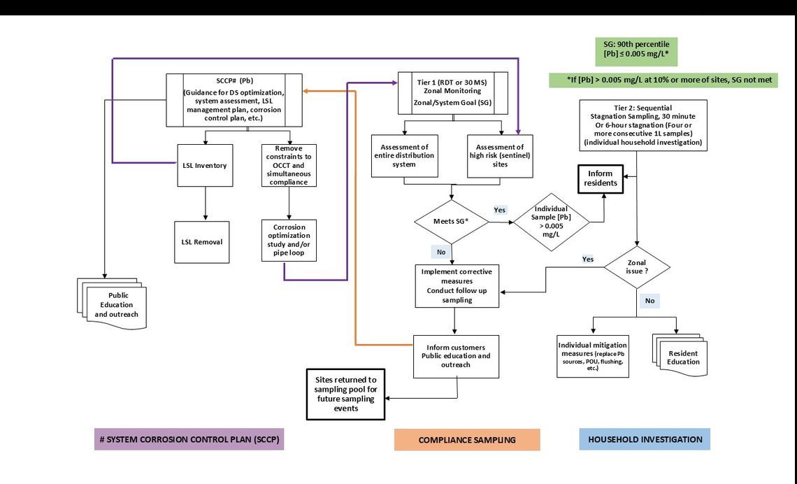
Figure E.1 - Text description
This is a flowchart outlining a framework for a residential corrosion control program. The framework describes activities and steps to undertake to achieve a holistic approach to corrosion control and corrosion control treatment. It outlines the interconnection between the various elements of the System Corrosion Control Plan such as guidance for corrosion control optimization in distribution system followed by lead service line inventory and subsequent removal of the lead service line. It also includes, in parallel, the removal of constraints to optimal corrosion control and simultaneous compliance followed by corrosion optimization study and/or pipe loop studies, which then inform the protocols for zonal monitoring of residential dwellings. The lead service line inventory informs the selection and assessment of sentinel sites, which are used in both options of the residential dwellings protocols (RDT and 30 MS). The protocol provides information on compliance sampling for the the zonal/system goal (SG) for individual household investigation sampling. The following information is presented in a box: the SG is that the 90th percentile lead concentration be equal to 0.005 mg/L which means the lead concentration is greater than 0.005 mg/L at less than 10% of sites.
Part F. Alternative monitoring protocol for non-residential and residential buildings (two-tier stagnation)
F.1 Alternative sampling protocol
The goals of this alternative sampling protocol and SG for non-residential and residential buildings, such as child care centres, schools and larger buildings, are to locate specific lead problems within the buildings and identify where and how to proceed with remedial actions. The intention is to minimize lead concentrations at the cold drinking water outlets (that is, fittings and fixtures such as faucets and fountains) used for drinking and cooking and therefore protect occupants' health from exposure to lead. The sampling protocols and SG are based on an understanding of the variations in lead concentrations observed at outlets in a non-residential building resulting from sources of lead within the plumbing and water use patterns.
Stagnation periods will be influenced by such things as the frequency of use of the outlet, whether bottled water is distributed in the building, whether the building is occupied 24 or 8 hours per day and the number of occupants. Establishing the source of the problem within a specific building becomes a critical tool in assessing which measures to take to reduce lead exposure. The locations of specific lead problems are determined by measuring lead levels at water fountains and cold drinking water outlets. When elevated concentrations of lead occur at an outlet, they can be from lead-containing material within the outlet itself (for example, faucet, bubbler, water cooler), from the plumbing upstream of the outlet or from the water entering the building. A two-tier sampling approach is used to identify the source of the elevated lead concentration.
Since elevated concentrations of lead can be found in drinking water as a result of leaching from plumbing materials, including fittings and fixtures, within a building, this protocol should be followed by responsible authorities, such as building owners or managers, school boards and employers, as part of the overall management of the health and safety of the occupants of schools, child care centres and other non-residential buildings. This protocol may also be followed by utilities that want to include non-residential or residential buildings such as schools and multi-dwelling buildings in their corrosion control monitoring programs. The extent of sampling within a building may vary depending on the goal of the sampling and the authority conducting the sampling.
In some cases, responsible authorities may want to collect Tier 1 and Tier 2 samples at the same time to eliminate the need to return to the site. In this case, authorities should be aware that the confidence in some sample results will decrease, since flushing water through one outlet may compromise the flushed samples taken from other outlets that are located in close proximity.
F.1.1 Tier 1 sampling protocol
The goal of Tier 1 sampling is to identify specific cold drinking water outlets that have elevated levels of lead following periods of stagnation. Collection of a smaller sample volume helps to pinpoint whether the source of lead is from the specific outlet and to direct the appropriate corrective measures. Tier 1 sampling should be conducted at the locations identified in the sampling plan for the non-residential/residential building. In addition, a sample that is representative of the water that is entering the building (water main sample) should be collected at each monitoring event. Water main samples should be collected from a drinking water faucet in close proximity to the service line following a period of approximately 5 minutes of flushing (longer flushing may be necessary to ensure that the sample is representative of water that has been flowing in the main). All other samples in the building should be collected using the protocol described below.
A first-draw 250 mL sample is taken at the locations identified in the sampling plan after the water has been stagnant for a minimum of 8 hours but generally not more than 24 hours. To ensure that representative samples are collected, the aerator or screen on the outlet should not be removed prior to sampling. It is recommended that samples be separated into smaller volumes (for example, 2 x 125 mL). This is a form of profile sampling that helps in the investigative phase if the analysis of the sample(s) indicates that lead is present. These smaller samples represent the water from the fitting (fountain or faucet) and a smaller section of plumbing and are more effective at identifying the source of lead at an outlet. Collecting the Tier 2 samples at the same time as Tier 1 samples has the benefit of not having to return to the location to resample in order to identify the source of lead.
The use of wide-mouth sample bottles allows the sampler to fill the bottle at a typical medium to high flow rate, which provides a more accurate result. Sample bottles with a smaller opening will be difficult to fill at a typical flow rate and provide inaccurate results with respect to potential exposure and investigative/remediation purposes.
If the lead concentration exceeds 0.005 mg/L (SG) at any of the monitoring locations, it is recommended that the following measures be undertaken:
- Notify and educate the occupants (for example, teachers, child care providers, students) of the building and other interested parties (for example, parents, occupational health and safety committees) on the sampling results and the interim measures that are being undertaken, as well as the plans for additional sampling.
- Conduct additional sampling at the outlets with lead concentrations that exceed 0.005 mg/L to determine the source of lead, as outlined in the Tier 2 protocol.
- Implement interim corrective measures immediately to reduce occupants' exposure to lead in first-draw water. These measures may include any or a combination of the following:
- cleaning debris from the screens or aerators of the outlet;
- flushing the plumbing system following periods of stagnation;
- taking the outlet out of service;
- using certified drinking water treatment devices; and
- supplying an alternative water supply.
- Where a substantial amount of debris was removed from the aerator or screen, authorities may want to retest the water from these outlets following the same protocol. If results of the retesting show lead concentrations below 0.005 mg/L, authorities should investigate whether particulate lead may be contributing significantly to elevated lead levels and whether regular cleaning of the aerator or screen should be implemented as part of the maintenance or flushing program.
F.1.2 Tier 2 sampling protocol
Tier 2 sampling is used in combination with results from Tier 1 to determine the source of the lead in the plumbing within the building. Sampling after a short period of flushing (30 seconds) will determine the concentration of lead in the water that has been stagnant in the plumbing upstream of the outlet.
At those water fountains and cold drinking water outlets with lead concentrations that exceeded 0.005 mg/L for Tier 1, a second 250 mL flushed sample is taken after the water has been stagnant for a minimum of 8 hours (but generally not more than 24 hours) and then flushed for 30 seconds. It is recommended that samples be separated into smaller volumes (for example, 2 x 125 mL). This is a form of profile sampling that helps in the investigative phase if the analysis of the sample(s) indicates that lead is present. These smaller samples represent the water from the fitting (fountain or faucet) and a smaller section of plumbing and have the added benefit of being more effective at identifying the source of lead at an outlet.
When the lead concentration in any of these second samples exceeds the 0.005 mg/L MAC, corrective measures should be undertaken immediately. Corrective measures can include interim measures—such as routine flushing of the outlet before the facility opens for a minimum of 5 minutes to obtain water from the water main, removing the outlet from service, using certified drinking water treatment devices or providing an alternative water supply—that are put in place until a permanent solution can be implemented. In addition, depending on the results of the Tier 1 and Tier 2 sampling, one or a combination of the following corrosion control measures should be initiated:
- Notify and educate the occupants of the building (for example, teachers, child care providers, students) and other interested parties (for example, parents, occupational health and safety committees) on the sampling results and the interim and long-term corrective measures that are being undertaken.
- Compare the Tier 1 and Tier 2 sampling results to determine whether the source of the lead contamination is the fitting, fixture or internal plumbing. If the results of the Tier 1 and Tier 2 sampling both indicate lead contamination, conduct additional sampling from the interior plumbing within the building to further determine the sources of lead contamination.
- Additional measures to consider:
- Flush the outlets;
- Install certified drinking water treatment devices;
- Replace the outlets, fountains or pipes;
- Remove the outlets from service;
- Replace lead brass fittings or in-line components;
- Work collaboratively with the water supplier to ensure that the water delivered to the building is not aggressive;
- Distribute an alternative water supply.
F.2 Rationale for the alternative stagnation sampling protocol
As with residential monitoring programs, each component of a sampling protocol in non-residential settings, such as the stagnation time, the volume of water collected and the SG, has important implications as to the usefulness of the data collected. Since the goals of conducting sampling in non-residential buildings are different from those in residential settings, the volume of water collected is also different.
The Tier 1 and Tier 2 sampling protocols for non-residential sites are based on the collection of a 250 mL sample volume. To evaluate the amount of lead leaching from outlets such as kitchen faucets, more than 95% of the lead can be found in the first 200–250 mL of water from the faucet (Gardels and Sorg, 1989). Lead levels in non-residential and large residential buildings have generally been found to decrease significantly following flushing of the outlet for 30 seconds. This suggests that the fountain or faucet and the connecting plumbing components can be major contributors to elevated lead concentrations at outlets in non-residential and institutional buildings (Bryant, 2004; Boyd et al., 2008a,b; McIlwain et al., 2016; Doré et al., 2018; Katner et al., 2018; Miller-Schulze et al., 2019).
The collection of a larger volume of water, such as 1 L, includes a longer line of plumbing prior to the outlet. This plumbing may contain valves, tees and soldered joints that could contribute to the lead concentration in the 1 L sample. However, it would not be possible to identify which material was releasing the lead. In addition, it is suggested that collecting such a large volume from a drinking water fountain might dilute the initial high concentrations observed in the outlet. This is not desirable, since water collected from sections of plumbing farther from the outlet typically have lower lead concentrations (U.S. EPA, 2004). Therefore, the collection of a sample volume that is smaller (250 mL) than those typically used to assess corrosion (1 L and greater) in residential dwellings of 6 units or less is considered important for sampling in non-residential buildings. A 250 mL sample volume is selected for sampling in non-residential buildings, as it represents water from the fitting (fountain or faucet) and a smaller section of plumbing and is therefore more effective at identifying the source of lead at an outlet, especially if this volume is broken down into smaller volumes (for example, 2 x 125 mL) so as to obtain a profile of the plumbing (U.S. EPA, 1994, 2006). If additional volumes of water were collected following the initial 250 mL sample (that is, 250–1 000 mL), the result from this larger volume may correspond to a lower concentration when calculated as a 1 L sample. This is due to the fact that the subsequent volumes would most likely contain lower concentrations of lead than that seen in the initial 250 mL sample and result in a dilution effect (U.S. EPA, 2004). However, studies have also shown an increase in lead concentration with increasing volume (McIlwain et al., 2016; Miller-Schulze et al., 2019).
Studies examining sources of lead at the tap have found lead solder and brass fittings to be significant sources of elevated lead concentrations following a period of stagnation (Lee et al., 1989; Singh and Mavinic, 1991; AwwaRF, 2004; U.S. EPA, 2007). Depending on the age and type of material, the concentrations of lead from brass fittings have been shown to increase significantly following stagnation periods of between 4 and 20 hours (Lytle and Schock, 2000). As a result, the water use pattern in a building is an important factor in determining lead concentrations at the tap. Since water use patterns are often intermittent in buildings such as day care centres, schools, residential and office buildings, sampling following a period of stagnation will capture this type of scenario. The most conservative standing time prior to sampling is between 8 and 18 hours, since it is most likely to result in the measurement of peak concentrations of lead. Therefore, first-flush samples should be collected following a minimum period of stagnation of 8 hours, but not greater than 24 hours, so that they are representative of the longer periods in which outlets are not used for drinking during most days of the week in a non-residential building.
F.2.1 Tier 1 sampling protocol
The Tier 1 sampling protocol has been used in non-residential and residential buildings for locating specific lead issues, determining how to proceed with remedial measures and demonstrating that remediation has been effective. Numerous studies have been published on extensive sampling programs for measuring lead concentrations at the tap, conducted in schools and other non-residential and residential buildings. These studies demonstrated that the collection of 250 mL samples following a period of stagnation of a minimum of 8 hours, but generally not more than 24 hours, is effective at identifying outlets with elevated lead concentrations (Gnaedinger, 1993; Murphy, 1993; Maas et al., 1994; Bryant, 2004; Boyd et al., 2008a,b). Using this sampling method, several studies were able to determine the source of lead within schools and develop a remediation plan (Boyd et al., 2008a,b; Deshommes et al., 2016; Doré et al., 2018).
F.2.2 Tier 2 sampling protocol
In order to help identify the source of lead at outlets that exceed the Tier 1 SG, follow-up samples are taken of the water that has been stagnant in the upstream plumbing but not in the outlet itself. The results can then be compared to assess the sources of elevated lead and to determine the appropriate corrective measures. In order to be able to compare the results, a second 250 mL sample is collected following the same period of stagnation. To obtain water that has been stagnant in the plumbing prior to the outlet, a 250 mL sample is taken after a period of stagnation of a minimum of 8 hours, but generally not more than 24 hours, followed by a 30 second flush. Water from water fountains and cold water outlets is collected after the water has been flushed for 30 seconds. This flushing should normally eliminate the water present in the outlet. If the lead concentration in the second 250 mL sample decreases below 0.005 mg/L (the SG), then it can be concluded that the water fountain, the cold drinking water outlet or the plumbing in the immediate vicinity is the source of the lead. If concentrations of lead above the 0.005 mg/L MAC are found in the Tier 2 samples, then the lead sources may include the plumbing materials that are behind the wall, a combination of both the outlet and the interior plumbing or contributions of lead from the service connection.
The results of Tier 1 and Tier 2 sampling should be interpreted in the context of the plumbing profile so that an assessment of the lead contributions can be made and the appropriate interim and long-term corrective measures can be taken. Information on other sampling that can help determine the source of lead for various plumbing configurations as well as detailed information on the interpretation of Tier 1 and Tier 2 sampling results is available in other reference material (U.S. EPA, 2018).
Part G. Additional resources on corrosion control related topics
Additional guidance on corrosion control plans, lead service line detection and removal, management of galvanized iron pipe, communications to customers and a variety of other topics can be found in the references and links listed below.
| Title of document | Topics covered | Reference |
|---|---|---|
| General information on corrosion and strategies for corrosion control | ||
| Internal Corrosion Control in Water Distribution Systems: Manual of Water Supply Practices, M58 | Fundamentals of corrosion and metal release, water quality monitoring, corrosion control techniques, monitoring tools for effectiveness of corrosion control | AWWA, 2017a |
| Water Quality in Distribution Systems: Manual of Water Supply Practices, M68 | Information on corrosion control and water quality | AWWA, 2017b |
| Lead control strategies | Sources of lead, monitoring strategies, treatment strategies | AwwaRF, 1990 |
| Post optimization lead and copper control monitoring strategies | Change in treatment or source water, home sampling, on-line monitoring | AwwaRF, 2004 |
| Optimization of phosphorus-based corrosion control chemicals using a comprehensive perspective of water quality | pH and alkalinity adjustment, phosphate dosing and optimization, water quality monitoring | Cantor, A.F. (2017). (Water Research Foundation Project #4586) Ch. 13 |
| Evaluating key factors that affect the accumulation and release of lead from galvanized pipes | Lead release from galvanized pipes, management/replacement plan framework, corrosion control information, public education, bench-scale testing information | Edwards et al., 2022 |
| Ontario Guidance Document for Preparing Corrosion Control Plans (2009) | Preparing a corrosion control plan, evaluating effectiveness of treatment measures, etc. Some information for small systems | MOE, 2009 |
| Guide de conception des installations de production d'eau potable | Design of drinking water treatment plants (French only) | MELCC, 2021a |
| Guide d'évaluation et d'intervention relatif au suivi du plomb et du cuivre dans l'eau potable | Regulation and protocols for lead in drinking water, background information, templates (French only) | MELCC, 2021b |
| Optimal Corrosion Control Treatment Evaluation Technical Recommendations for Primacy Agencies and Public Water Systems | Sources of lead and copper, water quality factors affecting lead and copper release, CCT options, monitoring of CCT, impact of treatment and source water quality changes | U.S. EPA, 2016 |
| Lead service line inventory or detection | ||
| Rapid and simple lead service line detection screening protocol using water sampling | Water sampling for lead service line detection | Schock et al., 2021 |
| Lead service line identification: A review of strategies and approaches | Review of lead service line detection approaches | Hensley et al., 2021 |
| Standard ANSI/AWWA C810-17: Replacement and flushing of lead service lines | Information on procedure for lead service line replacement and flushing following replacement | AWWA, 2017c |
| Lead service line replacement | ||
| Strategies to obtain customer acceptance of complete lead service line replacement | Strategies for customer acceptance of complete lead service line replacement | AWWA, 2005 |
| Standard ANSI/AWWA C810-17: Replacement and flushing of lead service lines | Information on procedure for lead service line replacement and flushing following replacement | AWWA, 2017b |
| Lead Service Line Replacement Collaborative | Downloadable resources on many topics related to lead service line replacement, lead service line inventory, etc. | Lead Service Line Replacment Collaborative, 2021 |
| Full Lead Service Line Replacement Guidance (Project No. 4713) | General information on sources of lead, high velocity flushing, lead service line replacements, copper solubility control. Field and case studies, toolbox for full lead service line replacements | Water Research Foundation, 2021 |
| Rehabilitation methods for lead service lines | ||
| Evaluation of Lead Service Line Lining and Coating Technologies | Information on lead service line coatings and linings; advantages, disadvantages and leaching of other chemicals; case studies | Randtke et al., 2017 (Water Research Foundation Project #4351) |
| Pipe loop/pipe rig | ||
| Development of a pipe loop protocol for lead control | Construction and operation of pipe loops, statistical evaluation recommendations, historical pipe loop studies | AwwaRF, 1994 |
| Guidance for using pipe loops to inform lead and copper corrosion control treatment decisions (Project No. 5081) | Considerations and limitation of pipe rig studies, influencing factors, design of pipe rigs, operations, data analysis, costs | Water Research Foundation, 2023 |
| Report to Health Canada on guidance for using pipe loops to inform corrosion control treatment decisions | Analysis of previous pipe loops and framework for guidance (case studies), best practices and design, statistical analysis of pipe loop data, lead solubility modelling | Centre for Water Resources Studies, 2023 |
| Schools or childcare facilities/large building *including commercial buildings | ||
| 3Ts for Reducing Lead in Drinking Water in Schools and Child Care Facilities A Training, Testing, and Taking Action Approach Revised Manual | Information on sources of lead, sampling plan development, sampling and result interpretation, remediation strategies | U.S. EPA, 2018 |
| Procédure visant à mesurer les concentrations de plomb dans l'eau potable des écoles du Québec | Lead sampling in schools (French only) | MEES 2020 |
| Gestion du plomb dans l'eau potable : un guide pour les propriétaires d'un grand bâtiment | Lead sampling in large buildings (French only) | MELCC, 2021c |
| Lead Service Line Replacement Collaborative Website | Web-based resources on schools and child care facilities | LSLR Collaborative, 2023 |
| Selecting a lead filter and cleaning aerators | ||
| Infographic: Cleaning faucet aerators | Steps to cleaning faucet aerators, remove lead and other particles | Health Canada, 2023a |
| Infographic: Finding a drinking water filter | Instructions on how to find a filter certified for lead removal | Health Canada, 2023b |
| Outreach and communications | ||
| Lead Service Line Replacement Collaborative Website | Web-based resources | LSLR Collaborative, 2023 |
Reference list for Table G.1.
- AWWA (2005). Strategies to Obtain Customer Acceptance of Complete Lead Service Line Replacement. American Water Works Association, Denver, CO. Available at: https://www.awwa.org/Portals/0/AWWA/Government/StrategiesforLSLs.pdf?ver=2013-03-29-132027-193
- AWWA (2017a). Internal Corrosion Control in Water Distribution Systems: Manual of Water Supply Practices, M58. Second edition. American Water Works Association, Denver, CO.
- AWWA (2017b). Water Quality in Distribution Systems: Manual of Water Supply Practices, M68. First edition. American Water Works Association, Denver, CO.
- AWWA (2017c). Standard ANSI/AWWA C810-17: Replacement and flushing of lead service lines. American Water Works Association, Denver, CO.
- AwwaRF (1990). Lead control strategies. AWWA Research Foundation and American Water Works Association, Denver, CO.
- AwwaRF (1994). Development of a pipe loop protocol for lead control. AWWA Research Foundation, Denver, CO.
- AwwaRF (2004). Post optimization lead and copper control monitoring strategies. AWWA Research Foundation, Denver, CO (Report 90996F).
- Cantor, A.F. (2017). Optimization of phosphorus-based corrosion control chemicals using a comprehensive perspective of water quality. Water Research Foundation and Water Environment and Reuse Foundation, Denver, Colorado. Report #4586.
- Centre for Water Resources Studies (2023). Guidance for using pipe loops to inform corrosion control treatment decisions, Dalhousie University. Report for Health Canada. Available upon request at: water-eau@hc-sc.gc.ca.
- Edwards, M., Mohsin, H., Parks, J. Masters, S.V., Arnold, R., and Rosenfeldt, B. (2022). Evaluating key factors that affect the accumulation and release of lead from galvanized pipes. Water Research Foundation, Denver, Colorado (Water Research Foundation Project No.4910).
- Health Canada (2023a). Infographic: Cleaning faucet aerators. Health Canada, Healthy Environment and Consumer Safety Branch. Available at: https://www.canada.ca/en/health-canada/services/publications/healthy-living/infographic-cleaning-faucet-aerators.html
- Health Canada (2023b). Infographic: Finding a drinking water filter certified to reduce lead. Health Canada, Healthy Environment and Consumer Safety Branch. Available at: https://www.canada.ca/en/health-canada/services/publications/healthy-living/infographic-finding-drinking-water-filter.html
- Hensley, Bosscher, V., Triantafyllidou, S., and Lytle, D.A. (2021). Lead service line identification: A review of strategies and approaches. AWWA Wat sci. Vol 3 (3): e1226. Doi.org/10.1002/aws2.1226
- Lead Service Line Replacement Collaborative (2023). Website with a variety of downloadable resources on many topics https://www.lslr-collaborative.org/
- MEES (2020). Procédure visant à mesurer les concentrations de plomb dans l'eau potable des écoles du Québec. Ministère de l'Éducation et de l'Enseignement supérieur, Direction de l'expertise et du développement des infrastructures scolaires, Direction générale des infrastructures. Québec, QC. Available at: https://www.education.gouv.qc.ca/fileadmin/site_web/documents/education/reseau/boite-outils/Procedure-concentrations-plomb.pdf
- Ministère de l'Environnement et de la Lutte contre les changements climatiques (MELCC) (2021a). Guide de conception des installations de production d'eau potable. Volumes 1 et 2. Disponible à : https://www.environnement.gouv.qc.ca/eau/potable/guide/index.htm
- Ministère de l'Environnement et de la Lutte contre les changements climatiques (MELCC) (2021b). Guide d'évaluation et d'intervention relatif au suivi du plomb et du cuivre dans l'eau potable. Québec, QC. Ministère de l'Environnement et de la Lutte contre les changements climatiques. Disponible à : https://www.environnement.gouv.qc.ca/eau/potable/plomb/guide-evaluation-intervention.htm
- Ministère de l'Environnement et de la Lutte contre les changements climatiques (MELCC) (2021c). Gestion du plomb dans l'eau potable : un guide pour les propriétaires d'un grand bâtiment. Québec, QC. Ministère de l'Environnement et de la Lutte contre les changements climatiques. Disponible à : https://www.environnement.gouv.qc.ca/eau/potable/plomb/guide-evaluation-intervention.htm
- OME (2009). Guidance document for preparing corrosion control plans for drinking water systems. Ontario Ministry of the Environment. Available at: https://ia803403.us.archive.org/35/items/guidancedocument00snsn21738/guidancedocument00snsn21738.pdf
- Schock, M. R., Lytle, D.A., James, R. R., Lal, V., & Tang, M. (2021). Rapid and simple lead service line detection screening protocol using water sampling. AWWA Water Science, e1255. https://doi.org/10.1002/aws2.1255
- U.S. EPA (2016). Optimal Corrosion Control Treatment Evaluation Technical Recommendations for Primacy Agencies and Public Water Systems. U.S. Environmental Protection Agency, Office of Water. Washington, DC. (Report No. EPA 816-B-16-003). Available at: https://www.epa.gov/sites/default/files/2019-07/documents/occtmarch2016updated.pdf
- U.S. EPA (2018). 3Ts for Reducing Lead in Drinking Water in Schools and Child Care Facilities A Training, Testing, and Taking Action Approach Revised Manual. U.S. Environmental Protection Agency, Office of Water. Washington, DC. (Report No. EPA 815-B-18-007). Available at: https://www.epa.gov/system/files/documents/2021-07/epa-3ts-guidance-document-english.pdf
- U.S. EPA (2022). Guidance for Developing and Maintaining a Service Line Inventory. U.S. Environmental Protection Agency, Office of Water. Washington, DC. (Report No. EPA 816-B-22-001). Available at: https://www.epa.gov/system/files/documents/2022-08/Inventory%20Guidance_August%202022_508%20compliant.pdf
- Water Research Foundation (2021). Full lead service line replacement guidance (Project No. 4713). Water Research Foundation. Denver, CO. Available at: https://www.waterrf.org/system/files/resource/2022-09/DRPT-4713.pdf
- Water Research Foundation (2023). Guidance for using pipe rigs to inform lead and copper corrosion Control treatment decisions (Project No. 5081). Water Research Foundation and Copper Development Association. Denver, CO. Available at: https://www.waterrf.org/research/projects/guidance-using-pipe-rigs-inform-lead-and-copper-corrosion-control-treatment
Part H. International considerations
Although various national and international organizations have established values for lead in drinking water, few have drinking water guidance or regulations for corrosion control. The U.S. EPA revised the lead action level to 0.010 mg/L (10 µg/L) in its final treatment-based Lead and Copper Rule Revisions (LCRR), published in November 2023, based on the 90th percentile of samples collected. Drinking water systems exceeding the action level must implement lead service line replacement at a minimum average annual rate of 10 percent calculated on a rolling 3-year period and initiate (or re-optimize) CCT. In addition, regulated drinking water systems were to complete initial inventories of their lead service lines by October 2024.
The U.S. EPA promulgated the final LCR Improvements (LCRI) rule on October 8, 2024. This rule requires that the vast majority of water systems replace lead service lines within 10 years and regularly update their inventories. For sites with lead service lines, water systems are required to collect and analyze the first-litre and fifth-litre of water and use the higher of the two values when determining compliance with the rule. Water systems with multiple exceedances of the lead action level are required to continue adjusting treatment, conduct additional community outreach, and provide all consumers with filters that are certified to reduce lead.
Under the final LCRI, there must be more frequent and proactive communications about lead pipes and plans for replacement.
The World Health Organization published a technical brief providing guidance on managing lead contamination in drinking-water supplies. It includes information on sampling for compliance and investigative purposes as well as interim and long-term corrective measures to undertake (WHO, 2022b).
The European Union and Australian National Health and Medical Research Council have not established guidance on corrosion control.
Footnotes
- Footnote 1
-
A residential dwelling converted to a day care facility should be sampled as a residential dwelling.
- Footnote 2
-
Based on the 90th-percentile value of the highest lead concentrations of tap samples collected during the monitoring period.