
Modelling approach to assessing risk of transmission of SARS-CoV-2 at gatherings

 Download this article as a PDF
Published by: The Public Health Agency of Canada
Issue: Volume 47-4: COVID-19: A Year Later
Date published: April 2021
ISSN: 1481-8531
Submit a manuscript
About CCDR
Browse
Volume 47-4: COVID-19: A Year Later
Modelling
Simple mathematical modelling approaches to assessing the transmission risk of SARS-CoV-2 at gatherings
David Champredon1, Aamir Fazil1, Nicholas H Ogden2
Affiliations
1 Public Health Risk Sciences Division, National Microbiology Laboratory, Public Health Agency of Canada, Guelph, ON
2 Public Health Risk Sciences Division, National Microbiology Laboratory, Public Health Agency of Canada, St.-Hyacinthe, QC and Guelph, ON
Correspondence
Suggested citation
Champredon D, Fazil A, Ogden NH. Simple mathematical modelling approaches to assessing the transmission risk of SARS-CoV-2 at gatherings. Can Commun Dis Rep 2021;47(4):184–94. https://doi.org/10.14745/ccdr.v47i04a02
Keywords: transmission risk, SARS-CoV-2, COVID-19, Canada, gatherings, mathematical modelling
Abstract
Background: Gatherings may contribute significantly to the spread of severe acute respiratory syndrome coronavirus 2 (SARS-CoV-2). For this reason, public health interventions have sought to constrain unrepeated or recurrent gatherings to curb the coronavirus disease 2019 (COVID-19) pandemic. Unfortunately, the range of different types of gatherings hinders specific guidance from setting limiting parameters (e.g. total size, number of cohorts, the extent of physical distancing).
Methods: We used a generic modelling framework, based on fundamental probability principles, to derive simple formulas to assess introduction and transmission risks associated with gatherings, as well as the potential efficiency of some testing strategies to mitigate these risks.
Results: Introduction risk can be broadly assessed with the population prevalence and the size of the gathering, while transmission risk at a gathering is mainly driven by the gathering size. For recurrent gatherings, the cohort structure does not have a significant impact on transmission between cohorts. Testing strategies can mitigate risk, but frequency of testing and test performance are factors in finding a balance between detection and false positives.
Conclusion: The generality of the modelling framework used here helps to disentangle the various factors affecting transmission risk at gatherings and may be useful for public health decision-making.
Introduction
Since the emergence of severe acute respiratory syndrome coronavirus 2 (SARS-CoV-2) in late 2019, data are available that confirm that gatherings can increase the risk of SARS-CoV-2 transmission at the population level and can even have the potential to act as super-spreading eventsFootnote 1Footnote 2Footnote 3. One of the measures that decision-makers have implemented to slow the progress of the coronavirus disease 2019 (COVID-19) epidemic has been to limit the number of people congregating together for both personal and professional reasons. Intuitively, the size of gatherings is directly related to the infection rate; hence, limiting their size would minimize COVID-19 transmission.
Beyond this simple statement, assessing the effectiveness of constraints on gatherings is difficult. Gatherings can take a multitude of different forms, from indoor toddler’s birthday parties with local guests to weddings and conference with guests from multiple communities. These different forms reflect the diversity of values of the variables that drive disease transmission during the gathering (e.g. mixing, contact rates and patterns, gathering duration, prevalence in participants at the start of the event, etc.).
Detailed transmission models tailored to specific events have been employed to capture and evaluate the complexity of transmission risk and provide insights into the role of gatherings. An in-depth literature review of modellings studies assessing the risk associated with gatherings showed that there was a consensus among models that limiting the size of gatherings helps to limit SARS-CoV-2 transmissionFootnote 3. Unfortunately, we rarely have sufficient data to parametrize such “tailored” transmission models and, if we did, generalization of their findings would be challenging.
Here, we attempt to assess the transmission risk of SARS-CoV-2 during gatherings (both unrepeated and repeated) using relatively simple and generic modelling frameworks. We focus on the general issues of risk at gatherings that can be applied to all gatherings, risk of introduction and risk of transmission during gatherings, as well as two commonly used methods of mitigating risk: testing participants and (for repeated gatherings) cohorting. Despite being limited in providing precise guidance for a particular gathering, the results presented here may still be applicable, to a varying degree, for different kinds of gathering settings and help support high-level public health decision-making. As more detailed, quantitative information on specific aspects that are expected to affect the risk of gatherings (e.g. ventilation, density of participants, levels of vocalization)Footnote 3 becomes available, the framework developed here can be better parameterized to improve more gathering-specific risk estimates.
Unrepeated gathering
Unrepeated gatherings are those that occur only once, or infrequently with a length of time between them such that they can be considered unrepeated. Examples of such gatherings could be funerals, weddings or conferences.
Introduction risk
The first determinant of risk at gatherings is the probability that at least one infectious individual is present. A general approach would be to assume that infectious individuals are picked randomly from a general population that mixes homogenously (a conservative assumption when considering transmission risk). With these assumptions, the risk of having an infectious person in a gathering is proportional to the prevalence in the general population (here termed prev). The probability at least one infectious individual is present at a gathering of size N is
pintro = 1 – (1 – prev)N
This simple expression provides several outputs of value for a decision-maker. The variable pintro is the probability that at least one infectious individual participates at a gathering of size N in a setting where the population prevalence is prev. A simple readjustment of the equation provides the largest gathering size possible for a pre-determined acceptable level of introduction risk for a given infection prevalence in the population coming to the gathering:
N = log(1 – pintro) / log (1 – prev)
Another adjustment provides the level of prevalence in the population that would exceed the predetermined acceptable level of risk of introduction for a gathering of a particular size:
prev = 1 – (1 – pintro)1/N
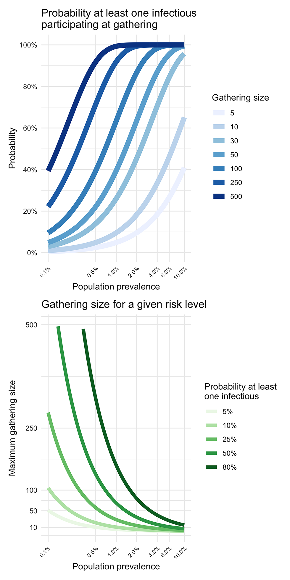
Note that while the three simple equations above cannot claim precision for a specific gathering, they can help understand how those three variables are related. The relationships between the gathering size, the prevalence in the community and the tolerance for the risk of introduction (pintro) are illustrated in Figure 1.
Figure 1: Relationships between gathering size, the prevalence in the community and the tolerance for the risk of introduction
Text description: Figure 1
The top panel displays the probability that a least one infectious individual participate at a given gathering (vertical axis). Each curve shows the probability as a function of the prevalence in the whole population, for different gathering sizes. The bottom panel shows the maximum gathering size (vertical axis) for a given prevalence of infection in the whole population (horizontal axis) and risk of introduction (coloured curves). For example, when population prevalence is 2%, the probability at least one infectious individual participates in the gathering is approximately 65%.
The assumption that the prevalence in the source population is the same as the subset attending the gathering is convenient but may not be realistic for gatherings that attract individuals from sub-populations that are either more, or less, likely to be infected.
A simple way to introduce heterogeneity is to directly change the prevalence according to the expected over or under-exposure of the participants of the gathering. The adjusted prevalence for this specific group, prevG, can be simply calculated from the baseline prevalence. If we know the relative risk RR of the group compared to the whole population, and if we know the odds ratio, OR, of infection for this group, we have
prevG = RR × prev, or prevG = (1 + (1 – prev)/(OR × prev))-1
For example, if 1) the current prevalence of SARS-CoV-2 infections in the population coming to the gathering is prev = 0.5%, 2) the gathering demographics are similar to the whole population and 3) we decide the maximum acceptable probability that an infectious individual joins this gathering is pintro = 20%, then the maximum size that the gathering should be is no more than N = 44 . However, if we consider a gathering where a group of participants are five times more likely than the general population to be infected (prevG = 5 × prev = 2.5%), then the maximum size for this gathering should not be more than nine.
Transmission risk at the gathering
Once the probability of an infected person being present at the gathering has been determined, the second question that needs to be considered is: “What is the risk that this individual transmits the pathogen to other susceptible participants?”.
If we assume homogenous mixing during a gathering of N persons at which I infectious individuals are participating, and that that any susceptible individual will contact C different persons (infectious or not) at the gathering, then the expected minimum number of transmissions that will occur during this gathering is
ntransm = (N – I) × (1 – (1 – (I/(N – 1)) ptr)C)
where C is the number of contacts during the gathering with an infectious individual and ptr is the probability of transmission given a contact with an infectious person (see Appendix for details). The variables C and ptr are context-specific and should be calibrated to the best available evidence as this becomes available from epidemiological analyses and research studies. It may be useful to work with a range of estimates that will produce upper and lower bounds for ntransm. The formula above is simple enough to be implemented in a spreadsheet and can help disentangle the role of the gathering size and measures that help reduce the transmission probability (e.g. wearing masks) or the number of contacts (e.g. physical distancing).
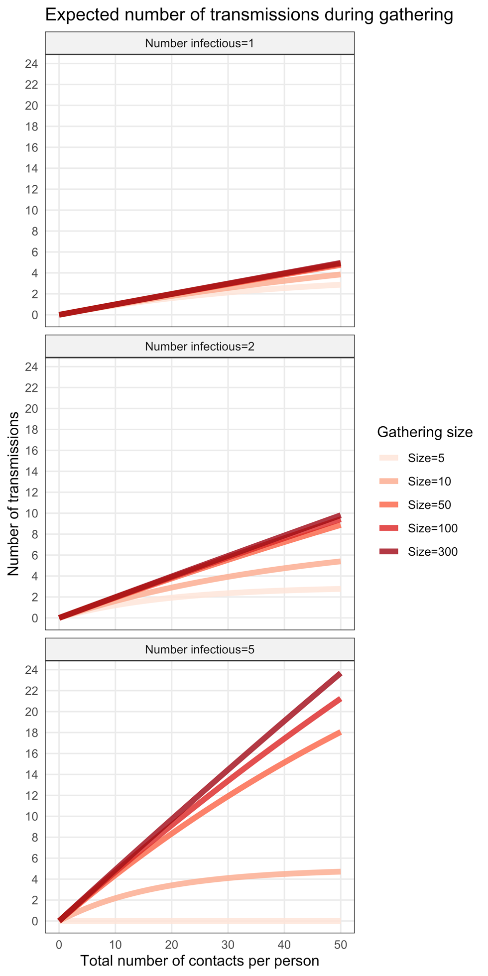
Figure 2 shows ntransm for different values of gathering sizes and infectious individuals participating. For example, we can expect that there will be about four transmissions during a 10-person gathering where two infectious individuals are participating (Figure 2, centre panel), the contact rate is on average 30 contacts per person and the probability of transmission is ptr = 10%. When only one infectious person is at a gathering (left panel), the expected number of transmissions is approximately the same for different gathering sizes. This is primarily because the probability of a susceptible person encountering an infectious person is low. The outcome was very different with five infectious people present (Figure 2, right panel). In this case, the probability that susceptible people encounter infectious people in the crowd increases and, therefore, the number of transmissions that could occur also increases.
Figure 2: Effect of gathering size and number of infected individuals on minimum number of secondary transmissions
Text description: Figure 2
The graph show the expected number of transmissions when one (top panel), two (middle panel) or five (bottom panel) infectious individuals participate in a gathering of different sizes (from 5 to 300, coloured curves). The expected number of transmissions (vertical axis) are shown as a function of the average total number of contacts per person occurring during the gathering (horizontal axis). The plots were generated using a probability of transmission given contact of ptr = 10%.
For very large gatherings, we can reasonably assume that the number of infectious participants should be approximately equal to the population prevalence, assuming the gathering is a random sample of the population.
If Cmax is the maximum number of contacts an infectious individual can make during the gathering, then A = S/(Cmax ptr) is the minimum number of infectious individuals needed to have a chance to infect all the S susceptible individuals at the gathering (all infectious would need to contact Cmax times only the susceptible individuals). Rescaling A to the gathering size leads to a = A/N. The ratio a can act as a threshold value to assess if the extreme event where every susceptible individuals could be infected at the gathering. If prev is the population prevalence, having prev ≈ a means it is possible that all susceptible individuals become infected. More generally, if prev ≈ f × a, then a fraction f of the susceptible participants is at risk of being infected during the gathering. For example, a gathering of 1,000 persons, where the maximum number of contacts for any individual is 30 and the probability that infection is transmitted when a contact takes place is 60%, has a threshold value of a = 5.5%. Hence, a population prevalence above 5.5% (i.e. if we expect more than 55 infectious participants) would be worrying for this gathering, as there is a potential to infect every susceptible participant. If the population prevalence was 2.75%, then half of the susceptible participants would be at risk of being infected (f = 0.5). The duration of the gathering also has an impact on the risk of transmission. Intuitively, the longer individuals are together, the more opportunities there are for virus-transmitting contacts to occur. The effect of time on transmissions can be modelled using survival analysis. The proportion of susceptible individuals remaining t time units after the start of the gathering (t = 0) is:
S(t) = e-λt
The infection hazard λ (assumed to be constant here) can be estimated from recorded infections at observed events (through contact tracing). This implicitly assumes that the time to infection is exponentially distributed. If N is the size of the gathering, T its duration and i the total number of transmissions that happened during this event, then a naive estimate of the infection hazard is
λest = (1/T)log (N/i)
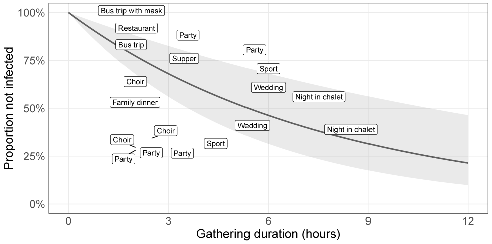
Studies reporting on contact tracing of gathering events can provide the necessary data to calculate this estimate for a given gathering. Figure 3 is an example of epidemiological data used to inform the survival model. Note that the information collected from such studies is likely conservative; gatherings that drew the attention of public health workers because of the large number of secondary cases are likely to be more reported than the ones where few or no transmission occurred. Figure 3 also shows a naive fit of the infection hazard during events (λest) to the data of Appendix Table S1. Estimates of infection hazard λest can help support decisions regarding duration limits on gatherings.
Figure 3: Infection hazard estimated from epidemiological data from social gatherings
Text description: Figure 3
Example of a naive fit to the epidemiological data presented in Appendix Table S1. Each label represents the type of gathering; its position on the graph shows its approximate duration (horizontal axis) and the proportion of participants that were not infected (vertical axis). The solid black curve is the linear regression performed on the log scale (see Appendix for details) and the grey ribbon represents the 95% CI.
Recurrent gatherings
The second category of gatherings are those that occur on a regular basis with the same participants. Examples of such gatherings are company employees, students and teaching staff at a school, and hospital staff.
Definitions and assumptions
Participants in recurrent gatherings frequently form cohorts (e.g. school classes, office staff) within which the individuals interact preferentially. Cohorting has also been considered as a mitigation measure for transmission at gatheringsFootnote 4. Furthermore, a common intervention by public health to minimize transmission at gatherings is to reduce the contact rate between cohorts as much as possibleFootnote 5.
If it is assumed there are M cohorts, G1,G2,…,GM and, for simplicity, assume that all cohorts have the same size of N individuals, then there is a total of M × N individuals that gather on a regular basis. From an epidemiological perspective, there are three main transmission pathways associated with these recurrent gatherings: introduction of infected individuals in a cohort; transmission within a cohort; and transmission between cohorts (Figure 4).
Figure 4: Transmission pathways associated with recurrent gatherings
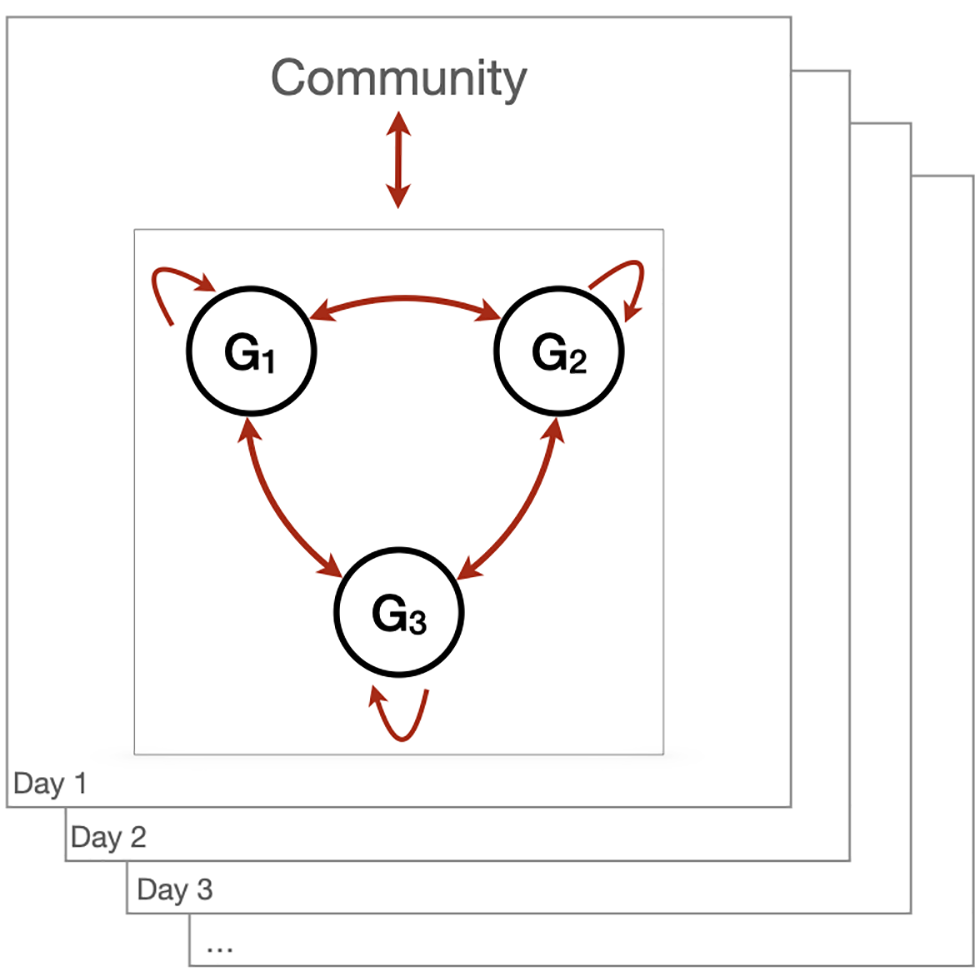
Text description: Figure 4
Individuals are assigned groups with which they will preferentially interact with. Here, this figure is an illustration with three groups/cohorts. Contact between groups G1, G2 and G3 is minimized (three cohorts are formed). Individuals gather frequently to perform their duties within this organization. Individuals live within a community where the epidemic spreads. Hence, assuming that all individuals are not infected when they start their recurrent gatherings, cohorts face an introduction risk from interactions with the community they live in, then transmission within and between groups.
Introduction risk
For recurrent gatherings, the risk of introduction can be estimated in a similar fashion to that of non-repeated gatherings, but the frequency with which the gathering occurs (t) also needs to be considered. This then estimates the introduction risk into a recurrent gathering in a community with prevalence (prev), gathering size (MN), made up of M groups of size N over the course of t days.
pintro = 1 – (1 – prev)tMN
Figure 5 illustrates that for a recurrent gathering of 100 people with different cohort sizes (20 groups, each with a cohort size of five people; 10 groups with a cohort size of 10; or five groups with a cohort size of 20), cohort size does not change the risk of introduction to the gathering as a whole. However, the risk of introduction to each individual cohort is significantly reduced by reducing the cohort size. Thus, the challenge is to develop strategies to ensure that if an infection is introduced into one of the cohorts it does not spread to the other cohorts at the gathering.
Figure 5: Introduction risk as a function of time and cohort structure
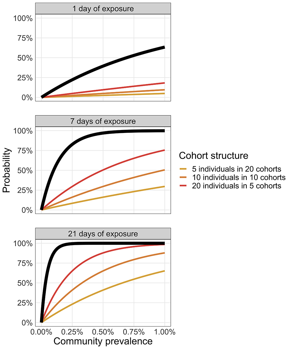
Text description: Figure 5
Each panel represents a different duration of exposure (1, 7 or 21 days). The coloured curves illustrate the introduction risk for each cohort structure and the thick black line shows the introduction probability at the organization level (i.e. considering all cohorts).
The risk of infection from the community is simply the infection prevalence in the community (assuming the gathering is representative of the population). As described above for unrepeated gatherings, if the individuals have a different prevalence, prevG, than the one found in the community, the expected prevalence can be adjusted using an estimated relative risk or an odds ratio.
Transmission within a cohort
Estimating transmission within one cohort is similar to the analysis above for unrepeated gatherings, but with a larger value for the number of contacts (C) because of the recurrent nature of the gathering.
Transmission between cohorts
The probability of transmission over the duration of infectiousness between a cohort where at least one member is infectious and any other fully susceptible cohort, is pbw. If the cohorts are completely isolated, pbw = 0, then the maximum number of secondary transmissions following the introduction of an infectious person in a cohort is limited to the cohort size, N. Recall there is a total of M×N individuals (M cohorts with N individuals each), so the overall attack rate cannot be larger than N/NM = 1/M. For example, a company that has 20 employees separated into four cohorts, each with five individuals, will have a maximum attack rate of 1/4=25% if these cohorts are kept completely isolated.
Of course, the assumption of complete isolation between cohort is rarely realistic and the probability of transmission between cohorts is greater than zero (pbw > 0). If a is the attack rate within one single cohort (0 ≤ a ≤ 1) then, assuming none of the infections is detected, the expected number of infected individuals in a cohort where the initial infectious individual was introduced is aN. Taking the approach that the seeded cohort can potentially infect any other cohort at the same time (so effectively considering only two synchronous generations of infections as well as homogeneous mixing) the overall attack rate is:
aall = a(1/M + (1 – 1/M)pbw)
When the cohorts are well isolated (pbw is very small), the overall attack rate is reduced simply by the fact of splitting the organization into M cohorts and we have aall ≈ a/M: only the cohort that experiences an introduction is affected, so the overall attack rate is diluted by the number of cohorts. At the other extreme (Figure 6, right panel), if the cohorts are poorly isolated (pbw near one) then partitioning the organization into cohorts has little effect (aall ≈ a). For low to moderate probabilities of transmission between cohorts (Figure 6, left and centre panels), increasing the number of cohorts markedly dilutes the overall attack rate (aall) when the cohort attack rate (a) is large (say, above 20%). Moreover, because of the 1/M terms, the dilution of the attack rate saturates as M increases (Figure 6).
Figure 6: Transmission risk between cohorts following a single introduction
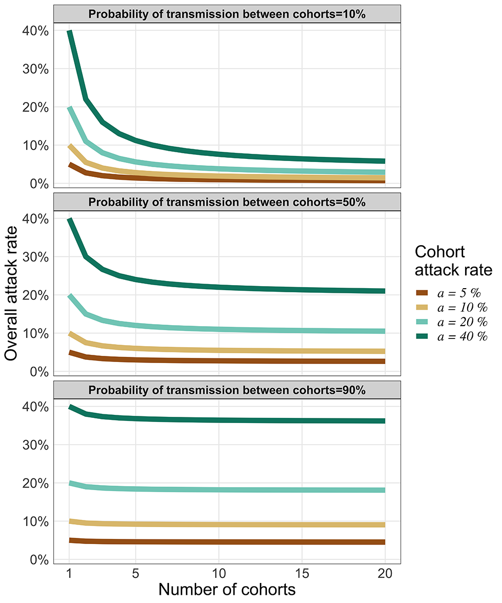
Text description: Figure 6
The vertical axis represents the overall attack rate for an organization that has separated its members in cohorts (horizontal axis). Each coloured curve represents a different cohort attack rate. Each panel illustrates how the overall attack rate (for the whole organization) varies based on three levels of isolation between cohorts (high isolation for top panel, moderate for the middle panel and low isolation for the bottom panel)
Mitigation using testing
Reducing the risk of infections at a gathering can be achieved by reducing the chances of contacts, by reducing the probability of transmission given a contact or both. Physical distancing, for example keeping at least two meters between participants, can reduce the probability of contact. Hand washing, surfaces sanitation and the proper use of masks have all been shown to reduce the probability of transmission.
A third strategy to limit the transmission risk is testing participants before (for unrepeated gatherings) or during (for recurrent gatherings) the gathering(s).
Pre-gathering testing
There are two types of tests currently available to diagnose a SARS-CoV-2 infection: a polymerase chain reaction (PCR)-based assay performed in well-equipped laboratories and a rapid, often point-of-care, test, which is antigen-based (e.g. the PanBioTM COVID-19 Ag Rapid Test, Abbott Point of Care Inc.). The former is considered the gold standard but usually suffers from a long turnaround time, which can make its use impractical shortly before a gathering. The latter could be deployed just before a gathering, to filter out infected participants, but it generally suffers from a poor sensitivity when used on asymptomatic individualsFootnote 6. Testing of saliva samples, which are less invasive to obtain than the nasopharyngeal swabs used currently for PCR-based assays, would increase the possibility of repeat testingFootnote 7. The application of routine repeat testing to enhance detection of transmission at gatherings and workplaces is an ongoing field of researchFootnote 8.
Assuming that all the logistical hurdles associated with performing tests shortly before a gathering can be overcome, the testing of participants at a gathering could help reduce the transmission risk.
Accounting for transmission risk must take into consideration different durations when infections might be detectable. In a scenario in which viral shedding lasts for D days after the day of infection, the incubation period is B days, the minimum detectable viral concentration is reached after δ days and the asymptomatic fraction of infection in the population is a.
We assumed an infected individual would not attend a gathering once symptoms started. Thus, for symptomatic individuals, the window to identify them is (B – δ) days over a total period of B days. In contrast, for infected but asymptomatic individuals, the window to identify them is longer, D – δ days over a total of D days (see Figure 7). Symptomatic individuals were assumed to attend a gathering only during their pre-symptomatic infectious period.
Figure 7: Window of viral infection detectability vary between symptomatic and asymptomatic individuals
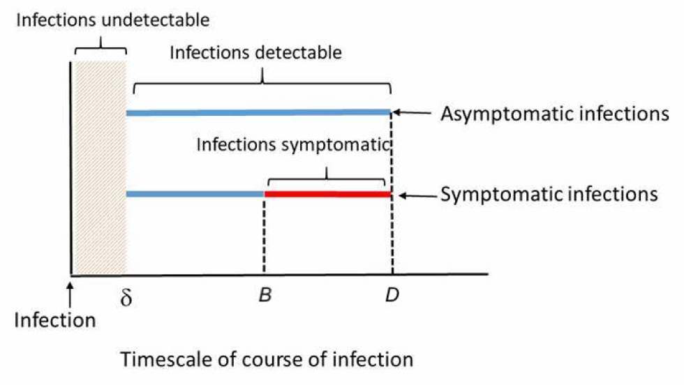
Text description: Figure 7
Blue lines indicate a detectable infection and the red line indicates viral infection not detectable (since it is assumed that an infected individual would not attend a gathering when symptoms are present). The incubation period is represented by B and the infectious period by D.
Hence, the probability that an infectious individual would be tested while the viral load is in the detectable window is
pdetectable = (1 – α)((B – δ)/B) + α((D – δ)/D)
For example, taking parameters typical of a SARS-CoV-2 infection we have B = 5 days, D = 20 daysFootnote 9, a = 30% and δ = 1 day we have pdetectable = 84.5%. In other words, about one out of six infectious participants will not be within the window of viral infection detectability.
Mitigating introduction and transmission risk with testing
There are numerous ways, most of them setting-specific, to reduce the risk of introduction and onwards transmission in recurrent gatherings. In this section, we focus on mitigating the transmission risk using periodic testing.
To reduce the risk of introduction and onward transmission to other cohorts (and to the community), we can test periodically, say every τ days, all individuals in all cohorts. It is assumed that the duration of infectiousness is fixed at D days and that a test is available that can detect infection with specificity sp and sensitivity se. Note that the detection can occur at any testing point during the infectiousness period, not just at the start (Figure 8).
Figure 8: Periodic testing in relation to the infectious period
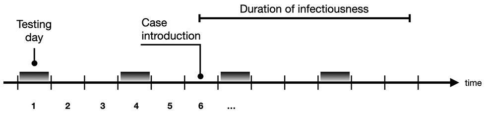
Text description: Figure 8
Illustration of periodic testing in relation with the infectious period. In this example, tests are performed every three days (τ = 3).
The probability of assessing the absence of a disease in a group using multiple rounds of testing has been extensively covered in veterinary epidemiology and is often referred to as “freedom from disease”Footnote 10. Given a sensitivity se for a test performed on n individuals every τ days over T days, the probability of detecting an infection is
pdetect = 1 – (1 – prev × se)nT/τ
where prev is the prevalence in the group testedFootnote 11. Note that pdetect may overestimate the actual probability if the periodical tests are correlated with one another (for example when testing the same individuals).
To maximize the probability of detection, the tests could be done daily. This is becoming increasingly possible thanks to point-of-care antigen-based tests. However, if the test has suboptimal specificity, false positives could impose unnecessary constraints (such as closure, isolation of personnel) on the organization (school, business, hospital). The probability that, when testing n uninfected individuals, at least one test returns a false positive result during this period is (see Appendix for details).
pfalse alarm = 1 – spnT/τ
Figure 9 illustrates the balancing act between maximizing the probability of detection (pdetect) and minimizing the nuisance of false alarms (pfalse alarm) when choosing the testing frequency (τ) and the sample size to test within the groups (n).
Figure 9: Trade-off between the probability of detecting an infectious case and a false positive
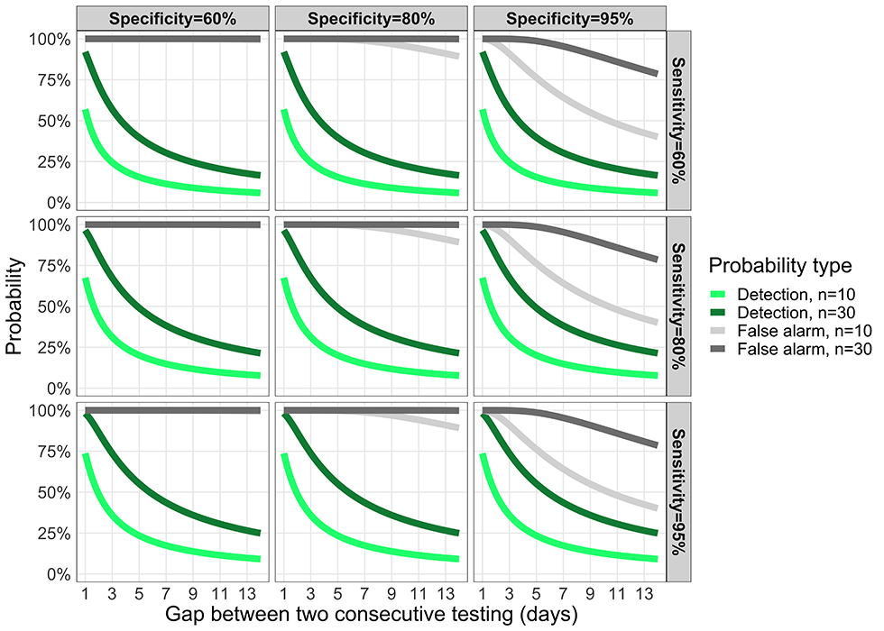
Text description: Figure 9
Trade-off between the probability to detect an infectious case and the probability of a false positive as a function of the testing frequency (horizontal axis; 1 means testing every day, 7 means every week). The green curves represent the probability to detect the first individual during her/his infectious period, here set at D =14 days when testing n individuals in the organization. The grey curves represent the probability to have a false positive for n persons tested. Each panel has different values of test specificity and sensitivity (top left panel is the least accurate, bottom right panel is the most accurate).
Time from infection to discovery
Given a testing frequency and a test accuracy, what is the expected duration between the introduction of an infectious case and its detection? If we assume an individual can be infected at any time between two consecutive tests, we can show that the time from infection to discovery is bounded by the following quantity:
tdiscovery ≤ min(D,τ (1/se – 1/2))
The effect of test sensitivity and test frequency on the time-to-discovery (tdiscovery) is illustrated in Figure 10. For a high testing frequency (e.g. less than every three days) we see that the test sensitivity does not have a large impact on the speed of detection (Personal communication, Dr. Troy Day, Queen’s University, Kingston, ON)Footnote 12.Figure 10: Testing frequency determines time from introduction of an infection to its detection
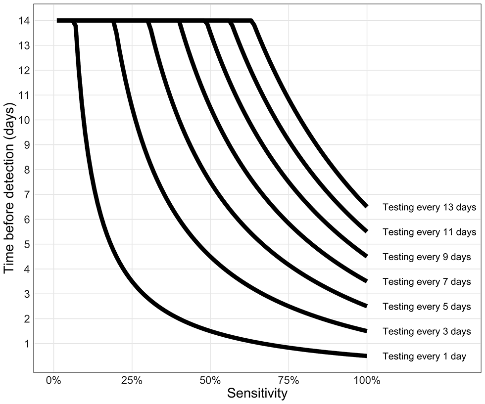
Text description: Figure 10
This graph shows the effect of test sensitivity and the frequency of testing on the time interval between infection and detection.
A natural comparison unit for tdiscovery is the generation interval. The generation interval is the interval between the time when an individual is infected by an infector and the time when this infector was infected. To slow an epidemic, tdiscovery should be much smaller than the generation interval, to prevent opportunities of secondary transmissions.
Discussion
In this study we have developed a simplistic and generic model framework to assess the risk of SARS-CoV-2 transmission at gatherings. In so doing, we have highlighted some key features of risk at gatherings, and two methods that can be used to mitigate risks.
The first determinant of risk at gatherings is the probability that at least one infectious individual is present (“introduction risk”). This risk can be broadly assessed with the population prevalence and the size of the gathering. Super-spreading events often occur during gatheringsFootnote 1Footnote 2Footnote 3. Intuitively, limiting the size of gatherings reduces the likelihood of such super-spreading events. Several modelling studies have associated smaller gathering sizes with lower reproduction numbersFootnote 13Footnote 14.
The second determinant is the risk of onwards transmission at the gathering, which is mainly driven by the gathering size and by how many contacts were present at the gathering. Our simple modelling framework highlighted the saturating effect of the contact rate (Figure 2), that is, the transmission risk is markedly reduced only when the contact rate is sufficiently low.
For recurrent gatherings, cohorting generally reduces risk of transmission, and those gatherings with a small number of well-isolated cohorts are less risky than those with a large number of poorly isolated cohorts. How the cohorts are structured (few with many individuals versus many with few individuals) does not have a significant impact on transmission between cohorts. A smaller cohort will, however, reduce the maximum number of people that can be infected if an infection is introduced into the gathering and the cohorts are well isolated.
The probability of an infectious person arriving at the gathering is a function of the prevalence of COVID-19 within the community. Testing is a mitigation option that could be employed as the attendees arrive at the gathering; however, we demonstrated that deciding on the frequency of testing with an imperfect test may be a balancing act between the efficiency of detection and the nuisance of false positives.
The findings presented here are broadly in accordance with models that are more complexFootnote 3 as well as similar simple approachesFootnote 15. The limitations of the simple approach to quantify “gathering risk” is illustrated by Figure 3 where many factors (e.g. indoors/outdoors, age of participants) can affect the transmission risk for a given gathering type. To some extent, as knowledge increases from epidemiological investigations and prospective studies, more precise values for variables such as transmission probabilities can be used to improve the parametrization of the model. However, the high-level approach here cannot replace more in-depth and detailed modelling analysis, which can take into account the multiple factors affecting transmission risk including quantifying and representing contact patterns between age groups, effects of ventilation, masks or physical distancing.
There is still a lot of uncertainty regarding the quantitative contribution from the myriad of factors that influence transmission of SARS-CoV-2 in gatherings. As evidence accumulates, we will be in a better position to inform the variables that encompass multiple underlying factors; for example, the probability of transmission presented here should be informed by indoors/outdoors settings, distance between individuals, mask usage, etc. Listing exhaustively those factors and assessing their importance regarding the transmission risk of SARS-CoV-2 at gatherings should be the focus of future studies.
Conclusion
Introduction risk can be broadly assessed with the prevalence of COVID-19 within the population and the size of the gathering, while transmission risk at a gathering is mainly driven by the gathering size. For recurrent gatherings, the cohort structure does not have a significant impact on transmission between cohorts. Testing strategies can mitigate risk, but frequency of testing and test performance are factors in finding a balance between detection and false positives.
The simple modelling framework presented here brings clarity in the interactions between the variables at play (number of participants, contact rates, etc.) in assessing the epidemiological risk. It can be used to provide a first-step assessment of risk of a gathering, and the possibility of mitigating risk. The generality of the modelling framework used here helps to disentangle these various factors affecting transmission risk at gatherings and may be useful for public health decision-making.
Authors’ statement
- DC — Conception, formal analysis, writing–original draft, writing–review and editing
- AF — Conception, drafting analysis, revising of writing, critical review
- NHO — Conception, revising of writing, critical review
Competing interests
None.
Acknowledgements
None.
Funding
None.
References
- Footnote 1
-
Adam DW, Wu P, Wong JY, Lau EH, Tsang TK, Cauchemez S, Leung GM, Lowling BJ. Clustering and superspreading potential of severe acute respiratory syndrome coronavirus 2 (SARS-CoV-2) infections in Hong Kong. Nat Med 2020;26(11):1714-9. https://doi.org/10.1038/s41591-020-1092-0
- Footnote 2
-
Kyriakopoulos AM, Papaefthymiou A, Georgilas N, Doulberis M, Kountouras J. The Potential Role of Super Spread Events in SARS-COV-2 Pandemic; a Narrative Review. Arch Acad Emerg Med. 2020;8(1):e74.
- Footnote 3
-
Public Health Agency of Canada. National Collaborating Center for Methods and Tools Evidence Brief of Size of Gatherings and Characteristics of High Risk Transmission Event; 2020. https://www.nccmt.ca/covid-19/covid-19-evidence-reviews/194
- Footnote 4
-
Tupper P, Boury H, Yerlanov M, Colijn C. Event-specific interventions to minimize COVID-19 transmission. Proc Natl Acad Sci USA 2020;117(50):32038-45. https://doi.org/10.1073/pnas.2019324117
- Footnote 5
-
Province of Alberta. Stronger public health measures: Gathering restrictions. Government of Alberta; 2020. https://www.alberta.ca/enhanced-public-health-measures.aspx
- Footnote 6
-
Corman VM, Haage VC, Bleicker T, Schmidt ML, Muhlemann B, Zuchowski M, Lei WKJ, Tscheak P, Moncke-Buchner E, Mller MA, Krumbholz A, Brexler JF, Drosten C. Comparison of seven commercial SARS-CoV-2 rapid Point-of-Care Antigen tests. medRxiv. 2020.11.12.20230292. (Epub ahead of print). https://doi.org/10.1101/2020.11.12.20230292
- Footnote 7
-
Yee R, Truong T, Pannaraj PS, Eubanks N, Gai E, Jumarang J, Turner L, Peralta A, Lee Y, Bard JF. Saliva is a Promising Alternative Specimen for the Detection of SARS-CoV-2 in Children and Adults. medRxiv. 2020.10.25.20219055. (Epub ahead of print). https://doi.org/10.1101/2020.10.25.20219055
- Footnote 8
-
Zhang K, Shoukat A, Crystal W, Langley JM, Galvani AP, Moghadas SM. Routine saliva testing for the identification of silent COVID-19 infections in healthcare workers. medRxiv. 2020.11.27.20240044. (Epub ahead of print). https://doi.org/10.1101/2020.11.27.20240044
- Footnote 9
-
He X, Lau EH, Wu P, Deng X, Wang J, Hao X, Lau YC, Wong JY, Guan Y, Tan X, Mo X, Chen Y, Liao B, Chen W, Hu F, Zhang Q, Zhong M, Wu Y, Zhao L, Zhang F, Cowling BJ, Li F, Leung GM. Temporal dynamics in viral shedding and transmissibility of COVID-19. Nat Med 2020;26(5):672-5. https://doi.org/10.1038/s41591-020-0869-5
- Footnote 10
-
Ziller M, Selhorst T, Teuffert J, Kramer M, Schlüter H. Analysis of sampling strategies to substantiate freedom from disease in large areas. Prev Vet Med 2002;52(3-4):333-43. https://doi.org/10.1016/S0167-5877(01)00245-8
- Footnote 11
-
Cannon RM. Demonstrating disease freedom-combining confidence levels. Prev Vet Med 2002;52(3-4):227-49. https://doi.org/10.1016/S0167-5877(01)00262-8
- Footnote 12
-
Larremore DB, Wilder B, Lester E, Shehata S, Burke JM, Hay JA, Tambe M, Mina MJ, Parker R. Test sensitivity is secondary to frequency and turnaround time for COVID-19 surveillance. medRxiv. 2020.06.22.20136309. (Epub ahead of print). https://doi.org/10.1101/2020.06.22.20136309
- Footnote 13
-
Saidan MN, Shbool, MA, Arabeyyat OS, Al-Shihabi ST, Al Abdallat Y, Barghash MA, Saidan H. Estimation of the probable outbreak size of novel coronavirus (COVID-19) in social gathering events and industrial activities. Int J Infect Dis 2020;98:321-7. https://doi.org/10.1016/j.ijid.2020.06.105
- Footnote 14
-
Scire J, Nadeau S, Vaughan T, Brupbacher G, Fuchs S, Sommer J, Koch KN, Misteli R, Mundorff L, Götz T, Eichenberger T, Quinto C, Savic M, Meienberg A, Burkard T, Mayr M, Meier CA, Widmer A, Kuehl R, Egli A, Hirsch HH, Bassetti S, Nickel CH, Rentsch KS, Kübler W, Bingisser R, Battegay M, Tschudin-Sutter S, Stadler T. Reproductive number of the COVID-19 epidemic in Switzerland with a focus on the Cantons of Basel-Stadt and Basel-Landschaft. Swiss Med Wkly 2020;150:w20271. https://doi.org/10.4414/smw.2020.20271
- Footnote 15
-
Tupper P, Colijn C. COVID-19's unfortunate events in schools: mitigating classroom clusters in the context of variable transmission. medRxiv 2020.10.20.20216267. (Epub ahead of print). https://doi.org.10.1101/2020.10.20.20216267
Appendix
Probability of introduction in recurrent gatherings
The probability of having at least one individual from one group Gi being infected on any given day is day is
p1 = 1 – (1 – prev)N
For this group, the probability that no introduction occurs during t consecutive days is (1 – p1)t. The probability that at least one of the M groups has an introduction is 1 – ((1 – p1)t)M, substituting p1 we have
pintro (t) = 1 – (1 – prev)tMN.
Transmission risk in a gathering
Assuming homogeneous mixing at a gathering, the probability that one susceptible individual contacts an infectious one is
P(one susceptible contacts one infectious) = I/(N–1)
If the susceptible individual has C contacts during the gathering, the probability that at least one of these contacts is with an infectious individual is
pC = 1 – (1 – I/(N–1))C
Transmission between cohorts
The expected number of secondary infections following a single introduction is
E(Aall) = aN + aN (M – 1)pbw
The first term (aN) represents the number of infections generated from the cohort first infected because of a single introduction. The second term represents the onward infections to the remaining M – 1 cohorts. To have the overall attack rate we need to normalize by the group size, hence dividing by MN gives
aall = a(1/M + (1 – 1/M)pbw)
Nuisance probability
The probability that all tests return negative from an uninfected individual tested every τ days over T days is spT/τ. Similarly, if we now consider n uninfected persons, all tested every τ days, the probability that all of these tests return negative is spT/τ. Hence, the probability that at least one test returns positive (a false alarm) during this period is 1 – spnT/τ.
Time from infection to discovery
Let Lo be the length of time between the introduction and the next test and assume it is uniformly distributed between 0 and τ. The number of false positive tests until detection, X, is assumed to be geometrically distributed and we have P(X = k) = (1 – se)k se, where se is the test sensitivity. The theoretical length of time before detection is then defined as
L = L0 + τX
The expectation for L is simply E(L) = τ/2 + τ(1 – se)/se where the first term comes from the assumption that L0 is uniformly distributed and the second term from the geometric distribution for X. The duration of infectiousness D is finite so the time to infection discovery L is naturally bounded by D. Applying Jensen's inequality for the concave function f(x) = min(x,D), we have:
E(min(L,D)) ≤ min(D,τ((1/se) – (1/2)))
Table of data source
| Event | Country | Gathering size | Rlo | Rhi | Duration (h)Table S1 footnote b | Source |
|---|---|---|---|---|---|---|
| Choir | United States | 61 | 30 | 50 | 2.5 | Tupper et al., 2020 |
| Restaurant | China | 83 | 10 | 10 | 2 | Tupper et al., 2020 |
| Party | Japan | 90 | 5 | 10 | 4 | Tupper et al., 2020 |
| Family dinner | China | 7 | 3 | 3 | 2 | Tupper et al., 2020 |
| Night in chalet | France | 10 | 4 | 9 | 8 | Tupper et al., 2020 |
| Night in chalet | France | 5 | 1 | 3 | 8 | Tupper et al., 2020 |
| Bus trip | China | 39 | 5 | 5 | 2 | Tupper et al., 2020 |
| Bus trip with mask | China | 14 | 0 | 0 | 0.83 | Tupper et al., 2020 |
| Supper | Canada | 120 | 24 | N/A | 3 | CTV news |
| Sport | Canada | 72 | 24 | N/A | 6 | The National Post |
| Sport | Canada | 21 | 15 | N/A | 4 | Montreal Gazette |
| Choir | France | 27 | 19 | N/A | 2 | Charlotte, 2020 |
| Wedding | Germany | 111 | 61 | N/A | 6 | Gelderlander |
| Wedding | Australia | 120 | 42 | N/A | 6 | The Daily Mail |
| Party | United States | 10 | 7 | N/A | 3 | Ghinai et al., 2020 |
| Party | Portugal | 100 | 16 | N/A | 6 | The Portugal Resident |
| Party | United States | 25 | 18 | N/A | 2 | WFAA |
| Party | United States | 25 | 18 | N/A | 2 | The Gainesville Sun |
| Choir | Netherlands | 80 | 32 | N/A | 2 | Omroepgelderland |
