Original quantitative research – Using classification and regression trees to model missingness in youth BMI, height and body mass data

Abstract

Introduction: Research suggests that there is often a high degree of missingness in youth body mass index (BMI) data derived from self-reported measures, which may have a large effect on research findings. The first step in handling missing data is to examine the levels and patterns of missingness. However, previous studies examining youth BMI missingness used logistic regression, which is limited in its ability to discern subgroups or identify a hierarchy of importance for variables, aspects that may go a long way in helping understand missing data patterns.

Methods: This study used sex-stratified classification and regression tree (CART) models to examine missingness in height, body mass and BMI data among 74 501 youth participating in the 2018/19 COMPASS study (a prospective cohort study examining health behaviours among Canadian youth), where 31% of BMI data were missing. Diet, movement, academic, mental health and substance use variables were examined for associations with missingness in height, body mass and BMI.

Results: CART models indicated that the combination of being younger, having a self-perception of being overweight, being less physically active and having poorer mental health yielded female and male subgroups highly likely to be missing BMI values. Survey respondents who did not perceive themselves as overweight and who were older were unlikely to be missing BMI values.

Conclusion: The subgroups identified by the CART models indicate that a sample that deletes cases with missing BMI would be biased towards physically, emotionally and mentally healthier youth. Given the ability of CART models to identify these subgroups and a hierarchy of variable importance, they are an invaluable tool for examining missing data patterns and appropriate handling of missing data.

Keywords: missing data, decision trees, overweight, obesity, adolescents

Introduction

Missing data in overweight and obesity literature

As one of the strongest predictors of chronic diseases,^{Footnote 1} overweight and obesity (OWOB) remains one of the top health concerns globally. Many studies that examine OWOB use body mass index (BMI) derived from self-reported measures of height and body mass to provide a proxy measure of body adiposity. Self-reported measures are usually less accurate than direct anthropomorphic measurements—individuals tend to underreport their body mass and overreport their height^{Footnote 2Footnote 3Footnote 4Footnote 5}—but self-reporting is generally more feasible (logistically and financially) than other approaches to population surveillance,^{Footnote 3Footnote 4Footnote 5} and these measures are useful in the appropriate context where the limitations of the data are understood.

A less-discussed methodological issue associated with self-reported height and body mass is nonresponse (i.e. missing data). Among youth, who are a primary target in the OWOB prevention literature, large proportions (sometimes over 50%) of self-reported height and body mass data tend to be missing.^{Footnote 6Footnote 7} If data are missing completely at random (MCAR), the probability of missingness depends neither on the hypothetical true value of the missing variable (i.e. what the value would be if it was reported), nor on any observed covariates. But if data are missing at random (MAR) or not missing at random (NMAR), the probability of missingness depends on observed covariates (for missing at random) and/or the hypothetical true value of the missing variable (for not missing at random). Deleting these missing cases (a method called complete case analysis) is a problematic approach, particularly for the last two mechanisms, as it leads to statistical bias.^{Footnote 8} For example, if data are missing at random because younger youth are more likely to neglect reporting their weight, the sample is biased towards older individuals (and then, logically, heavier ones, given child growth patterns).

This introduction of statistical bias as a result of deleting cases has also been proven through numerous simulation studies; it is particularly prominent when there is a large proportion of non-random missingness.^{Footnote 8Footnote 9} Despite this, complete case analysis remains the most common approach in epidemiological literature.^{Footnote 10Footnote 11} The high degree of missingness in youth self-reported height and body mass data raises concerns about how methods take into account missing data and how mishandling of missing data affects research findings as well as concomitant policy and programming recommendations.

Statistical approaches are often required to deal with missing data; while researchers should follow best practices in survey design, in many cases there may be little they can do to improve reporting patterns.^{Footnote 12Footnote 13} Although sophisticated statistical approaches to handling large proportions of non-random missingness are available, they generally require more time and expertise, which may be a barrier to their overall use. That being said, an important initial step towards selecting a reasonable and practical method for handling missing data is understanding the extent and patterns of missingness in a dataset. This is important to understand potential sources of nonreporting bias, but may also be a necessary step to identify inputs for certain missing data approaches (e.g. multiple imputation). Identifying various sources of missingness is especially important in large datasets with many variables, as methods for handling missingness can become exponentially complicated. Moreover, given that missingness is generally unique to studies, there is no clear framework for the process for identifying sources or mechanisms of missingness.

Regression approaches

Research examining BMI or body mass missingness has used regression approaches^{Footnote 6Footnote 7Footnote 14} where the outcome of a logistic regression is missing versus not missing, and other variables are examined for their potential association with the likelihood of missingness. However, regression approaches may not be ideal in this situation because missingness models may be more complex than a simplistic regression approach allows. Moreover, the process for variable selection in regression models can be ambiguous. When building a regression model, an initial step to selecting variables might be to review the literature for similar analyses, but the literature in the context of examining BMI missingness is scarce.

Bivariate comparisons are also sometimes used to decide on regression inputs; however, for large datasets with substantial missingness, this may not be useful for elimination purposes as many bivariate associations may be statistically significant. Common model selection procedures, such as the Akaike information criterion (AIC) or the Bayesian information criterion (BIC), can be used to select variables, but these procedures can be challenging in practice: we previously examined BMI, height and body mass missingness using model selection procedures for generalized linear mixed models,^{Footnote 15} but this required many additional modelling decisions and a customized algorithm suitable for pseudo-likelihood methods.^{Footnote 16}

Lastly, where variable selection processes yield a large number of relevant variables, the decision process for what to exclude in order to produce a parsimonious model may not be clear. In such cases, identifying a hierarchy of the importance of variables would be beneficial: it may help with parsimony and clearer interpretation, and it may be a necessary step to employ certain missing data approaches like multiple imputation. Although our previous study added to the literature on missingness in youth BMI, we were unable to identify which variables were most important or identify which combinations of factors were most likely to lead to nonreporting.^{Footnote 15} The limitations associated with a regression approach to examining missing data may be addressed by using a different methodological approach.

Decision trees

Decision trees are a type of machine-learning approach that has been leveraged in applied research, including in public health.^{Footnote 17Footnote 18} Decision trees are useful for analyzing primary data and for examining missing data; they can be a solution to some of the variable selection problems described above. Decision trees recursively split the data by predictor variables and can handle large datasets with multiple predictors measured on different scales with relative ease. Once pruned, decision trees present a parsed selection of predictor variables in a hierarchical format, allowing some inference on variable importance. Moreover, decision trees allow important and highly specific subgroups to be identified beyond what would be feasible using interaction terms in a regression model.

In addition, unlike regression, the entire decision tree model can be easily visualized, which may help interpretation. In 2015, Tierney et al.^{Footnote 19} published work demonstrating the utility of using decision trees to examine missing data, but to our knowledge no published studies have leveraged this approach.

The purpose of this study is (1) to add to the limited literature on missing data in youth self-reported height and body mass; (2) to identify potential areas of bias stemming from nonreporting in the youth OWOB domain; and (3) to demonstrate the use of decision trees to model missing data, which builds on the work of Tierney et al.,^{Footnote 19} who first identified the utility of this approach.

Methods

Sample

This study uses a large cross-sectional dataset from the 2018/19 wave of the COMPASS (Cannabis, Obesity, Mental health, Physical activity, Alcohol, Smoking, Sedentary behaviour) study, a prospective cohort study that collects data on a variety of different health behaviours among youth. The 2018/19 COMPASS wave collected data from 74 501 youth, representing an 84.3% participation rate. COMPASS uses an active-information, passive-consent protocol that yields high participation rates, and non-participation is usually due to absence from school on the data collection day or being in a scheduled spare during the data collection time.

Variables

This study focusses on missingness in BMI values as well as missingness in the height and body mass variables used to derive BMI. Binary indicators of missingness (i.e. missing vs. not missing) were created for each of these variables. Body mass was recorded based on responses to the question asked of students, “How much do you weigh without your shoes on? (Please write your answer in pounds OR in kilograms, and then fill in the appropriate numbers for your weight.)” Height was similarly recorded in response to the question, “How tall are you without your shoes on? (Please write your height in feet and inches OR in centimetres, and then fill in the appropriate numbers for your height).” BMI is derived by dividing body mass (kg) by height squared (m²).

A benefit of decision tree approaches is the feasibility of including many variables. In this study, we included a variety of diet, movement, academic, mental health and substance use variables. Diet-related variables included number of servings of fruits and vegetables, grain products, meat and alternatives, and milk and alternatives as well as number of days per week when breakfast, energy drinks and fast foods were consumed. Movement-related variables included moderate-to-vigorous physical activity, sports participation (inside or outside of school), strength training, physically active peers, screen time sedentary behaviour (STSB) and sleep.

Academic-related variables included English grade (or French grade, for French language schools), Math grade and truancy. Mental health variables included clinically relevant symptoms of depression (CESD-R-10 scale^{Footnote 20}), anxiety (GAD-7 scale^{Footnote 21}), socioemotional skills (DERS scale^{Footnote 22}), self-reported well-being (Flourishing scale^{Footnote 23}), self-concept (Self Description Questionnaire II short form^{Footnote 24}), self-rated mental health and reported status as a bullying victim or perpetrator. Substance use–related variables included binge drinking, smoking, e-cigarette use, cannabis use and use of alcohol mixed with energy drinks. Although all these variables were input into analyses, only a subset of variables appeared in the final models.

Outliers

In some cases, missingness was imposed onto the data. We used the 1.5 × interquartile range (IQR) method to identify statistical outliers, and these cut-offs were considered alongside biological plausibility in order to determine how to handle these cases. We marked as missing weights less than 45 lbs (20 kg) or greater than 390 lbs (177 kg) and height less than 4' (1.22 m) or greater than 6'11″ (2.11 m). Sleep and STSB were two variables that had a number of unfeasible outliers in the dataset. Youth who reported regularly sleeping less than 4 hours a night or having a collective STSB greater than 16.25 hours per day were marked as missing. Notably, missingness was only imposed for that particular variable; for example, those who reported less than 4 hours of sleep had their sleep value marked as missing, but all other reported variables remained the same.

Analysis

We used classification and regression trees (CART) as the approach for this study where the outcome was binary (i.e. missing vs. not missing). All models were stratified by self-reported sex (female, male). Consistent with decision tree approaches,^{Footnote 25} the data were split into training and testing datasets, which contained 80% and 20% of the data, respectively. The training dataset was used to fit the tree, while the testing dataset was used to assess the prediction accuracy of the training tree.

We used cost complexity pruning alongside the one standard error (1-SE) rule^{Footnote 25} to help correct for overfitting and yield a more parsimonious final tree. Decision tree analyses were conducted in R (R Foundation for Statistical Computing, Vienna, AT) using the rpart package, and final pruned trees were visualized using the rattle package. A pre-pruning restriction was set so that final nodes had to contain a minimum number of individuals. The minimum number of individuals in a school for each stratified sample was used to determine these cut-offs; this was 14 for females and 16 for males. Models included individuals with missing covariate data, as CART conveniently handles this by surrogate splitting; if a covariate value is missing, an observed variable with the most similar predictive capacity is used instead.

Results

Descriptive statistics

Table 1 shows stratified descriptive statistics for any variable that appeared in at least one of the CART models. Of the whole sample (n = 74 501), 31% were missing BMI values. Height missingness was slightly more prevalent among males (19%) than among females (15%), whereas body mass missingness was slightly more prevalent among females (22%) than among males (20%).

Table 1. Descriptive statistics of COMPASS study sample, 2018/19 (n = 74 501)

VariablesFootnote a	Females (n = 36 546)	Males (n = 37 126)	TotalFootnote b (n = 74 501)
BMI variables
Mean BMIFootnote c, score (SD)	20.98 (3.02)	21.21 (3.24)	21.10 (3.14)
Missing scores, % (n)	30.35 (11 093)	31.22 (11 591)	31.31 (23 329)
Mean height, m (SD)	163.4 (7.50)	174.2 (10.24)	168.7 (10.47)
Missing, % (n)	14.88 (5439)	19.04 (7067)	17.52 (13 049)
Mean body mass, kg (SD)	57.42 (13.13)	66.59 (17.74)	62.16 (16.44)
Missing, % (n)	21.75 (7948)	19.79 (7348)	21.33 (15 894)
Age
Mean age, years (SD)	15.14 (1.50)	15.18 (1.51)	15.16 (1.51)
Missing, % (n)	0.08 (31)	0.19 (69)	0.73 (541)
EthnicityFootnote d
Racialized, % (n)	69.45 (25 383)	68.62 (25 477)	68.48 (51 017)
Non-racialized, % (n)	30.27 (11 063)	30.99 (11 505)	30.63 (22 822)
Missing, % (n)	0.27 (100)	0.39 (144)	0.89 (662)
Weight perception
Underweight, % (n)	11.47 (4190)	21.00 (7795)	16.30 (12 140)
Overweight, % (n)	25.85 (9448)	19.93 (7398)	22.87 (17 038)
About right, % (n)	61.14 (22 343)	57.19 (21 233)	58.92 (43 893)
Missing, % (n)	1.55 (565)	1.89 (700)	1.92 (1430)
Diet-related variables
Fruit/vegetable consumption (24-hour recall)
Mean number of servings, n (SD)	2.89 (1.89)	3.06 (2.11)	2.98 (2.01)
Missing, % (n)	2.44 (890)	4.74 (1759)	3.79 (2822)
Meat/meat alternatives consumption (24-hour recall)
Mean number of servings, n (SD)	1.88 (1.03)	2.41 (1.20)	2.15 (1.15)
Missing, % (n)	2.45 (896)	4.76 (1766)	3.80 (2833)
Breakfast consumption
Mean days per week, n (SD)	4.67 (2.37)	5.05 (2.33)	4.85 (2.36)
Missing, % (n)	1.31 (479)	2.30 (855)	1.99 (1484)
Grain consumption (24-hour recall)
Mean number of servings, n (SD)	2.41 (1.52)	2.98 (1.93)	2.69 (1.77)
Missing, % (n)	2.33 (851)	4.61 (1711)	3.67 (2737)
Milk/alternatives consumption (24-hour recall)
Mean number of servings, n (SD)	1.77 (1.32)	2.39 (1.54)	2.08 (1.47)
Missing, % (n)	2.33 (853)	4.57 (1697)	3.66 (2724)
Fast-food consumption
Mean number of days per week, n (SD)	1.19 (1.34)	1.43 (1.61)	1.31 (1.49)
Missing, % (n)	1.03 (380)	2.16 (801)	1.81 (1345)
Movement-related variables
Sports participation
Participated in sports, % (n)	56.70 (20 720)	62.05 (23 036)	59.24 (44 135)
Did not participate in sports, % (n)	41.70 (15 241)	35.25 (13 088)	38.41 (28 618)
Missing, % (n)	1.60 (585)	2.70 (1002)	2.35 (1748)
Strength training
Mean number of days per week, n (SD)	2.24 (2.02)	2.77 (2.27)	2.51 (2.16)
Missing, % (n)	1.29 (473)	1.93 (717)	1.80 (1344)
Physically active friends
Mean number, n (SD)	3.03 (1.68)	3.52 (1.69)	3.28 (1.71)
Missing, % (n)	1.35 (494)	2.13 (789)	1.92 (1430)
Screen time sedentary behaviour
Mean hours per day, n (SD)	5.92 (3.35)	6.37 (3.37)	6.15 (3.37)
Missing, % (n)	4.41 (1613)	5.94 (2206)	5.44 (4056)
Moderate-to-vigorous physical activity
Mean hours per day, n (SD)	1.60 (1.23)	2.00 (1.47)	1.80 (1.38)
Missing, % (n)	1.87 (683)	2.56 (949)	2.39 (1777)
Sleep
Mean hours per night, n (SD)	7.47 (1.30)	7.60 (1.28)	7.54 (1.29)
Missing, % (n)	7.33 (2679)	8.92 (3310)	8.38 (6241)
Academic variables
English grade (or French grade, in the case of French-language schools)
Grade <50%, % (n)	1.09 (399)	2.44 (907)	1.83 (1362)
Grade ≥50%, % (n)	95.39 (34 862)	91.92 (34 128)	93.41 (69 590)
Missing, % (n)	3.52 (1285)	5.63 (2091)	4.76 (3549)
Mental health–related variables
Self-rated mental health
Mean score (SD)	2.76 (1.21)	2.21 (1.15)	2.49 (1.21)
Missing, % (n)	3.37 (1230)	6.05 (2245)	4.93 (3670)
Well-beingFootnote e
Mean score (SD)	31.78 (5.75)	32.64 (5.60)	32.19 (5.72)
Missing, % (n)	4.84 (1770)	6.78 (2518)	6.02 (4486)
Self-conceptFootnote f
Mean score (SD)	11.79 (4.69)	9.76 (4.19)	10.79 (4.58)
Missing, % (n)	3.34 (1221)	5.51 (2045)	4.64 (3455)
Substance use variables
Smoking
In the last 30 days, % (n)	6.64 (2425)	8.00 (2969)	7.43 (5532)
Not in the last 30 days, % (n)	92.89 (33 949)	91.01 (33 790)	91.70 (68 320)
Missing, % (n)	0.47 (172)	0.99 (367)	0.87 (649)
E-cigarette use
In the last 30 days, % (n)	25.48 (9312)	30.34 (11 264)	27.99 (20 852)
Not in the last 30 days, % (n)	73.75 (26 951)	67.98 (25 237)	70.62 (52 614)
Missing, % (n)	0.77 (172)	1.68 (625)	1.39 (1035)
Cannabis use
In the last 30 days, % (n)	10.95 (4001)	14.70 (5458)	12.97 (9662)
Not in the last 30 days, % (n)	88.06 (32 183)	83.36 (30 950)	85.42 (63 637)
Missing, % (n)	1.00 (362)	2.32 (718)	1.61 (1202)

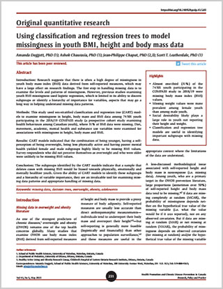
Interpreting the CART models

Sex-stratified results of the CART models are shown in Figures 1 to 3. Figures 1 presents results for BMI missingness, Figure 2 for body mass missingness and Figure 3 for height missingness. All CART models can be read starting from the root node (node 1) at the top of the tree, which contains all the training data for that particular dataset. Nodes underneath node 1 represent splits in the tree, whereby a split to the left is always a “yes” and a split to right is always a “no”; this applies to continuous and categorical variables. The label and colour of each node, “present” (green) or “missing” (blue), represents the situation that is more probable for data in that node. The shade of colour reflects the probabilities (darker colours indicate higher probability); probabilities are also included in each node, where left side shows the probability of being present, and the right side shows the probability of being missing. Variables that appear higher up the tree (i.e. closer to node 1) and those that appear more often can be considered more relevant criteria than variables that only appear once further down the tree.

For example, in the female BMI missingness CART model (Figures 1), the data are first split by weight perception. If individuals in this sample perceived their weight to be “about right” or underweight, they are in node 2. Node 2 contains 74% of the sample, and in this node the probability of missing BMI values is 0.27. If individuals perceived themselves to be overweight (i.e. the other remaining category for this variable), they are in node 3, which contains 26% of the data and where the probability of missing BMI values is 0.38. Similarly, for continuous variables, cut-offs are identified by the CART models. For example, in the female BMI missingness model the second node indicates that the model determined that 15 years of age was the cut-off that most differentiated the following sub-nodes.

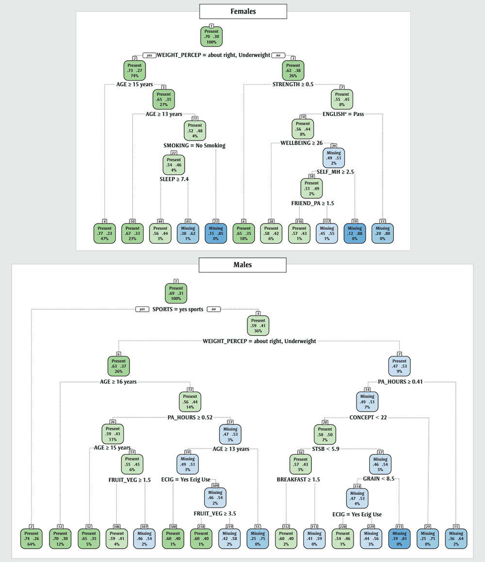
Figure 1 - Text description

Figure 1 comprises two smaller figures: one for females and one for males. Each figure is a set of nodes with data. The nodes are arranged in a binary way according to certain categories.

The following text description will describe the figure for females and then the figure for males will follow. Each figure requires three tables for its text description.

Figure 1 – Females – Text Equivalent Table 1

Node number	Node label and colour	Probability of BMI being present	Probability of BMI not being present	Percent of sample size	Category in which the node can be subdivided	Labels of nodes after subdivision for "yes" and "no," respectively
1	“Present” (green)	0.7	0.3	100%	WEIGHT_PERCEP = about right, Underweight	2, 3
2	“Present” (green)	0.73	0.27	74%	AGE ≥ 15	4, 5
3	“Present” (green)	0.62	0.38	26%	STRENGTH ≥ 0.5	6, 7
4	“Present” (green)	0.77	0.23	47%	(Not applicable - no other sub-nodes)	(Not applicable - no other sub-nodes)
5	“Present” (green)	0.65	0.35	27%	AGE ≥ 13	10, 11
6	“Present” (green)	0.65	0.35	18%	(Not applicable - no other sub-nodes)	(Not applicable - no other sub-nodes)
7	“Present” (green)	0.55	0.45	8%	ENGLISH = Pass	14, 15
10	“Present” (green)	0.67	0.33	23%	(Not applicable - no other sub-nodes)	(Not applicable - no other sub-nodes)
11	“Present” (green)	0.52	0.48	4%	SMOKING = No Smoking	22, 23
14	“Present” (green)	0.56	0.44	8%	WELLBEING ≥ 26	28, 29
15	“Missing” (blue)	0.2	0.8	0%	(Not applicable - no other sub-nodes)	(Not applicable - no other sub-nodes)
22	“Present” (green)	0.54	0.46	4%	SLEEP ≥ 7.4	44, 45
23	“Missing” (blue)	0.15	0.85	0%	(Not applicable - no other sub-nodes)	(Not applicable - no other sub-nodes)
28	“Present” (green)	0.58	0.42	6%	(Not applicable - no other sub-nodes)	(Not applicable - no other sub-nodes)
29	“Missing” (blue)	0.49	0.51	2%	SELF_MH ≥ 2.5	58, 59
44	“Present” (green)	0.56	0.44	3%	(Not applicable - no other sub-nodes)	(Not applicable - no other sub-nodes)
45	“Missing” (blue)	0.38	0.62	1%	(Not applicable - no other sub-nodes)	(Not applicable - no other sub-nodes)
58	“Present” (green)	0.51	0.49	2%	FRIEND_PA ≥ 1.5	116, 117
59	“Missing” (blue)	0.12	0.88	0%	(Not applicable - no other sub-nodes)	(Not applicable - no other sub-nodes)
116	“Present” (green)	0.57	0.43	1%	(Not applicable - no other sub-nodes)	(Not applicable - no other sub-nodes)
117	“Missing” (blue)	0.45	0.55	1%	(Not applicable - no other sub-nodes)	(Not applicable - no other sub-nodes)

The following table describes the binary variables of each of the node numbers in the preceding table. “Yes” means the node includes that category; “no” indicates the other remaining category. “N/A” means the node is not reached by that category as a parent node (e.g. because it is the root node, or is the node furthest away from the root node, or because it in another region of the model, etc.)

Figure 1 – Females – Text Equivalent Table 2

Node number	WEIGHT_PERCEP = about right, Underweight	AGE ≥ 15	AGE ≥ 13	SMOKING = No Smoking	SLEEP ≥ 7.4	STRENGTH ≥ 0.5	ENGLISH = Pass	WELLBEING ≥ 26	SELF_MH ≥ 2.5	FRIEND_PA ≥ 1.5
1	N/A	N/A	N/A	N/A	N/A	N/A	N/A	N/A	N/A	N/A
2	Yes	N/A	N/A	N/A	N/A	N/A	N/A	N/A	N/A	N/A
3	No	N/A	N/A	N/A	N/A	N/A	N/A	N/A	N/A	N/A
4	Yes	Yes	N/A	N/A	N/A	N/A	N/A	N/A	N/A	N/A
5	Yes	No	N/A	N/A	N/A	N/A	N/A	N/A	N/A	N/A
6	No	N/A	N/A	N/A	N/A	Yes	N/A	N/A	N/A	N/A
7	No	N/A	N/A	N/A	N/A	No	N/A	N/A	N/A	N/A
10	Yes	No	Yes	N/A	N/A	N/A	N/A	N/A	N/A	N/A
11	Yes	No	No	N/A	N/A	N/A	N/A	N/A	N/A	N/A
14	No	N/A	N/A	N/A	N/A	No	Yes	N/A	N/A	N/A
15	No	N/A	N/A	N/A	N/A	No	No	N/A	N/A	N/A
22	Yes	No	No	Yes	N/A	N/A	N/A	N/A	N/A	N/A
23	Yes	No	No	No	N/A	N/A	N/A	N/A	N/A	N/A
28	No	N/A	N/A	N/A	N/A	No	Yes	Yes	N/A	N/A
29	No	N/A	N/A	N/A	N/A	No	Yes	No	N/A	N/A
44	Yes	No	No	Yes	Yes	N/A	N/A	N/A	N/A	N/A
45	Yes	No	No	Yes	No	N/A	N/A	N/A	N/A	N/A
58	No	N/A	N/A	N/A	N/A	No	Yes	No	Yes	N/A
59	No	N/A	N/A	N/A	N/A	No	Yes	No	No	N/A
116	No	N/A	N/A	N/A	N/A	No	Yes	No	Yes	Yes
117	No	N/A	N/A	N/A	N/A	No	Yes	No	Yes	No

The following table describes the how far away each category is from the root node. For example, the number “2” would mean that the category is two branches away from the root node (node 1).

Figure 1 – Females – Text Equivalent Table 3

Name of category	Distance from root node
WEIGHT_PERCEP = about right, Underweight	1
AGE ≥ 15	2
STRENGTH ≥ 0.5	2
AGE ≥ 13	3
ENGLISH = Pass	3
SMOKING = No Smoking	4
WELLBEING ≥ 26	4
SLEEP ≥ 7.4	5
SELF_MH ≥ 2.5	5
FRIEND_PA ≥ 1.5	6

Figure 1 – Males – Text Equivalent Table 1

Node number	Node label and colour	Probability of BMI being present	Probability of BMI not being present	Percent of sample size	Category in which the node can be subdivided	Labels of nodes after subdivision for "yes" and "no," respectively
1	“Present” (green)	0.69	0.31	100%	SPORTS = yes sports	2, 3
2	“Present” (green)	0.74	0.26	64%	(Not applicable - no other sub-nodes)	(Not applicable - no other sub-nodes)
3	“Present” (green)	0.59	0.41	36%	WEIGHT_PERCEP = about right, Underweight	6, 7
6	“Present” (green)	0.63	0.37	26%	AGE ≥ 16	12, 13
7	“Missing” (blue)	0.47	0.53	9%	PA_HOURS ≥ 0.41	14, 15
12	“Present” (green)	0.7	0.3	12%	(Not applicable - no other sub-nodes)	(Not applicable - no other sub-nodes)
13	“Present” (green)	0.56	0.44	14%	PA_HOURS ≥ 0.52	26, 27
14	“Missing” (blue)	0.49	0.51	7%	CONCEPT < 22	28, 29
15	“Missing” (blue)	0.36	0.64	2%	(Not applicable - no other sub-nodes)	(Not applicable - no other sub-nodes)
26	“Present” (green)	0.59	0.41	11%	AGE ≥ 15	52, 53
27	“Missing” (blue)	0.47	0.53	3%	AGE ≥ 13	54, 55
28	“Present” (green)	0.5	0.5	7%	STSB < 5.9	56, 57
29	“Missing” (blue)	0.25	0.75	0%	(Not applicable - no other sub-nodes)	(Not applicable - no other sub-nodes)
52	“Present” (green)	0.65	0.35	5%	(Not applicable - no other sub-nodes)	(Not applicable - no other sub-nodes)
53	“Present” (green)	0.55	0.45	6%	FRUIT_VEG ≥ 1.5	106, 107
54	“Missing” (blue)	0.49	0.51	3%	ECIG = Yes Ecig Use	108, 109
55	“Missing” (blue)	0.25	0.75	0%	(Not applicable - no other sub-nodes)	(Not applicable - no other sub-nodes)
56	“Present” (green)	0.57	0.43	3%	BREAKFAST ≥ 1.5	112, 113
57	“Missing” (blue)	0.46	0.54	5%	GRAIN < 8.5	114, 115
106		0.59	0.41	4%	(Not applicable - no other sub-nodes)	(Not applicable - no other sub-nodes)
107	“Missing” (blue)	0.46	0.54	2%	(Not applicable - no other sub-nodes)	(Not applicable - no other sub-nodes)
108	“Present” (green)	0.6	0.4	1%	(Not applicable - no other sub-nodes)	(Not applicable - no other sub-nodes)
109	“Missing” (blue)	0.46	0.54	2%	FRUIT_VEG ≥ 3.5	218, 219
112	“Present” (green)	0.6	0.4	2%	(Not applicable - no other sub-nodes)	(Not applicable - no other sub-nodes)
113	“Missing” (blue)	0.41	0.59	0%	(Not applicable - no other sub-nodes)	(Not applicable - no other sub-nodes)
114	“Missing” (blue)	0.47	0.53	4%	ECIG = Yes Ecig Use	228, 229
115	“Missing” (blue)	0.19	0.81	0%	(Not applicable - no other sub-nodes)	(Not applicable - no other sub-nodes)
218	“Present” (green)	0.6	0.4	1%	(Not applicable - no other sub-nodes)	(Not applicable - no other sub-nodes)
219	“Missing” (blue)	0.42	0.58	2%	(Not applicable - no other sub-nodes)	(Not applicable - no other sub-nodes)
228	“Present” (green)	0.54	0.46	1%	(Not applicable - no other sub-nodes)	(Not applicable - no other sub-nodes)
229	“Missing” (blue)	0.44	0.56	3%	(Not applicable - no other sub-nodes)	(Not applicable - no other sub-nodes)

The following table describes the binary variables of each of the node numbers in the preceding table. “Yes” means the node includes that category; “no” indicates the other remaining category. “N/A” means the node is not reached by that category as a parent node (e.g. because it is the root node, or is the node furthest away from the root node, or because it in another region of the model.)

Figure 1 – Males – Text Equivalent Table 2

Node number	SPORTS = yes sports	WEIGHT_PERCEP = about right, Underweight	AGE ≥ 16	PA_HOURS ≥ 0.41	PA_HOURS ≥ 0.52	CONCEPT < 22	AGE ≥ 15	AGE ≥ 13	STSB < 5.9	FRUIT_VEG ≥ 1.5	ECIG = Yes Ecig Use	BREAKFAST ≥ 1.5	GRAIN< 8.5	FRUIT_VEG ≥ 3.5	ECIG = Yes Ecig Use
1	N/A	N/A	N/A	N/A	N/A	N/A	N/A	N/A	N/A	N/A	N/A	N/A	N/A	N/A	N/A
3	No	N/A	N/A	N/A	N/A	N/A	N/A	N/A	N/A	N/A	N/A	N/A	N/A	N/A	N/A
6	No	Yes	N/A	N/A	N/A	N/A	N/A	N/A	N/A	N/A	N/A	N/A	N/A	N/A	N/A
7	No	No	N/A	N/A	N/A	N/A	N/A	N/A	N/A	N/A	N/A	N/A	N/A	N/A	N/A
13	No	Yes	No	N/A	N/A	N/A	N/A	N/A	N/A	N/A	N/A	N/A	N/A	N/A	N/A
14	No	No	N/A	Yes	N/A	N/A	N/A	N/A	N/A	N/A	N/A	N/A	N/A	N/A	N/A
15	No	No	N/A	No	N/A	N/A	N/A	N/A	N/A	N/A	N/A	N/A	N/A	N/A	N/A
26	No	Yes	No	Yes	N/A	N/A	N/A	N/A	N/A	N/A	N/A	N/A	N/A	N/A	N/A
27	No	Yes	No	No	N/A	N/A	N/A	N/A	N/A	N/A	N/A	N/A	N/A	N/A	N/A
28	No	No	N/A	Yes	N/A	Yes	N/A	N/A	N/A	N/A	N/A	N/A	N/A	N/A	N/A
53	No	Yes	No	Yes	N/A	N/A	Yes	N/A	N/A	N/A	N/A	N/A	N/A	N/A	N/A
54	No	Yes	No	No	N/A	N/A	N/A	N/A	N/A	N/A	N/A	N/A	N/A	N/A	N/A
56	No	No	N/A	Yes	N/A	Yes	N/A	N/A	Yes	N/A	N/A	N/A	N/A	N/A	N/A
57	No	No	N/A	Yes	N/A	Yes	N/A	N/A	No	N/A	N/A	N/A	N/A	N/A	N/A
109	No	Yes	No	No	N/A	N/A	N/A	N/A	N/A	N/A	No	N/A	N/A	N/A	N/A
114	No	No	N/A	Yes	N/A	Yes	N/A	N/A	No	N/A	N/A	N/A	Yes	N/A	N/A
2	Yes	N/A	N/A	N/A	N/A	N/A	N/A	N/A	N/A	N/A	N/A	N/A	N/A	N/A	N/A
12	No	Yes	Yes	N/A	N/A	N/A	N/A	N/A	N/A	N/A	N/A	N/A	N/A	N/A	N/A
52	No	Yes	No	Yes	N/A	N/A	Yes	N/A	N/A	N/A	N/A	N/A	N/A	N/A	N/A
106	No	Yes	No	Yes	N/A	N/A	Yes	N/A	N/A	Yes	N/A	N/A	N/A	N/A	N/A
107	No	Yes	No	Yes	N/A	N/A	Yes	N/A	N/A	No	N/A	N/A	N/A	N/A	N/A
108	No	Yes	No	No	N/A	N/A	N/A	N/A	N/A	N/A	Yes	N/A	N/A	N/A	N/A
218	No	Yes	No	No	N/A	N/A	N/A	N/A	N/A	N/A	No	N/A	N/A	Yes	N/A
219	No	Yes	No	No	N/A	N/A	N/A	N/A	N/A	N/A	No	N/A	N/A	No	N/A
55	No	Yes	No	No	N/A	N/A	N/A	No	N/A	N/A	N/A	N/A	N/A	N/A	N/A
112	No	No	N/A	Yes	N/A	Yes	N/A	N/A	Yes	N/A	N/A	Yes	N/A	N/A	N/A
113	No	No	N/A	Yes	N/A	Yes	N/A	N/A	Yes	N/A	N/A	No	N/A	N/A	N/A
228	No	No	N/A	Yes	N/A	Yes	N/A	N/A	No	N/A	Yes	N/A	Yes	N/A	N/A
229	No	No	N/A	Yes	N/A	Yes	N/A	N/A	No	N/A	No	N/A	Yes	N/A	N/A
115	No	No	N/A	Yes	N/A	Yes	N/A	N/A	No	N/A	N/A	N/A	No	N/A	N/A
29	No	No	N/A	Yes	N/A	N/A	N/A	N/A	N/A	N/A	N/A	N/A	N/A	N/A	N/A
15	No	No	N/A	No	N/A	N/A	N/A	N/A	N/A	N/A	N/A	N/A	N/A	N/A	N/A

The following table describes the how far away each category is from the root node. For example, the number “2” would mean that the category is two branches away from the root node (node 1).

Figure 1 – Males – Text Equivalent Table 3

Name of category (binary variable)	Distance from root node
SPORTS = yes sports	1
WEIGHT_PERCEP = about right, Underweight	2
AGE ≥ 16	3
PA_HOURS ≥ 0.41	3
PA_HOURS ≥ 0.52	4
CONCEPT < 22	4
AGE ≥ 15	5
AGE ≥ 13	5
STSB < 5.9	5
FRUIT_VEG ≥ 1.5	6
ECIG = Yes Ecig Use	6
BREAKFAST ≥ 1.5	6
GRAIN < 8.5	6
FRUIT_VEG ≥ 3.5	7
ECIG = Yes Ecig Use	7

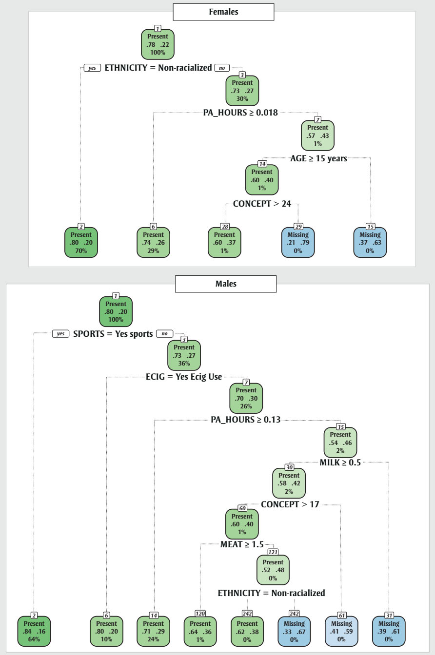
Figure 2 - Text description

Figure 2 comprises two smaller figures: one for females and one for males. Each figure is a set of nodes with data. The nodes are arranged in a binary way according to certain categories.

The following text description will describe the figure for females and then the figure for males will follow. Each figure requires three tables for its text description.

Figure 2 – Females – Text Equivalent Table 1

Node number	Node label and colour	Probability of BMI being present	Probability of BMI not being present	Percent of sample size	Category in which the node can be subdivided	Labels of nodes after subdivision for "yes" and "no," respectively
1	“Present” (green)	0.78	0.22	100%	ETHNICITY = Non-racialized	2, 3
2	“Present” (green)	0.8	0.2	70%	N/A	N/A
3	“Present” (green)	0.73	0.27	30%	PA_HOURS ≥ 0.018	6, 7
6	“Present” (green)	0.74	0.26	29%	N/A	N/A
7	“Present” (green)	0.57	0.43	1%	AGE ≥ 15	14, 15
14	“Present” (green)	0.6	0.4	1%	CONCEPT > 24	28, 29
28	“Present” (green)	0.6	0.37	1%	N/A	N/A
29	“Missing” (blue)	0.21	0.79	0%	N/A	N/A
15	“Missing” (blue)	0.37	0.63	0%	N/A	N/A

The following table describes the binary variables of each of the node numbers in the preceding table. “Yes” means the node includes that category; “no” indicates the other remaining category. “N/A” means the node is not reached by that category as a parent node (e.g. because it is the root node, or is the node furthest away from the root node, or because it in another region of the model, etc.)

Figure 2 – Females – Text Equivalent Table 2

Node number	ETHNICITY = Non-racialized	PA_HOURS ≥ 0.018	AGE ≥ 15	CONCEPT > 24
1	N/A	N/A	N/A	N/A
2	Yes	N/A	N/A	N/A
3	No	N/A	N/A	N/A
6	No	Yes	N/A	N/A
7	No	No	N/A	N/A
14	No	No	Yes	N/A
28	No	No	Yes	Yes
29	No	No	Yes	No
15	No	No	Yes	N/A

The following table describes the how far away each category is from the root node. For example, the number “2” would mean that the category is two branches away from the root node (node 1).

Figure 2 – Females – Text Equivalent Table 3

Name of category	Distance from root node
ETHNICITY = Non-racialized	1
PA_HOURS ≥ 0.018	2
AGE ≥ 15	3
CONCEPT > 24	4

Figure 2 – Males – Text Equivalent Table 1

Node number	Node label and colour	Probability of BMI being present	Probability of BMI not being present	Percent of sample size	Category in which the node can be subdivided	Labels of nodes after subdivision for "yes" and "no," respectively
1	“Present” (green)	0.78	0.22	100%	SPORTS = Yes sports	2, 3
2	“Present” (green)	0.8	0.2	70%	N/A	N/A
3	“Present” (green)	0.73	0.27	30%	ECIG = Yes Ecig Use	6, 7
6	“Present” (green)	0.8	0.2	10%	N/A	N/A
7	“Present” (green)	0.7	0.3	26%	PA_HOURS ≥ 0.13	14, 15
14	“Present” (green)	0.71	0.29	24%	N/A	N/A
15	“Present” (green)	0.54	0.46	2%	MILK ≥ 0.5	30, 31
30	“Present” (green)	0.58	0.42	2%	CONCEPT > 17	60, 61
31	“Missing” (blue)	0.39	0.61	0%	N/A	N/A
60	“Present” (green)	0.6	0.4	1%	MEAT ≥ 1.5	120, 121
61	“Present” (green)	0.41	0.59	0%	N/A	N/A
120	“Present” (green)	0.64	0.36	1%	N/A	N/A
121	“Present” (green)	0.52	0.48	0%	ETHNICITY = Non-recialized	242, 243
242	“Missing” (blue)	0.62	0.38	0%	N/A	N/A
243	“Missing” (blue)	0.33	0.67	0%	N/A	N/A

The following table describes the binary variables of each of the node numbers in the preceding table. “Yes” means the node includes that category; “no” indicates the other remaining category. “N/A” means the node is not reached by that category as a parent node (e.g. because it is the root node, or is the node furthest away from the root node, or because it in another region of the model.)

Figure 2 – Males – Text Equivalent Table 2

Node number	SPORTS = Yes sports	ECIG = Yes Ecig Use	PA_HOURS ≥ 0.13	MILK ≥ 0.5	CONCEPT > 17	MEAT ≥ 1.5	ETHNICITY = Non-recialized
1	N/A	N/A	N/A	N/A	N/A	N/A	N/A
2	Yes	N/A	N/A	N/A	N/A	N/A	N/A
3	No	N/A	N/A	N/A	N/A	N/A	N/A
6	No	Yes	N/A	N/A	N/A	N/A	N/A
7	No	No	N/A	N/A	N/A	N/A	N/A
14	No	No	Yes	N/A	N/A	N/A	N/A
15	No	No	No	N/A	N/A	N/A	N/A
30	No	No	No	Yes	N/A	N/A	N/A
31	No	No	No	No	N/A	N/A	N/A
60	No	No	No	Yes	Yes	N/A	N/A
61	No	No	No	Yes	No	N/A	N/A
120	No	No	No	Yes	Yes	Yes	N/A
121	No	No	No	Yes	Yes	No	N/A
242	No	No	No	Yes	Yes	Yes	Yes
243	No	No	No	Yes	Yes	Yes	No

The following table describes the how far away each category is from the root node. For example, the number “2” would mean that the category is two branches away from the root node (node 1).

Figure 2 – Males – Text Equivalent Table 3

Name of category (binary variable)	Distance from root node
SPORTS = Yes sports	1
ECIG = Yes Ecig Use	2
PA_HOURS ≥ 0.13	3
MILK ≥ 0.5	4
CONCEPT > 17	5
MEAT ≥ 1.5	6
ETHNICITY = Non-recialized	7

 

Figure 3 - Text description

Figure 3 comprises two smaller figures: one for females and one for males. Each figure is a set of nodes with data. The nodes are arranged in a binary way according to certain categories.

The following text description will describe the figure for females and then the figure for males will follow. Each figure requires three tables for its text description.

Figure 3 – Females – Text Equivalent Table 1

Node number	Node label and colour	Probability of BMI being present	Probability of BMI not being present	Percent of sample size	Category in which the node can be subdivided	Labels of nodes after subdivision for "yes" and "no," respectively
1	“Present” (green)	0.85	0.15	100%	AGE ≥ 14	2, 3
2	“Present” (green)	0.87	0.13	86%	N/A	N/A
3	“Present” (green)	0.62	0.38	26%	AGE ≥ 13	6, 7
6	“Present” (green)	0.74	0.26	9%	N/A	N/A
7	“Present” (green)	0.64	0.63	5%	CANNABIS = No Cannabis Use	14, 15
14	“Present” (green)	0.65	0.35	5%	N/A	N/A
15	“Missing” (blue)	0.24	0.76	0%	N/A	N/A

The following table describes the binary variables of each of the node numbers in the preceding table. “Yes” means the node includes that category; “no” indicates the other remaining category. “N/A” means the node is not reached by that category as a parent node (e.g. because it is the root node, or is the node furthest away from the root node, or because it in another region of the model, etc.)

Figure 3 – Females – Text Equivalent Table 2

Node number	AGE ≥ 14	AGE ≥ 13	CANNABIS = No Cannabis Use
1	N/A	N/A	N/A
2	Yes	N/A	N/A
3	No	N/A	N/A
6	No	Yes	N/A
7	No	No	N/A
14	No	No	Yes
15	No	No	No

The following table describes the how far away each category is from the root node. For example, the number “2” would mean that the category is two branches away from the root node (node 1).

Figure 3 – Females – Text Equivalent Table 3

Name of category	Distance from root node
AGE ≥ 14	1
AGE ≥ 13	2
CANNABIS = No Cannabis Use	3

Figure 3 – Males – Text Equivalent Table 1

Node number	Node label and colour	Probability of BMI being present	Probability of BMI not being present	Percent of sample size	Category in which the node can be subdivided	Labels of nodes after subdivision for "yes" and "no," respectively
1	“Present” (green)	0.81	0.19	100%	AGE ≥ 14	2, 3
2	“Present” (green)	0.83	0.17	87%	N/A	N/A
3	“Present” (green)	0.67	0.33	13%	SPORTS = yes sports	6, 7
6	“Present” (green)	0.7	0.3	9%	N/A	N/A
7	“Present” (green)	0.59	0.41	4%	FRUIT_VEG ≥ 2.5	14, 15
14	“Present” (green)	0.64	0.36	2%	PA_HOURS ≥ 0.13	28, 29
15	“Present” (green)	0.53	0.47	2%	MILK ≥ 1.5	30, 31
28	“Present” (green)	0.66	0.34	2%	N/A	N/A
29	“Missing” (blue)	0.42	0.58	0%	N/A	N/A
30	“Present” (green)	0.58	0.42	1%	MEAT ≥ 1.5	60, 61
31	“Missing” (blue)	0.46	0.54	1%	AGE ≥ 13	62, 63
60	“Present” (green)	0.62	0.37	1%	N/A	N/A
61	“Present” (green)	0.5	0.5	0%	PA_HOURS < 1.3	122, 123
122	“Present” (green)	0.57	0.43	0%	AGE ≥ 13	244, 245
123	“Missing” (blue)	0.36	0.68	0%	N/A	N/A
244	“Present” (green)	0.65	0.35	0%	N/A	N/A
245	“Missing” (blue)	0.37	0.62	0%	N/A	N/A
62	“Present” (green)	0.51	0.49	1%	SLEEP < 6.3	124, 125
63	“Missing” (blue)	0.33	0.67	0%	N/A	N/A
124	“Present” (green)	0.78	0.22	0%	N/A	N/A
125	“Missing” (blue)	0.47	0.53	0%	FAST_FOOD < 1.5	250, 251
250	“Present” (green)	0.51	0.49	0%	PA_HOURS ≥ 1.7	500, 501
251	“Missing” (blue)	0.31	0.69	0%	N/A	N/A
500	“Present” (green)	0.73	0.27	0%	N/A	N/A
501	“Missing” (blue)	0.45	0.55	0%	N/A	N/A

The following table describes the binary variables of each of the node numbers in the preceding table. “Yes” means the node includes that category; “no” indicates the other remaining category. “N/A” means the node is not reached by that category as a parent node (e.g. because it is the root node, or is the node furthest away from the root node, or because it in another region of the model.)

Figure 3 – Males – Text Equivalent Table 2

Node number	AGE ≥ 14	SPORTS = yes sports	FRUIT_VEG  ≥ 2.5	PA_HOURS ≥ 0.13	MILK ≥ 1.5	MEAT ≥ 1.5	AGE ≥ 13	PA_HOURS < 1.3	AGE ≥ 13	SLEEP < 6.3	FAST_FOOD < 1.5	PA_HOURS ≥ 1.7
1	N/A	N/A	N/A	N/A	N/A	N/A	N/A	N/A	N/A	N/A	N/A	N/A
2	Yes	N/A	N/A	N/A	N/A	N/A	N/A	N/A	N/A	N/A	N/A	N/A
3	No	N/A	N/A	N/A	N/A	N/A	N/A	N/A	N/A	N/A	N/A	N/A
6	No	Yes	N/A	N/A	N/A	N/A	N/A	N/A	N/A	N/A	N/A	N/A
7	No	No	N/A	N/A	N/A	N/A	N/A	N/A	N/A	N/A	N/A	N/A
14	No	No	Yes	N/A	N/A	N/A	N/A	N/A	N/A	N/A	N/A	N/A
15	No	No	No	N/A	N/A	N/A	N/A	N/A	N/A	N/A	N/A	N/A
28	No	No	Yes	Yes	N/A	N/A	N/A	N/A	N/A	N/A	N/A	N/A
29	No	No	Yes	No	N/A	N/A	N/A	N/A	N/A	N/A	N/A	N/A
30	No	No	No	N/A	Yes	N/A	N/A	N/A	N/A	N/A	N/A	N/A
31	No	No	No	N/A	No	N/A	N/A	N/A	N/A	N/A	N/A	N/A
60	No	No	No	N/A	Yes	Yes	N/A	N/A	N/A	N/A	N/A	N/A
61	No	No	No	N/A	Yes	No	N/A	N/A	N/A	N/A	N/A	N/A
122	No	No	No	N/A	Yes	No	N/A	Yes	N/A	N/A	N/A	N/A
123	No	No	No	N/A	Yes	No	N/A	No	N/A	N/A	N/A	N/A
244	No	No	No	N/A	Yes	No	N/A	Yes	Yes	N/A	N/A	N/A
245	No	No	No	N/A	Yes	No	N/A	Yes	No	N/A	N/A	N/A
62	No	No	No	N/A	No	N/A	N/A	N/A	Yes	N/A	N/A	N/A
63	No	No	No	N/A	No	N/A	N/A	N/A	No	N/A	N/A	N/A
124	No	No	No	N/A	No	N/A	N/A	N/A	Yes	Yes	N/A	N/A
125	No	No	No	N/A	No	N/A	N/A	N/A	Yes	No	N/A	N/A
250	No	No	No	N/A	No	N/A	N/A	N/A	Yes	No	Yes	N/A
251	No	No	No	N/A	No	N/A	N/A	N/A	Yes	No	No	N/A
500	No	No	No	N/A	No	N/A	N/A	N/A	Yes	No	Yes	Yes
501	No	No	No	N/A	No	N/A	N/A	N/A	Yes	No	Yes	No

The following table describes the how far away each category is from the root node. For example, the number “2” would mean that the category is two branches away from the root node (node 1).

Figure 3 – Males – Text Equivalent Table 3

Name of category (binary variable)	Distance from root node
AGE ≥ 14	1
SPORTS = yes sports	2
FRUIT_VEG ≥ 2.5	3
PA_HOURS ≥ 0.13	4
MILK ≥ 1.5	4
MEAT ≥ 1.5	5
AGE ≥ 13	5
PA_HOURS < 1.3	6
AGE ≥ 13	7
SLEEP < 6.3	6
FAST_FOOD < 1.5	7
PA_HOURS ≥ 1.7	8

CART model accuracy

Accuracy testing using the test partition of the dataset showed that all models became more accurate after pruning. Pruned accuracy of CART BMI models was 69% for females and 70% for males, of CART body mass models was 78% for females and 80% for males and of CART height models was 85% for females and 81% for males.

Discussion

This study used a decision tree approach to examine missingness in BMI, height and body mass in a large sample of Canadian youth. One of the aims of this study was to inform the structure of missingness in these variables, as youth self-reported height and body mass can be missing in large proportions and published examinations of this missingness are lacking. The other aim of this study was to employ a newer decision tree method to examining missingness in a dataset in order to overcome some of the barriers of regression-based approaches.

When we previously examined missing BMI, height and body mass data in this sample using a regression approach,^{Footnote 15} we found that more information was needed on the structure of missingness and hierarchy of the importance of variables. The decision tree approach used in this study yielded insights into the mechanisms of missingness in this sample that can inform future studies on youth OWOB.

Mechanisms of BMI, height and body mass missingness

In the BMI missingness CART models we developed, age and weight perception were among the first few primary splits for both males and females. Previous research has suggested that individuals who are younger are more likely to be missing BMI values because they don’t know their own height and body mass;^{Footnote 26} this is consistent with the CART models, as each split by age led to a node with a higher likelihood of missingness for the younger groups. Weight perception consistently split those who perceived themselves as overweight from their “about right” and underweight counterparts, leading to a higher likelihood of missingness in the group who perceived themselves as overweight. Previous studies examining BMI missingness mechanisms did not include a measure of weight perception, but two studies have found that poorer body satisfaction was associated with greater likelihood of missing BMI values.^{Footnote 14Footnote 27}

Physical activity was also one of the first few splits in both the male and female models. In the female model, strength training was identified as important split criteria, where individuals who did not do any strength training were more likely on average to be missing BMI values. A similar mechanism was observed for males, but with sports and hours of physical activity; not playing sports or being, on average, less physically active each day led to splits where the likelihood of missing BMI values was greater. This is consistent with previous research that included some measures of physical activity.^{Footnote 6Footnote 7Footnote 14}

Mental health–related variables also appeared in both male and female models. For females, well-being and self-rated mental health were used for splitting, and for males, self-concept was used. For all these mental health–related variables, lower scores (i.e. scores indicating poorer mental health) were associated with a greater likelihood of missing BMI values.

The consistent splitting of individuals who perceived themselves as overweight into a separate group more likely to be missing BMI values suggests that those with a higher BMI were more likely to be nonreporters. Notably, weight perception cannot be assumed as a direct proxy for BMI or body mass because youth may miscategorize themselves;^{Footnote 28Footnote 29Footnote 30} however, weight perception may be considered alongside other factors to determine which missingness pattern is most probable.

Findings related to physical activity support the idea that individuals missing BMI values are more likely to have a higher BMI, as those who are less physically active were also split into groups more likely to be missing BMI values, and inverse associations between physical activity and BMI are well-established.^{Footnote 31Footnote 32} These findings, along with what we know about heightened body image concerns during adolescence,^{Footnote 33} demonstrate that social desirability may be playing a role in youth nonreporting of height and body mass in this sample.

Height and body mass missingness CART models had some split criteria similar to those of the BMI missingness models, with age a common partitioning variable and physical activity, diet, mental health and substance use variables also observed. One finding exclusive to the body mass missingness models was ethnicity: the model indicated that racialized individuals were more likely to be missing body mass values. Interestingly, although weight perception was identified as a key variable for BMI missingness, it was not identified as important in the body mass missingness CART models for males and females.

Utility of CART in examining BMI, height and body mass missingness

The decision tree approach used in this study to examine missingness appears to have several advantages over traditional regression approaches. The visual nature of decision tree models makes them particularly useful for understanding how missingness might be influenced by other variables. For example, the inclusion and directions of splitting related to weight perception, physical activity and mental health in the CART models suggest that the missingness in BMI may be not missing at random because missing data appear more likely among those with a higher BMI. While not missing at random is not a provable phenomenon, the CART models provide evidence against a missing-completely-at-random mechanism, as several subgroups who are highly likely to be missing BMI were identified based on observed covariates.^{Footnote 34} Future OWOB research should consider the mechanisms and degree of missingness in BMI, and where examinations indicate that data may be missing at random or not missing at random, certain statistical approaches (e.g. complete case analysis) may not be ideal because of the risk of bias.^{Footnote 9}

While a regression model could similarly highlight the associations between predictor variables and BMI missingness (e.g. observing a positive odds ratio for self-perception as overweight), one advantage of the CART models is the easily observed hierarchy of the importance of variables. In the BMI CART model, weight perception being among the top two splits for males and females indicates that this variable is of primary importance in predicting BMI missingness. We previously examined BMI missingness using regression;^{Footnote 15} while weight perception was significantly associated with missingness, it was only one of many significant variables and relative importance couldn’t be empirically discerned.

Another advantage of CART models is that one can follow through a decision tree order to identify important subgroups. For example, in the male BMI missingness tree, the 9% of this sample who did not participate in sports and perceived themselves as overweight were more likely than not to be missing BMI values. Moreover, following subgroups to the bottom of the trees reveals that, overall, individuals who perceive themselves as overweight and who were worse off in terms of their physical activity, dietary behaviours, academics and mental health are almost certain to be missing BMI values. In other words, CART models identified that those in the complete sample (i.e. those not missing BMI data) were physically, emotionally and mentally healthier than their counterparts with missing data. As such, a complete case analysis approach on these data would certainly be biased, potentially leading to incorrect research conclusions and inappropriate related policy and programming recommendations.

Examining missing data is often the first step in certain statistical approaches, such as multiple imputation. Although such examinations are needed to identify auxiliary variables that can inform reasonable imputed values, selecting these variables can be difficult if there are many variables related to missingness. This was the case with our previous work using regression; almost all variables were significantly associated with missingness in BMI, height and body mass, and comparing the effective sizes would not have been appropriate as these variables use different scales.^{Footnote 15}

The hierarchical nature of CART models makes the process of selecting auxiliary variables more systematic. For example, CART models can parse out redundant variables; while previous regression work identified weight goal as significantly related to BMI missingness,^{Footnote 15} the CART models in this study did not perform any splits based on this variable, possibly because BMI missingness is sufficiently explained by the weight perception variable alone.

In this study we demonstrated the utility of using CART models to examine missingness in youth height, body mass and BMI. However, missingness is pervasive, and a similar approach may be useful in many other applied research domains. Moreover, public availability of machine-learning packages in R as well as a wealth of online resources make this approach reasonably accessible and feasible for applied researchers.

Conclusion

This study adds to the limited existing research examining missingness in youth BMI, height and body mass data. CART models demonstrated that age, self-perception as overweight, lower physical activity and poorer mental health identified the subgroups most likely to be missing BMI values. The direction of model partitioning for these variables suggests that youth with higher BMI may be more likely to be missing BMI values and that deleting missing cases in an analysis would likely lead to biased findings.

Future research using youth self-reported data may find that CART models are a particularly useful tool for examining missingness and help select a statistical approach appropriate for handling missing data.

Acknowledgements

The COMPASS study has been supported by a bridge grant from the Canadian Institutes of Health Research (CIHR) Institute of Nutrition, Metabolism and Diabetes (INMD) through the “Obesity – Interventions to Prevent or Treat” priority funding awards (OOP-110788; awarded to SL); an operating grant from the CIHR Institute of Population and Public Health (IPPH) (MOP-114875; awarded to SL); a CIHR project grant (PJT-148562; awarded to SL); a CIHR bridge grant (PJT-149092; awarded to KP/SL); a CIHR project grant (PJT-159693; awarded to KP); a research funding arrangement with Health Canada (#1617-HQ-000012; contract awarded to SL); and a CIHR–Canadian Centre on Substance Abuse and Addiction (CCSA) team grant (OF7 B1-PCPEGT 410-10-9633; awarded to SL).

A SickKids Foundation New Investigator Grant, in partnership with CIHR Institute of Human Development, Child and Youth Health (IHDCYH) (Grant No. NI21-1193; awarded to KAP), funds a mixed methods study examining the impact of the COVID-19 pandemic on youth mental health, leveraging COMPASS study data. The COMPASS-Quebec project also benefits from funding from the Ministère de la Santé et des Services sociaux of the province of Quebec, and the Direction régionale de santé publique du CIUSSS de la Capitale-Nationale.

Conflicts of interest

The authors report no conflicts of interest.

Authors’ contributions and statement

AD, AC, JPC and SL – Conceptualization; AD and AC – Methodology; AD – Formal analysis, Writing – Original draft; SL – Funding acquisition, Resources, Supervision; AD, AC, JPC and SL – Writing – Review and editing. All authors read and agreed upon the published version of the manuscript.

The content and views expressed in this article are those of the authors and do not necessarily reflect those of the Government of Canada.

Previous | Table of Contents | Next