
Chapter 2: Cancer incidence in Canada: trends and projections (1983-2032) - HPCDP: Volume 35, Supplement 1, Spring 2015
Chapter 2: Data and Methods
2.1 Data
The observed cancer incidence data used for the projections cover 1983 to 2007, which represents the most recent period for which data are available for all parts of Canada. We extracted data from the Canadian Cancer Registry (CCR) for 1992 to 2007 and from the National Cancer Incidence Reporting System (NCIRS) for the earlier years. While the CCR is a person oriented database, the NCIRS is an event oriented database with cases diagnosed from 1969 to 1991. The cases in the NCIRS were coded in or converted to the International Classification of Diseases, Ninth Revision (ICD-9).Endnote 6 Projections were prepared for the most frequent invasive primary cancers (including in situ bladder cancers but excluding non-melanoma skin cancer (i.e. basal and squamous carcinoma). We generally defined cancer cases based on the International Classification of Diseases for Oncology, Third Edition (ICD-O-3) and classified them using Surveillance, Epidemiology, and End Results (SEER) Program Incidence Site Recode shown in Table 2.1.Endnote 7, Endnote 8 Cases retrieved from the NCIRS used equivalent ICD-9 codes. Changes in cancer definition over time were derived following the methods outlined in the Canadian Cancer Statistics.Endnote 1
| Cancer | ICD-O-3 site/histology typeTable 2.1 - Footnote a (Incidence) |
|---|---|
| Oral | C00-C14 |
| Esophagus | C15 |
| Stomach | C16 |
| Colorectal | C18-C20, C26.0 |
| Liver | C22.0 |
| Pancreas | C25 |
| Larynx | C32 |
| Lung | C34 |
| Melanoma | C44 (Type 8720-8790) |
| Breast | C50 |
| Cervix | C53 |
| Body of uterus | C54-C55 |
| Ovary | C56.9 |
| Prostate | C61.9 |
| Testis | C62 |
| Kidney | C64.9, C65.9 |
| Bladder (including in situ) | C67 |
| Central nervous system | C70-C72 |
| Thyroid | C73.9 |
| Hodgkin lymphomaTable 2.1 - Footnote b | Type 9650-9667 |
| Non-Hodgkin lymphomaTable 2.1 - Footnote b | Type 9590-9596, 9670-9719, 9727-9729 Type 9823, all sites except C42.0,.1,.4 Type 9827, all sites except C42.0,.1,.4 |
| Multiple myelomaTable 2.1 - Footnote b | Type 9731, 9732, 9734 |
| LeukemiaTable 2.1 - Footnote b | Type 9733, 9742, 9800-9801, 9805, 9820, 9826, 9831-9837, 9840, 9860-9861, 9863, 9866-9867, 9870-9876, 9891, 9895-9897, 9910, 9920, 9930-9931, 9940, 9945-9946, 9948, 9963-9964 Type 9823 and 9827, sites C42.0,.1,.4 |
| All other cancers | All sites C00-C80, C97 not listed above |
| MesotheliomaTable 2.1 - Footnote b | 9050-9055 |
| Kaposi's sarcomaTable 2.1 - Footnote bTable 2.1 - Footnote c | 9140 |
| Small intestine | C17 |
| Anus | C21 |
| Gallbladder | C23 |
| Other digestive system | C22.1, C24, C26.8-9, C48 |
| Other respiratory system | C30-31, C33, C38.1-9, C39 |
| Bone and joints | C40-41 |
| Soft tissue (including heart) | C38.0, C47, C49 |
| Other skin | C44 excl. 8050:8084, 8090:8110, 8720:8790 |
| Other female genital system | C51-52, C57-58 |
| Penis | C60 |
| Other male genital system | C63 |
| Ureter | C66 |
| Other urinary system | C68 |
| Eye | C69 |
| Other endocrine | C37.9, C74, C75 |
| Other, ill-defined, and unknown | Type 9740, 9741, 9750-9758, 9760-9769, 9950-9962, 9970-9989; C76.0-76.8 (type 8000-9589); C80.9 (type 8000-9589); C42.0-42.4 (type 8000-9589); C77.0-C77.9 (type 8000-9589) |
| All cancers | All invasive sites |
|
|
Population estimates for Canada and the provinces/territories are based on quinquennial censuses conducted from 1981 to 2006. We used intercensal estimates prepared by Statistics Canada for the years between these censuses and postcensal estimates for 2007 to 2010.Endnote 9 Projected population estimates were used for 2011 to 2032, as prepared by Statistics Canada under assumptions of medium growth (scenario M1).Endnote 10 The scenario M1 incorporates medium growth and historical trends (1981-2008) of interprovincial migration. For the total population, the low and high growth scenarios are about 6% below and above the M1 scenario, but this range is reduced to 3% for ages 65 or older.
Data on cancer incidence counts and population estimates were summarized into 5-year age groups (0-4, 5-9,..., 80-84, 85+) and 5-year periods of diagnosis (1983-1987, 1988-1992, 1993-1997, 1998-2002, 2003-2007) by sex and geographical region (British Columbia, the Prairie provinces [Alberta, Saskatchewan and Manitoba] individually and together, Ontario, Quebec, the Atlantic provinces [New Brunswick, Prince Edward Island, Nova Scotia and Newfoundland and Labrador] individually and together, and the North [Yukon, Northwest Territories and Nunavut]). The projected population figures were similarly aggregated for 5 projection quinquennia (2008-2012, 2013-2017, 2018-2022, 2023- 2027, 2028-2032). The single-year data from 1994 to 2007 were used for projecting prostate cancer incidence. Rates for each category were calculated by dividing the number of cases in each category (a combination of cancer site, sex, region, period, and age group) by the corresponding population figure. These age-specific rates were standardized to the 1991 Canadian population (Table 2.2), using the direct method,Endnote 11 to obtain the age-standardized incidence rates (ASIRs).
| Age Group | Population (per 100 000) |
|---|---|
| 0-4 | 6946.40 |
| 5-9 | 6945.40 |
| 10-14 | 6803.40 |
| 15-19 | 6849.50 |
| 20-24 | 7501.60 |
| 25-29 | 8994.40 |
| 30-34 | 9240.00 |
| 35-39 | 8338.80 |
| 40-44 | 7606.30 |
| 45-49 | 5953.60 |
| 50-54 | 4764.90 |
| 55-59 | 4404.10 |
| 60-64 | 4232.60 |
| 65-69 | 3857.00 |
| 70-74 | 2965.90 |
| 75-79 | 2212.70 |
| 80-84 | 1359.50 |
| 85+ | 1023.70 |
| Total | 100 000.00 |
|
Data source: Census and Demographics Branch, Statistics Canada Note: The Canadian population distribution is based on the final postcensal estimates of the July 1, 1991, Canadian population, adjusted for census undercoverage. The age distribution of the population has been weighted and normalized. |
|
2.2 Methods
2.2.1 Projection methods
Future trends in cancer incidence rates are generally estimated by extending past trends using statistical models. A statistical model formulates the relationship between the risk factors and the cancer rates, and projections can be obtained by applying the future times in the equation.
There are several methods for projecting cancer burden, differing in terms of the type of model, selection of the data used for model fitting, and the method of extrapolating the model components into future periods. The model type diverges from simple linear or log-linear regression of age-specific rates or counts against timeEndnote 2, Endnote 12, Endnote 13 to age-period-cohort (APC) modelling. Endnote 11, Endnote 14, Endnote 15 Within the framework of APC models, effects of age, period and cohort are addressed in heterogeneous ways such as generalized linear modelsEndnote 16, Endnote 17 including their derivative, Nordpred method, based on a step function on 5-year intervals,Endnote 3, Endnote 15 generalized additive modelsEndnote 18, Endnote 19 with polynomial Endnote 15, Endnote 20 or spline smoothing methods,Endnote 21 and Bayesian modelsEndnote 22 with Markov chain Monte Carlo (MCMC) simulation.Endnote 23 The link function is either common exponential Endnote 11, Endnote 14, Endnote 22 or non-canonical power.Endnote 3, Endnote 15 A model is fitted to all available data or their subset for an adequate fit through a goodness- of-fit test.Endnote 3, Endnote 15 The assumptions used for extrapolating the observed trends include keeping current rates unchanged in future,Endnote 24 continuing overall historical trend,Endnote 2, Endnote 22 extending only the most recent trend,Endnote 3, Endnote 15 and adjusting the extent to which the observed trend are likely to influence the future.Endnote 3, Endnote 15 To develop the most accurate profile of future cancer burden, we used the major projection models to produce projections of current rates as would have been forecast 15 or 20 years ago based on the long-term data series in Canada, compared the projected rates with those observed, and concluded with a cancer-dependent modelling approach. This multiple modelling approach consists of the following models and integrates the strengths of these models.
The common projection models relate incidence to the 3 intrinsically interdependent time dimensions: age at diagnosis (age), year of diagnosis (period), and year of birth (cohort). The Nordpred APC modelEndnote 3, Endnote 15 uses the power-5 link function instead of the traditional logarithmic link to reduce the exponential changes; summarizes the linear trends in period and cohort over the observed data into a drift component and then arithmetically attenuates the drift into the future to damp the impact of past trends in the future; chooses data for model fitting; and chooses the drift for extrapolations. Nordpred with its standard and various modified parameter settings was the primary method used in the projections in this monograph. When cohort effects were not present, we considered a Nordpred model without cohort component as an alternative. When there were too few observed cases to properly estimate model parameters via the Nordpred method or projections from Nordpred seemed unlikely based on biological and clinical grounds, we pursued Bayesian APC modelsEndnote 22 or submodels with various prior settings, 5-year average method or applying a relative percentage adjustment to national estimates to obtain the estimates for a jurisdiction. Bayesian models estimate the age-specific rates from their posterior distribution through repeated iterative sampling. The 5-year average model assumes the current agespecific rates will remain in future. In addition, we used an age-specific trend power-5 model fitted to most recent data for the projections of prostate cancer to reduce the impact of prostate-specific antigen (PSA) screening on the long-term historical trend.
All the long-term projection models depend on an assumption of the continuity of past trends in age-specific rates, but with different extent. The details of these models, model section methods, and "best" models are described below.
2.2.1.1 Projection models
2.2.1.1.1 Nordpred power-5 models--modified generalized linear models (NP_ADPC and NP_ADP)
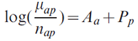
The Nordpred approach was developed as part of a comprehensive analysis of cancer trends in the Nordic countries.Endnote 3, Endnote 25 The approach is based on a standard APC Poisson regression modelEndnote 14, Endnote 16, Endnote 26 but has been shown to give more realistic predictions, especially for long-term projections. Endnote 15, Endnote 27 It is now one of the most frequently used methods for cancer projections worldwide.Endnote 28, Endnote 29, Endnote 30, Endnote 31 The log-linear relationship between the rate and the covariates in the standard model produces predictions in which the rates grow exponentiallywith time. Nordpred uses a powerlink function instead of the log-link function to lower this growth. The power-link function is an approximation of the log-link function based on Box-Cox power transformation theory, in which λ→ 0lim xλ = log(x). The Nordpred model is defined as
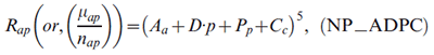
where Rap is the incidence rate for age group a in calendar period p, which is the mean count µap of caseap divided by the corresponding population size nap; Aa, Pp and Cc are the non-linear components of age group a, period p and cohort c, respectively; and D is the common linear drift parameter of period and cohort.26 A cohort is calculated by subtracting age from period: c = A +p - a, with A = number of age groups (i.e. 18).
To achieve an adequate fit of each data to the model, the number of 5-year periods on which the projections should be based is chosen in the Nordpred software by using a goodness-of-fit test to successively remove the earlier periods. To extrapolate the model for future periods, two approaches are considered instead of simple continuation of the overall historical trend. Firstly, the software determines whether the average trend across all observed values, or the slope for the last 10 years of observed values, is used as the drift component D to be projected. The software does this by testing for departure from a linear trend. If the trend across the entire observation period departs significantly from linearity, only the trend in the most recent 10 years is used for projection. The "recent" option in the software allows choosing between using the average trend (recent=F) or the trend for the last 10 years (recent=T). Secondly, to attenuate the impact of current trends in future periods, a "cut trend" (or "drift") option is used, which is a vector of proportions indicating how much to cut the trend estimate for each 5-year projection period. A gradual reduction in the drift parameter of 25%, 50%, 75% and 75% in the second, third, fourth and fifth 5- year period, respectively, is used as a default "cut" in Nordpred.Endnote 3, Endnote 25
To explore accurate projection methods for this study, we compared the power-5 models and Poisson models (using log link instead of the power link in equation NP_ADPC), with the Nordpred option recommendations and their modifications. The default "cut trend" vector was modified to reduce or increase the impact of current trend in future periods.
For each age group, a minimum of 5 cases in each 5-year period was required; for age groups below this limit, the average number of cases in the last 2 periods was used to calculate future rates. If a limit of 10 had been used, as in the report for Nordic countries in most of the situations, 3 a larger number of age groups would have been based on the average rates. This would reduce the effect of current trends, so a low limit of 5 was chosen as a trade-off between unbiased estimation of the underlying trend and a large estimation error.
In addition to the full ADPC model, we also considered using an age-drift-period model (ADP) with power-5 link functions for cancers with average annual counts of fewer than 50 over the last observed 5 years when cohort effects were not present based on a significance test:
This ADP model was used for rare cancers in Iceland in an analysis of cancer trends in the Nordic countries.Endnote 3
2.2.1.1.2 Bayesian Markov chain Monte Carlo method
Instead of a maximum likelihood approach, we applied a Bayesian framework to the APC model or submodel. The Bayesian method incorporates prior knowledge into the model to derive a posterior distribution and uses MCMC approximationsEndnote 22, Endnote 23 for inference (parameter estimates). We considered this approach for situations in which average annual count over the last observed 5 years was less than or equal to 10 (when there were too few observed cases to properly estimate model parameters via the Nordpred method) or if projections from Nordpred seemed unlikely. We considered 2 Bayesian approaches.
2.2.1.1.2.1 Bayesian APC model with autoregressive prior - Bray approach (B_APC)
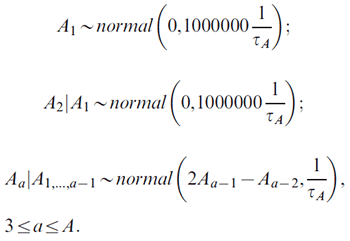
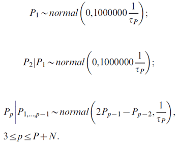
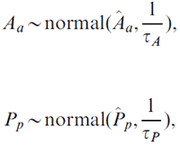
For the classical APC Poisson model,Endnote 26 Bray specified a second-order autoregressive prior model to smooth age, period and cohort effects and to extrapolate period and cohort effects.Endnote 22, Endnote 23 The model can be written as,
Supposing that we compute N-period projections based on P-period observed data, there are total C = A+P − 1 cohorts. With the Nordpred model, an individual cohort c can be calculated as c = A + p − a. The prior distributions are defined as follows. For the A age effects:
For the P + N period effects:
For the C + N cohort effects:
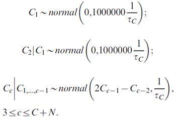
The variance parameters τA, τP and τC (determining the smoothness of age, period and cohort effects, respectively) are given the same gamma prior,
Fitted and projected rates are derived by combining the simulated age, period and cohort effects based on
Rap = exp(Aa + Pp + Cc)
Three MCMC chains were run for a "burn in" of 50 000 iterations. Parameter estimates (posterior medians) were based on an additional 50 000 iterations for each chain, thinned to every thirtieth sample (N = 150 000 samples). Chain convergence was assessed via the Gelman-Rubin statistic, examination of sample autocorrelation, and visual inspection. All Bayesian modelling was implemented in WinBUGS (Windows Version of Bayesian inference Using Gibbs Sampling);Endnote 32 additional details can be found elsewhere.Endnote 33
2.2.1.1.2.2 Bayesian age-period model using national coefficients as priors' means for regional projections (B_AP)
To stabilize regional estimates, initial or "prior" distributions based on national data were assumed for regional parameters and then updated using the actual regional data. The model can be written as
We first used the model to estimate national-level age and period coefficients, denoted as Âa and Pp (denoted by the letter P with a circumflex accent in the formula), respectively. Regional age Aa and period Pp effects were then given normally distributed priors with means equal to the corresponding national estimates,
where variance parameters τA, τP were given the same gamma prior,
Following Spiegelhalter et al.,Endnote 34 corner constraints were imposed on the first age effect (A1 = 0) to facilitate computations.
2.2.1.1.3 Five-year average model (AVG)
The 5-year average model assumes that the age-specific average rates of cancer incidence in the most recent 5 years of observed data will remain constant in future years, so that future numbers of cancer would be affected only because of demographic changes in the population. The projected rates are calculated as
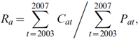
where Ra represents the rate for age group a, Cat the number of cases for age group a in year t, and Pat the population size for age group a in year t.
2.2.1.1.4 Relative percent adjustment method - regional projections derived from scaling down national-level projections (SD)
For a cancer site in a region with average annual counts over the last observed 5 years of fewer than 10, the age-specific counts were also calculated by adjusting the national estimates (based on a modified method used in the Cancer Registry of Norway).Endnote 35 Let w denote the relative difference of the averages of the ASIRs in the last 5 observation years between the region and the whole country, that is,
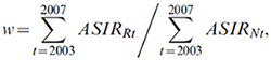
then the cancer incidence rate in a region R, age group a and period p,
RRap = RNap * w = (CNap / PNap) * w,
where RNap, CNap and PNap are the national cancer incidence rate, count and population size at age group a and period p, respectively. For example, if the region had 5% lower rates than the national average in the last 5 observation years, the age-specific rates in each future period were adjusted down by 5% for that region. We therefore have the corresponding number of new cancer cases,
CRap = RRap * PRap.
2.2.1.1.5 Age-specific trend power-5 model fitting single-year data for short-term projections of prostate cancer (ADa)
Trends in prostate cancer incidence since the early 1990s have been subject to overdiagnosis (the detection of latent cancer that would never have been diagnosed in the absence of screening) because of the rapid dissemination of the PSA test.Endnote 36 The projections of period analysis fromNordpred seem unlikely. Therefore, an age-specific trend power-5 model based on yearly data was fitted to a minimum of 8 years of observations from 1994 to 2007 for projections of prostate cancer incidence in the first 5 (2008-2012) or 10 (2008-2017) future years: Rap = (Aa + Da.p)5, where Da is the slope parameter in age group a, which takes the differentiation in trend from different age groups into consideration. This model also allowed for the "spike" value in the year 2001. Another peak year was in 1993, which was excluded from the modelling.
2.2.1.2 Comparison of models
We fitted the projection models described above to observed incidence counts in 1972-1991 and used them to estimate average annual number of cancer cases for the 5-year periods in 1992-2011. Projections were made for males and females, by age group, for the Canadian provinces and at the national level, for the cancer types shown in Table 2.1. Quebec was excluded from this analysis because of data quality issues prior to 1983.Endnote 37, Endnote 38
Given that prostate cancer accounts for nearly one-third of all new cancer cases in males in Canada, the effect of PSA screening is also clearly seen in the incidence of "all cancers combined" in males. The model comparisonswere therefore considered with and without prostate cancer and "all cancers combined" for males when appropriate.
We compared projected average annual numbers of cancer cases with observed values. Median absolute relative difference between projected and observed values, |projected-observed|/observed, was calculated to examine each model's overall tendency to over- or underestimate the actual number of cancer cases. The absolute difference was used when comparing for rare cancers. We compared median prediction errors for each model for combinations of cancer type, geographical area and sex by length of projection. The comparisons considered only combinations for which the models produced projections. We used Friedman's testEndnote 39 to test for statistical difference in medians between different projection models. In addition to considering prediction error across all cancers, we separately compared model performance for each cancer type, across the geographical areas and sexes.
2.2.1.3 Projection validation and adjustment
The model selection was performed by assessing the models and integrating these model comparison results with those from other published studies. However, a model created on cohorts in early periods may give inaccurate predictions when applied to contemporary cohorts. Owing to limitations in the availability of different long-term datasets used for validating the selected models, we examined the projections from the selected models using our knowledge of data quality, trends in cancer rates in different regions, risk factors or interventions to ensure the estimates are appropriate. When the estimated trends seemed unlikely, we used such knowledge to adjust the extrapolation methods of the fitted models, or used Bayesian simulations instead of the generalized linear models. Such modifications were applied in the following situations: all cancers combined in males in Prince Edward Island, Saskatchewan and Alberta, and in females in Ontario, Manitoba and Alberta; female non-Hodgkin lymphoma in New Brunswick; multiple myeloma in males in the Atlantic region and New Brunswick, and in females in Ontario and British Columbia; and thyroid cancer in the provinces except Manitoba, Saskatchewan and British Columbia.
2.2.1.4 Selected models by cancer category
We used the following projection methods in this monograph.
- Common cancers (average annual count over the latest 5 observation years for a national or regional series, N > 50): NP_ADPC model with varied "recent" and "drift" values. One exception is that B_APC was applied to multiple myeloma in males in the Atlantic region as the projections from NP_ADPC seem questionable.
- Less common cancers (10 < N ≤ 50): NP_ADPC or NP_ADP model (based on the significance of the cohort effect and comparison with AVG results) with varied "recent" and "drift" values. The simple age-effect only AVG model has been proven to be the best approach for rare cancers in our model evaluation and other studiesEndnote 27 and has been used in recent reports.Endnote 35 With this, we adopted either NP_ADPC or NP_ADP, from which the projections were closer to the AVG results, instead of basing them solely on linear extrapolation of the 5-year average rate into the future. One exception is that B_APC was applied to multiple myeloma in males in New Brunswick.
- Rare cancers (N ≤ 10): NP_ADPC, NP_ADP, B_APC, B_AP or SD model, whichever projections were closer to the AVG results.
- Prostate cancer: ADa + AVG, defined as
- using ADa to project for the first 5 future years, and then
- using the age-specific average rates of the predicted 5-year data to estimate counts for the second to fifth 5-year periods.
- "All cancers" for males: The estimates of incidence counts were computed as the sum of the estimates for prostate cancer and for all cancers excluding prostate, as estimated by NP_ADPC modelling.
Tables 2.3 shows the selected projection models for rare cancers or in small areas by cancer type, sex and geographical area.
| Cause | Model | |||
|---|---|---|---|---|
| B_APTable 2.3 - Footnote a | B_APCTable 2.3 - Footnote a | SDTable 2.3 - Footnote a | NP_ADPTable 2.3 - Footnote a | |
| Oral | PE/F, TC/M+F | MB/F | ||
| Esophagus | TC/M, NL/F | PE+TC/F | NS/F | |
| Stomach | PE/M | TC/F | PE/F, TC/M | NB/F |
| Colorectal | PE/F | TC/M+F | ||
| Liver | NS/F, TC/M | PE+NL/M+F, NB+SK+TC/F | MB+SK/M, AT/M+F | |
| Pancreas | TC/M+F | PE/M+F | NL/F | |
| Larynx | PE/F, TC/M | PE/M, NS+NB+MB+SK/F | NL+TC/F | AT/F |
| Melanoma | TC/M+F | |||
| Breast | TC/F | |||
| Cervix | PE/F, TC/F | MB/F | ||
| Body of uterus | TC/F | |||
| Ovary | TC/F | PE/F | ||
| Testis | PE+NL+TC/M | NS+NB+MB/M | ||
| Kidney | PE/F | TC/F | TC/M | PE/M, NL/M+F |
| Bladder | PE+TC/F, TC/M | NL/F | ||
| Central nervous system | PE+TC/M+F | NS/M, NB+NL+SK/F, MB/M+F | ||
| Thyroid | PE/M | PE/F | TC/M+F | NS/M, SK/F |
| Hodgkin lymphoma | NB/F | PE+NL+TC/M+F | NB+AB+AT/M, BC/F, NS+MB+SK/M+F | |
| Non-Hodgkin lymphoma | PE/F, TC/M+F | PE/M | NL/M+F, AT+NS+NB/F | |
| Multiple myeloma | AT+NB/M, PE/F | PE/M, NL/F, TC/M+F | NS+MB+SK/M+F, NL/M | |
| Leukemia | PE/M, TC/F | PE/F | TC/M | NL/M+F |
| All other cancers | PE/F | TC/F | ||
|
Abbreviations: AB, Alberta; AT, All Atlantic provinces together (PE, NS, NB and NL); BC, British Columbia; MB, Manitoba; NB, New Brunswick; NL, Newfoundland and Labrador; NS, Nova Scotia; PE, Prince Edward Island; SK, Saskatchewan; TC, All Territories (Yukon, Northwest Territories and Nunavut). Note: The abbreviation before '/' refers to the province or region; 'M' or 'F' after '/' refers to males or females. For example, PE+TC/M+F in the 'SD' model was used for both males and females in PE and TC for central nervous system cancers.
|
||||
2.2.2 Other analysis methods
2.2.2.1 Joinpoint regression analysis
We assessed observed trends (1986-2007) using joinpoint regression,Endnote 40, Endnote 41 which involves fitting a series of joined straight lines on a logarithmic scale to the trends in ASIRs. The trends in incidence are reflected by the annual percent change. The models incorporated estimated standard errors of the ASIRs. The tests of significance used a Monte Carlo Permutation method. The estimated slope from this model was then transformed back to represent an annual percentage increase or decrease in the rate.
A minimum of 5 years of data before and after a changepoint in years in which the annual percent change changed significantly was required for a new trend to be identified. Thus, the most recent possible changepoint is 2003. In Figures 3.1 and 3.2, if no change point was detected from 1998 to 2007, then the annual percent change was estimated by fitting a model within this time period. If a changepoint was detected within this decade, then the annual percent change was estimated from the trend in the last segment. Both the changepoint year and the annual percent change for the years beyond the changepoint are indicated in these two figures.
2.2.2.2 Contribution of change in cancer risk, population growth and population age structure to incidence trend
Figure 3.4 shows the relative contributions of changes in the total numbers of new cases that can be attributed to changes in cancer risk, population growth, and aging of the population. The series were defined as follows (the annual ASIR was calculated by using the average annual population distribution in 1983-1987 for males or females as the standard weights):Endnote 1
- The baseline (red reference line) represents the observed average annual number of new cancer cases during 1983-1987 for males or females.
- The lowest black line represents the average annual number of new cancer cases that would have occurred in each period if the average annual population size and composition had remained the same as they were in 1983-1987. Thus, it measures the impact of changes in cancer risk. This series was computed by multiplying the average annual population in 1983-1987 by the ASIR.
- The middle black line represents the average annual number of new cases that would have occurred if the age distribution of the average annual population had remained the same as it was in 1983-1987, measuring the impact of changes in risk and population growth. This series was computed bymultiplying the average annual population by the ASIR.
- The top line represents the total average annual number of new cases that actually occurred (projected estimates as of 2008) in each period for males or females, reflecting the combined impact of changes in cancer risk, and population growing and aging.
2.3 Presentation of results
In this monograph, while the figures display longer-term time trends in ASIRs of each cancer for broader areas, the tables show cancer incidence frequencies and rates in all provinces and territories from the last observation period (2003-2007) onward. The numbers of cases shown in the tables and figures are average annualnumbers. All the ASIRs were calculated per 100 000 person-years.
For each type of cancer, the historical and projected ASIRs are shown in figures to illustrate their time trends and differences between
- sexes and age groups (<45, 45- 54, 55-64, 65-74, 75-84, 85+), and
- regions (British Columbia, the Prairies, Ontario, Quebec, the Atlantic region and Canada as a whole).
The trends for the North are not shown in the figures because of small numbers. Number of cases in Figure 3.8-3.10 was rounded to the nearest 100.
Tables for males and females give the observed (2003-2007) and projected average annual number of cases and ASIRs by the 10-year age group and province/territories combined. Number of cases was rounded to the nearest 5. The numbers were rounded separately, so it is possible that the totals in the tables do not add up.
Chapter 3 presents the overview of historical and projected trends for all cancers combined, whereas Chapter 4 breaks down such information by cancer sites.
The cancers are ordered by the ICD-O-3 codes.