
Airtightness Measurement of Display Cases and Other Enclosures – Technical Bulletin 38
Jean Tétreault and Eric Hagan
CCI Technical Bulletins
Technical Bulletins are published at intervals by the Canadian Conservation Institute (CCI) in Ottawa as a means of disseminating information on current techniques and principles of conservation of use to curators and conservators of Canada’s cultural objects and collection care professionals worldwide. The authors welcome comments.
Abstract
The purpose of this Technical Bulletin is to explain the advantages of airtight enclosures for the display and storage of heritage collections and to outline a methodology for assessing their performance. Well-sealed enclosures produce tighter environmental tolerances, which can often enhance the preservation of vulnerable objects at a moderate cost. They provide a very effective and sustainable solution for the improved control of agents of deterioration, such as relative humidity (RH) and dust infiltration. A high level of airtightness will reduce inward and outward air movement through leakage points and limit gas diffusion through the enclosure envelope. This performance characteristic is often measured as the rate of loss of a tracer gas, most commonly carbon dioxide (CO2), from an enclosure. Over the past decade, CO2 monitoring data-loggers have become more affordable and easier to use for this task. As a result, determining the airtightness of display cases and other enclosures has become increasingly accessible for the heritage community.
Detailed protocols are provided in this Bulletin for evaluating airtightness and for detecting points of leakage. The guidelines are useful for assessing the performance of existing enclosures and for understanding what to ask for, or expect, during the procurement of products such as display cases. In addition, several case studies present valuable perspectives regarding the use of airtightness values and the justification of the described protocols as well as various limitations and precautions. For example, a high level of airtightness may not always be appropriate for the preservation of objects, especially when sources of agents of deterioration are present or generated within the enclosure.
Authors
Jean Tétreault studied at the University of Montréal, where he received a Master’s degree in Analytical Chemistry in 1989. That same year he joined CCI, where he currently works as a senior conservation scientist in the Preventive Conservation Division. His main research interests focus on pollutants, products used for display and storage, paper degradation and passive environmental controls in collections. Results of his research have been published in various peer-reviewed journals. He has given more than 100 seminars in Canada and Western Europe on preventive conservation issues such as lighting, environmental guidelines, and exhibit and storage materials. Jean is the author of Airborne Pollutants in Museums, Galleries, and Archives: Risk Assessment, Control Strategies, and Preservation Management, a book published by CCI in 2003. He has also published Technical Bulletins on coatings, on products used in conservation and on silica gel. Since 1998, he has been a board member of the Indoor Air Pollution Working Group, which holds conferences every two years.
Eric Hagan holds Master's degrees in Mechanical Engineering and Art Conservation from Queen’s University in Kingston, Ontario. He continued his postgraduate research at Imperial College London with a fellowship from Tate, and he received a Ph.D. in Mechanical Engineering in 2009, studying the mechanical properties of artists’ acrylic paints. He has since worked at CCI, where he is a senior conservation scientist in the Preventive Conservation Division. His recent research activities involve studying the time-dependent mechanical behaviour of artist painting materials, damage analysis of wooden structures with acoustic emission testing and lightfastness experiments on early synthetic dyes. Eric also provides engineering design solutions to Canadian heritage institutions, which include counterbalancing mounts for the Books of Remembrance at Parliament and a low-oxygen capable case for the Proclamation of the Constitution Act, 1982. More recently, he has studied the energy consumption of heritage facilities in relation to local climate and applied tools for performance analysis and benchmarking.
Disclaimer: The information provided here is based on the current understanding of the issues presented. The guidelines given in this Technical Bulletin will not necessarily provide complete protection in all situations or protection against every possible adverse effect caused by incorrect RH, incorrect temperature and unacceptable levels of pollutants in museum contexts. CCI does not provide any guarantee with respect to any person or institution that uses the airtightness determination protocol described in this Technical Bulletin. CCI also assumes no responsibility for consequences resulting from use of the information contained herein.
Table of contents
- List of abbreviations
- Introduction
- Agents of deterioration
- Detecting points of leakage
- Determination of airtightness with the tracer gas method
- Protocol
- Methods for calculating the airtightness
- Airtightness as a specification
- Case studies
- Case study 1: specify an airtightness based on silica gel maintenance
- Case study 2: risk of lead corrosion in a display case made of oak
- Case study 3: the effect of temperature on equilibrium CO2 content
- Case study 4: the effect of a fan
- Case study 5: justification for the test duration
- Case study 6: multiple compartment display case
- Case study 7: error and reproducibility
- Acknowledgements
- Appendix A: Airtightness checklist
- Appendix B: Graham’s law of diffusion
- Bibliography
List of abbreviations
- AER
- air exchange rate (unit: 1/day or day-1)
- AIC
- American Institute for Conservation
- BSI
- British Standards Institution
- CCI
- Canadian Conservation Institute
- IEC
- International Electrotechnical Commission
- ISO
- International Organization for Standardization
- MDF
- medium-density fibreboard
- N
- airtightness (unit: 1/day or day-1)
- NPS
- National Park Service
- ppb
- part per billion (by volume)
- ppm
- part per million (by volume)
- R2
- coefficient of multiple determination
- RH
- relative humidity
- RSD
- relative standard deviation
- SD
- standard deviation
Introduction
An enclosure is a structure that surrounds a specific volume of space, in which one or more objects are contained for protection against the different agents of deterioration. Examples include display cases, storage cabinets, boxes, plastic bags and shipping crates. Airtightness is one of the primary concerns for safeguarding against exterior agents such as gaseous pollutants, dust, insects and RH. An accurate measure of this parameter helps to predict the conditions of the environment inside the enclosure and the degree of protection provided to objects.
Heritage institutions are increasingly requesting enclosures with specific airtightness levels, particularly for display cases, and they are requiring proof of their performance. At the same time, environmental monitors have become more common and affordable for the museum community. This allows museum staff to check for themselves if improvements are needed and also to confirm if new display cases meet the predefined airtightness specifications.
The aim of this Technical Bulletin is to provide an overview of the advantages of airtight enclosures for the display and storage of heritage collections and to outline a methodology for assessing their performance. The Bulletin contains descriptions of the common approaches for measuring airtightness, tools for locating points of leakage and clear examples of the influencing factors. Focus is given to the method of quantifying airtightness from the decay of carbon dioxide (CO2) tracer gas, which is used to calculate the air exchange rate (AER).
Leakage mechanisms
Typical leakage mechanisms are broadly divided into two categories:
- airflow (carrying gas or small particles) in and out of the enclosure due to air pressure differentials; and
- diffusion of gases into and out of the enclosure through construction materials or through still air in gaps, holes or seams.
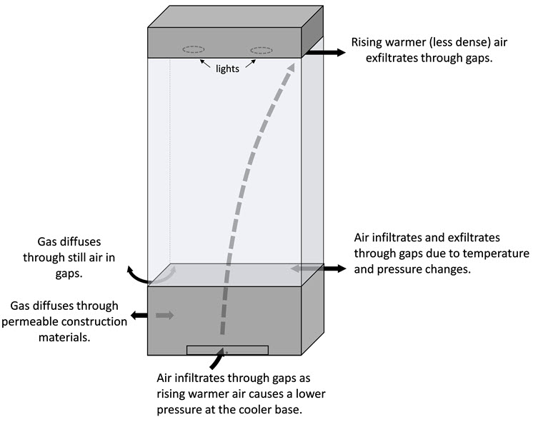
These processes are illustrated for a display case in Figure 1.
© Government of Canada, Canadian Conservation Institute. 132731-0001
Figure 1. Illustration of typical leakage mechanisms for display cases: vapour, gas or dust transport by airflow through gaps and gas diffusion through construction materials or still air in small gaps. A theoretical display case is shown, consisting of a wooden base with sorbent access, glass glazing and an overhead lighting cabinet.
The first process, involving airflow, may result from changes in atmospheric pressure that cause the pressure inside the enclosure to be lower or higher than that which is in the room environment. This leads to forces that pump air into and out of the enclosure through gaps, carrying with it gases or small particles (such as water vapour, pollutants or dust).
A small pressure differential may also occur if the temperature inside the case is different from that of the room. For example, the temperature may increase from lighting during exhibit hours (pushing air out by expansion) and may normalize during off-hours (drawing air back in). Similarly, diurnal cycling of the room temperature may result in a pressure differential between the enclosure and the room.
A temperature gradient within a display case may also cause airflow leakage through its effect on air density and air pressure. This is commonly called the “stack” or “chimney effect,” and it may occur in taller enclosures where the less dense warm air rises and causes a lower pressure at the base. The lower pressure pulls cooler air in through gaps around the base area, while warmer air leaves through gaps around the top. Humidity is also a factor in this leakage mechanism, since moist air is more buoyant (less dense).
The second process involving diffusion of gases through still air and construction materials is generally slower, especially through solids. The rate of transfer through construction materials depends on the type and thickness of the solid material, the type of penetrating gas and also the concentration gradient across the envelope. The diffusivity of a particular gas through the material is expressed as a diffusion coefficient, which is experimentally determined from standard test methods. It is beyond the scope of this document to fully review the mathematics and physics of permeability and diffusion; however, some published diffusion coefficients for water vapour transmission through common construction materials are presented after conversion to similar units and scale (m2/s × 10-12).
- Acrylic [poly(methyl methacrylate)], 0.12 to 0.21 mm membrane: 1.1 to 1.8 and higher as reviewed by Roussis (1983) and described as more complex than simple diffusion due to polymer relaxation over large time scales.
- Plywood, 25 mm beech: 51.6 (Sonderegger 2009)
- Medium-density fibreboard (MDF), 25 mm: 283 (Sonderegger 2009)
- Melamine-faced MDF, 25 mm: 44.7 (Sonderegger 2009)
It is clear from the list above that uncoated wood products transport water vapour much faster than acrylic glazing at a given thickness. For diffusion coefficients as a function of wood species, grain direction, moisture content and even tree section (sapwood versus heartwood), consult Choong (1968). Note that the addition of coatings can also influence the overall transfer of water vapour, and it will vary significantly by product (Yaseen 1978).
In summary, the leakage of an enclosure is often a complex scenario involving a mixture of mechanisms, and an airtightness test is used to quantify and analyze the net effect. For further information regarding these leakage processes, consult Padfield (1966) and Michalski (1994).
Airtightness
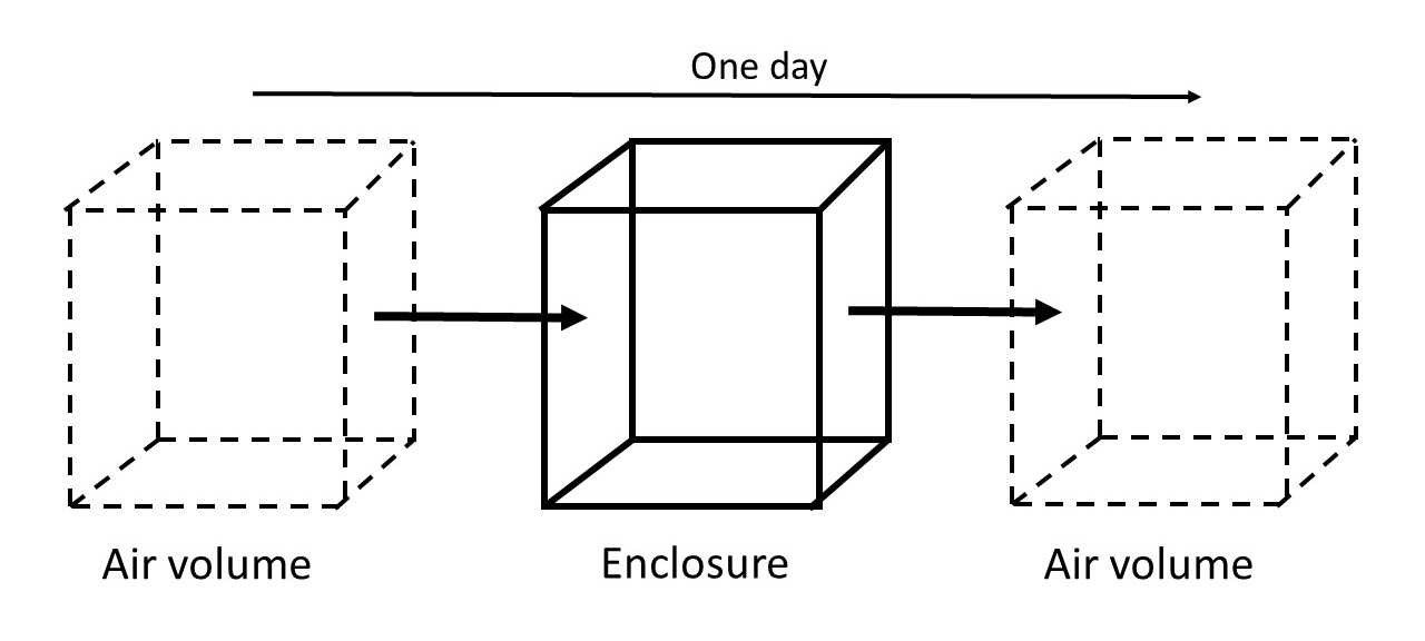
In the context of this Bulletin, airtightness is the resistance to gas transfer through holes or gaps and by diffusion through the enclosure envelope. To quantify this, the airtightness (N) or AER is defined as the number of times that air is replaced in an enclosure every hour or day, with units of 1/hour (hr-1) or 1/day (day-1), respectively. The value is typically determined by measuring the decay of a tracer gas from an enclosure, and it is expressed in terms of days, since the leakage is usually quite slow. An airtightness of one per day means that one volume of external air enters in a day and that one volume of air leaves (Figure 2).
© Government of Canada, Canadian Conservation Institute. 132731-0003
Figure 2. Schematic illustration of one air exchange per day. The air volume equivalent to the enclosure volume is entering and leaving the enclosure every day.
Another way to express the airtightness is in terms of one air exchange every X number of days. For example, you may have one air exchange every two days, which is similar to 0.5/day. Leakage rate, air changes per day and number of changes of air volumes per day are synonyms of airtightness. Confusion may exist in the varied terminology. An improvement in airtightness refers to a lower AER and vice versa. In general, the term “airtightness” is used throughout this text. However, when there is reference to the notion of an increasing or decreasing rate, the term "AER" is used instead.
Tracer gas
A tracer gas is a gas used for the determination of leakage points or for the quantification of the airtightness of enclosures. The tracer gas must be safe for humans in the concentrations used for the application. Ideally, it will not interact with objects and enclosure materials or become adsorbed. Its presence in the local environment should be very small compared to the concentration used for the test.
Tracer gases used in the museum context include carbon dioxide (CO2), nitrous oxide (N2O), fluorocarbon (PFT), sulfur hexafluoride (SF6), helium (He) and hydrogen (H2). Refer to the safety material sheet (SDS) of the gas canister used, especially if amounts larger than the typical application are required. The gas detection instrument should be easily accessible and easy to operate, and it should have a fast measurement response.
With respect to climate change, CO2 is a greenhouse gas and typically a by-product of petroleum extraction. CO2 has a global warming potential of 1 (reference value), while the impact for N2O and SF6 is much worse, with a potential of 298 and 22,800, respectively (Solomon et al. 2007). In practice, using CO2 in the context of airtightness measurement has little impact on climate change since the average person releases about 900 g of CO2 in a day (LeMone 2008) and a 1 m3 enclosure filled with 5000 ppm contains only 9 g of CO2.
Water vapour is occasionally used for the determination of airtightness. While it can give an estimate of the enclosure’s airtightness, results are strongly influenced by the moisture sorption of hygroscopic materials inside (Daniel and Maekawa 1992; Calver et al. 2005).
In some special enclosures, such as an anoxic (without oxygen) case, oxygen or helium are used as tracer gases (Smith et al. 2016; Robinson 2011). The enclosure is flushed with nitrogen or helium and then sealed. The monitor records if the tracer gas level is increasing (oxygen ingress) or decreasing (helium egress).
An air pressure test with a manometer can also be used for the determination of airtightness; however, it is much less common. The manometer is used to monitor the decay of initially supplied pressure as air leaks from the enclosure and normalizes with the room environment. It is important to test at both increased and decreased pressure, as compression seals act differently in the two instances. Some information regarding this technique is provided by Perino (2018).
Agents of deterioration
There are many advantages to very airtight enclosures. They can block or, at least, reduce the impacts of different agents of deterioration. They can also maintain an adequate environment at a low cost if the environment control in the room is insufficient. However, in some contexts, very airtight cases may cause adverse effects. The impacts of the airtightness on some agents of deterioration are reviewed in this section.
Relative humidity
Occasionally, it is more convenient to passively control RH in one or more enclosures rather than the overall room. Passive control of RH is typically accomplished with a moisture sorbent such as silica gel. An airtight enclosure allows for the optimization of RH control with minimal effort, since it requires less sorbent and less frequent sorbent regeneration to maintain target levels. Internal RH control is used to minimize RH fluctuations or to maintain a specific RH in the enclosure that is lower or higher than the RH in the room.
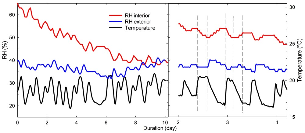
For example, Figure 3 describes an RH and temperature trend inside and outside a display case having an airtightness of 0.44/day. On the left is the trend during the period of March 1 to 11, 2021, without a moisture sorbent. It takes about nine days for the interior RH to reach the RH in the room. It will take less time if the case is leakier. On the right is the trend at a narrow day range: as the external temperature fluctuates, the RH in the room fluctuates in the opposite direction with some delay, as does the RH in the case with a slightly longer delay. A fluctuation cycle is well observed between the fourth and fifth day. For the same period, curves in the graphs may look different since the sampling rate is different. The rate is every 3 hours on the left and every 30 minutes on the right.
Active RH control systems for enclosures also exist and work best with relatively well-sealed cases.
© Government of Canada, Canadian Conservation Institute. 132731-0005
Figure 3. An RH and temperature trend inside and outside a display case having an airtightness of 0.44/day.
Equation 1 shows the relationship between the quantity of moisture sorbent needed to control the RH in the enclosure with respect to airtightness and several other parameters. The equation has been verified by Thickett et al. (2007) and Thickett (2018). Detailed information on the use of this equation can be found in Technical Bulletin 33 Silica Gel: Passive Control of Relative Humidity.
Equation 1:
Where
Q = quantity of dry sorbent recommended (kg)
Ceq = concentration of water vapour at equilibrium (g/m3)
D = decimal difference between the RH outside the enclosure and the targeted RH inside (no unit)
V = net volume of air in the enclosure (m3)
N = airtightness (1/day)
tmin = minimum number of days the targeted RH range must be maintained (days)
MH = specific moisture reservoir of sorbent, including the effect of hysteresis (g/kg for a 1% RH change)
F = targeted range of RH fluctuation (%)
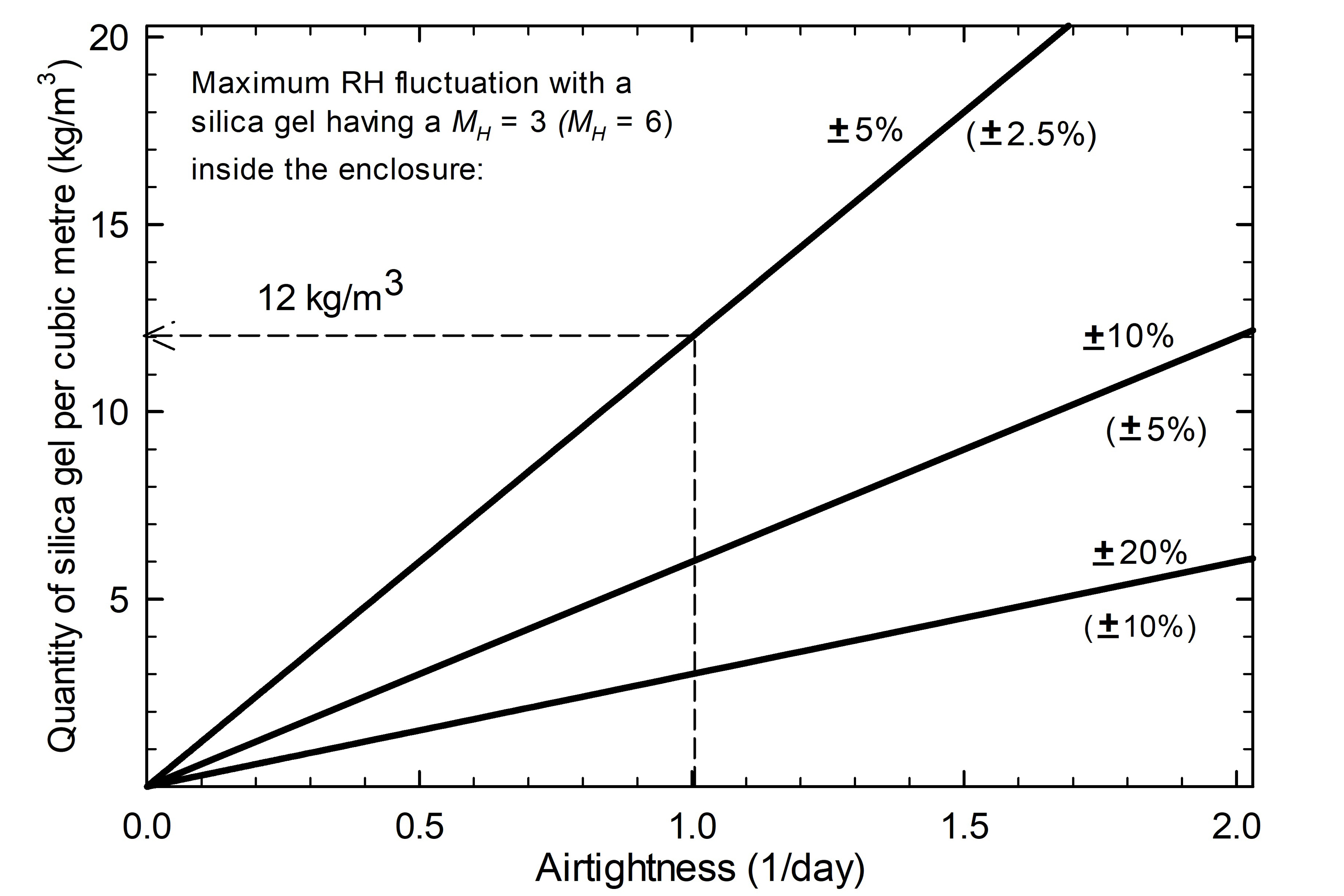
Figure 4 illustrates an example of the relationship between the quantity of moisture sorbent and the airtightness. It is evident that highly airtight display cases require less moisture sorbent to maintain the desired RH range and that the sorbent requires reconditioning less often.
© Government of Canada, Canadian Conservation Institute. 132731-0007
Figure 4. Amount of silica gel required to maintain stable RH conditions over an annual cycle according to Equation 1. The three diagonal lines represent different acceptable ranges of humidity fluctuation within the display case.
Description of Figure 4
The graph shows the relationship between the quantity of moisture sorbent [the y-axis is quantity of silica gel per cubic metre (kg/m3)] and the airtightness with different target RH fluctuations. The x-axis is an airtightness of 1/day. If the silica gel has a specific moisture reservoir of 3 g/kg for a 1% RH change, the enclosure will need 1.12 kg/m3 to maintain RH fluctuations within ±5%; 2.6 kg/m3 to maintain RH fluctuations within ±10%; 3.3 kg/m3 to maintain RH fluctuations within ±20%. With silica gel having a specific moisture reservoir of 6 g/kg for a 1% RH change, all of the RH fluctuations are halved.
Trends shown in Figure 4 were derived with the following assumptions:
- the enclosure contains regular (type A) silica gel with MH = 3 (values in parentheses are based on high performance silica gel with MH = 6);
- the RH outside the enclosure is in the range of 30% to 70% with a maximum fluctuation of ±20%; and
- the RH within the enclosure is maintained at 50% within a range of F.
The graph shows that with an airtightness of 1.0/day, the quantity of sorbent needed is 12 kg/m3 if the maximum RH fluctuation allowed is ±5%. With an AER reduced to 0.5/day, only 6 kg/m3 is needed.
An unwanted high RH in airtight enclosures is possible in certain circumstances. This may occur as a microenvironment (for example, via temperature gradient), which can be favourable to mould growth and chemical reactions. The following four precautions will help to prevent this scenario:
- Avoid temperature fluctuations of more than 5°C in the room.
- Avoid the contact of the enclosure with a cold wall.
- Avoid storing damp objects in the enclosure.
- Avoid placing objects in the enclosure during damp periods (≥ 75% RH).
Examples of the use of airtightness to optimize the performance of silica gels are outlined in Case study 1: specify an airtightness based on silica gel maintenance.
Airborne pollutants
The airtightness of enclosures may be an advantage or a disadvantage for controlling gaseous and particulate pollutants, depending mainly on where the source is located. Outdoor pollutants and pollutants generated in the building from materials or human activities can infiltrate enclosures. Airtight enclosures can block or, at least, reduce this infiltration.
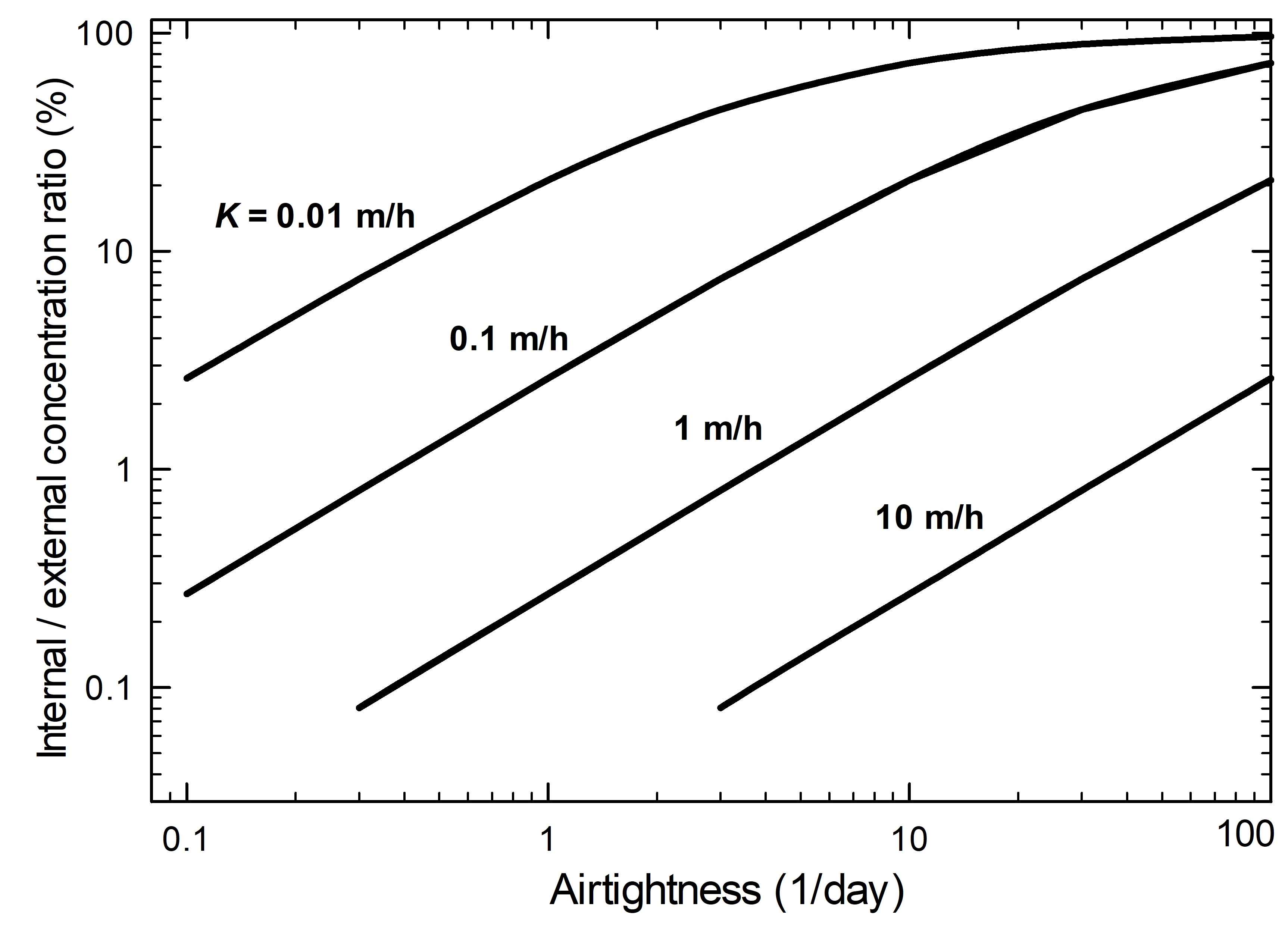
Equation 2 defines how the airtightness influences the ratio of inside and outside concentrations of a gas (Weschler et al. 1989). This relationship is also illustrated graphically in Figure 5. Note that the equation excludes the internal generation of pollutants.
Equation 2:
Where
Cin = internal concentration (µg/m3)
Cex = external concentration (µg/m3)
K = mass transfer coefficient (absorption) (m/h)
N = airtightness (1/day)
S = surface area of the material (m2)
V = net volume of air in the enclosure (m3)
© Government of Canada, Canadian Conservation Institute. 132731-0009
Figure 5. Ratio of internal concentration to external concentration of a volatile compound as a function of enclosure airtightness and different mass transfer coefficients (K).
Description of Figure 5
The graph shows the relationship between the internal and external concentration ratio (y-axis) and the airtightness of the display case (x-axis is an airtightness of 1/day) having materials with different mass transfer coefficients (absorption). For a specific mass transfer coefficient, a reduction of the airtightness value gives a smaller concentration ratio. Further reductions of the ratio occur with smaller loads.
As the AER decreases (airtightness improves), the ratio of internal concentration to external concentration decreases. Less infiltration is then possible, which results in a lower internal concentration. The absorptivity of materials in the enclosure, also referred to as the mass transfer coefficient or deposition velocity, affects the indoor concentration. The higher the absorptivity, the lower the inside concentration. Deposition velocities for different pollutant-material systems are compiled in Tétreault (2003, p. 136).
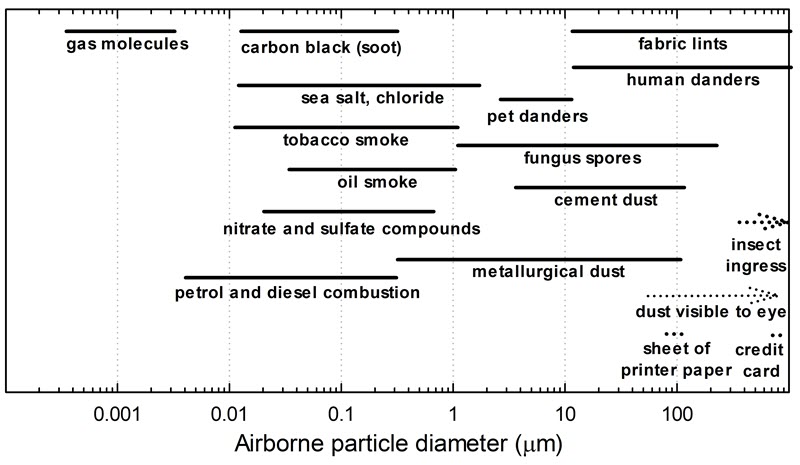
The dust deposition in an enclosure is also dependent on airtightness. Dust can be composed of various compounds, from tiny particles of combusted materials to heavy fabric lint or human dander, as shown in Figure 6. Based on experimental data from Thickett (2018), the internal and external dust deposition ratio in percent (%) is directly proportional to airtightness: AER (1/day) multiplied by a factor of 24. This relation is valid for dust having an aerodynamic diameter of 20 to 200 µm in the airtightness range of 0 to 2 per day with a standard deviation (SD) of 20%. An enclosure with an AER of 1/day has an internal and external coarse dust deposition ratio of 24%, which means that the deposition rate inside the enclosure is about four times slower than outside. This factor represents the reduction of mainly large dust particles such as those generated by humans from clothing, pet dander, some fungus spores and cement dust. The infiltration of dust having a diameter much smaller than 20 µm should act more like a gas. Particles greater than 200 µm have a short suspension time and can infiltrate an enclosure only if generated in close proximity in busy galleries.
© Government of Canada, Canadian Conservation Institute. 132731-0011
Figure 6. Dust distribution. The thickness of a credit card and a standard sheet of printer paper are shown as references.
Description of Figure 6
The graph shows the comparative size of various pollutants in particle sizes between 0.0001 and 1000 µm. The size for gas molecules is the smallest, between 0.0003 and 0.003 µm. Petrol and diesel combustion molecules range in size from 0.003 to 0.3 µm. Carbon black (soot) particulates range from 0.01 to 0.5 µm. Tobacco smoke particulates range from 0.01 to 1 µm. Sea salt, chloride particles range from 0.01 to 2 µm. Nitrate and sulfate compounds range from 0.02 to 0.7 µm. Oil smoke particulates range from 0.03 to 1 µm. Metallurgical dust ranges from 0.5 to 100 µm. Fungus spores range from 1 to 200 µm. Pet danders range from 2 to 10 µm. Cement dust ranges from 3 to 100 µm. Fabric lints and human danders have the same range for particle sizes: from 10 to 1000 µm. Dust visible to the eye ranges between 50 µm and up. The thickness of a credit card is 760 µm, and a standard sheet of printer paper is 70 to 100 µm. Insect ingress is 330 µm and higher.
In the past, focus was given to preventing infiltration of outdoor or indoor pollutants in enclosures. As enclosures such as display cases became more airtight, new problems started to arise due to pollutants generated inside. This happens when concentrations increase due to an emission rate faster than their exfiltration.
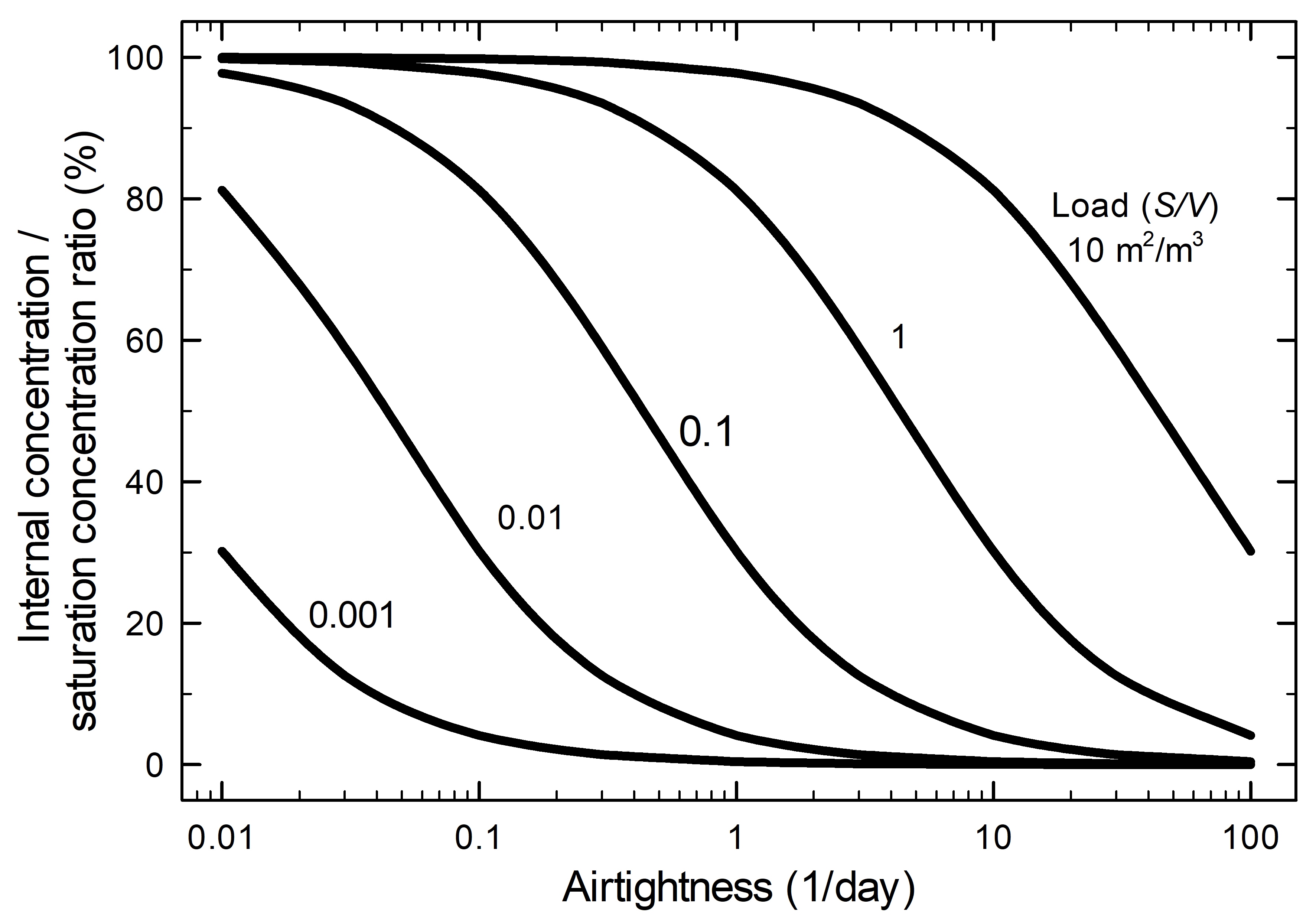
Equation 3 shows how airtightness affects the ratio of the internal concentration to the saturation concentration (Meyer and Hermanns 1985). This relationship is presented in Figure 7.
Equation 3:
Where
Cin = internal concentration (µg/m3)
Csat = saturated internal concentration (µg/m3)
K = mass transfer coefficient (absorption) (m/h)
N = airtightness (1/day)
S = surface area of the material (m2)
V= net volume of air in the enclosure (m3)
© Government of Canada, Canadian Conservation Institute. 132731-0013
Figure 7. Ratio of internal concentration to saturation concentration of a volatile compound emitted by a product inside the enclosure as a function of the airtightness and based on different loads.
Description of Figure 7
The graph shows the relationship between the internal concentration and saturation concentration ratio (y-axis) and the airtightness (x-axis is an airtightness of 1/day) having different loads. For a specific load, an increase of the airtightness value gives a smaller ratio. With smaller loads, further reduction of the ratio will occur.
The scenario used for the graph is based on one volatile compound emitted by a product in the enclosure. The mass transfer coefficient used is 0.18 m/h based on the emission of acetic acid from oak. The saturation concentration is the maximum concentration that a volatile compound can reach in an absolute airtight enclosure without any sorption materials. As the AER decreases, the concentration ratio increases and, consequently, the internal concentration increases as well.
The internal concentration is also influenced by the load of the source. The load is the ratio of the emissive surface to the net volume of the enclosure. For a fixed airtightness, a high mass transfer coefficient (or highly emissive material) pushes the internal concentration toward the saturation concentration. An example of the use of Equation 3 is found in Case study 2: risk of lead corrosion in a display case made of oak.
High concentrations of various gases emitted by enclosure and object materials can be a threat for the objects (including the emissive ones). However, many gases are harmless and some may even give limited protection to objects. Research related to the conservation of flexible poly(vinyl chloride) (PVC) shows how airflow around objects made of this material can affect the plasticizer at the surface (King et al. 2020). Further study is needed to understand the effects of various gases on materials in enclosures. With substantially emissive materials, it is often best to remove problematic materials or to remove sensitive objects from the enclosure. Otherwise, the enclosure should be modified to increase natural exfiltration or provide active ventilation. It is best to choose materials that are generally accepted in conservation or tested to confirm their low reactivity (Tétreault 2017).
In applications strictly concerning pollutants, the optimal level of airtightness requires consideration of the impacts of the infiltrated pollutants as well as those generated inside the enclosure. Equation 3, when combined with knowledge of an enclosure’s airtightness, will help to predict the level of pollutants in that enclosure. Information on the risk posed by those pollutant levels on different objects can be found in Tétreault (2003, pp. 106–130) and Tétreault (2021).
In some situations, oxygen is an adverse agent and is classified as a pollutant due to its capacity to cause chemical damage. On rare occasions, a highly airtight enclosure is specified (for example, in the preservation of very significant objects or objects that are very sensitive to oxygen, such as natural rubber). An anoxic microenvironment prevents their oxidation. Typically, the oxygen is flushed with an inert gas such as nitrogen, and an oxygen absorbent is added to the enclosure (Daniel and Lambert 1993). The performance and the duration of the low-oxygen environment depend on the airtightness and the quantity of absorbent (even if the term “absorbent” is commonly used here, the removal of oxygen is performed by chemical reactions). Typically, great protection is provided by anoxic enclosures; however, there are some materials that can deteriorate faster or differently in anoxic microenvironments. Some exceptions have been quantified by Beltran et al. (2012) with respect to light exposure under low-oxygen conditions.
Fire
A combustible airtight enclosure may offer limited protection against direct fire; however, it can prevent significant damage during a small fire by slowing the infiltration of smoke (consult Airborne pollutants). Heat transfers through glazed enclosures can be an issue (consult Light and temperature). Airtight enclosures will also minimize the impact of water during fire suppression actions.
Light and temperature
Direct sunlight or close bright artificial light sources can generate an undesired elevated temperature in a glazed case due to the greenhouse effect. Many types of materials and objects in display cases can absorb radiation from light sources, especially those with dark surfaces. They can elevate the temperature inside cases by re-emitting radiation at lower wavelengths (especially infrared) and also by conduction. This can be an issue if the light level is high. Leaky cases may be able to dissipate some warm air.
Temperature fluctuations also affect the airtightness (Holmberg and Kippes 2003; Thickett et al. 2005; Watts et al. 2007) by causing a pressure (or air density) differential as well as affecting the sorption capacity of materials in the enclosure, which causes perturbations to the AER. For more information, consult Case study 3: the effect of temperature on equilibrium CO2 content.
Insects
An airtight enclosure prevents insect infiltration. It was reported that a gap below 330 µm protects against insect ingress (Strang 2012, p. 145). If insects are already inside a well-sealed enclosure, they may damage objects; however, their confinement will protect the rest of the collection. A highly airtight case with low oxygen can also be used for the eradication of insects in objects (Maekawa and Kerstin 2003).
Water
A well-sealed enclosure can also prevent water infiltration from the bottom during a flood event, from the top during a water leak incident and from the side in case of a burst pipe or due to possible spilling by vandals or guests during special events. It is recommended to keep enclosures at least 10 cm from the ground. This will avoid most ingress of water due to small floods. Some museums may have interest in enclosures offering protection against dripping water; for example, passing the test of water dripping for 30 minutes (Underwriters Laboratories 2015).
Vandals and theft
The absence of obvious gaps in the display cases may decrease the risk of vandalism or theft.
Detecting points of leakage
A simple visual survey can identify major points of leakage that require sealing for improved case performance. During this process, the use of a piece of paper or credit card (or equivalent) indicates gaps that are relatively simple to fix. The next level of investigation involves locating points of leakage with instrumentation (typically a refrigerant or ultrasonic leak detector). There is an advantage to using both measurement techniques, since one detector may find leakage points that are undetected by the other method. The various methods for leakage assessment are outlined here.
Visual assessment of gaps
In the absence of expensive instruments, it is often straightforward to visually locate sites of suspected leakage. Start by looking closely inside and outside each surface and interface, taking note of the following common areas where leakage occurs:
- interfaces between mated surfaces, such as glazing panels, doors and structural elements;
- around access points, such as the sorbent compartment door;
- gaskets and sealants that are poorly fitted, degraded or missing;
- keyholes;
- through-holes for electrical wires, lighting components or other accessories; and
- loose, distorted or missing fasteners.
Pay particular attention to surfaces that are designed to be opened or disassembled and to areas around accessories (lighting connections, locks, etc.). Surface irregularities and deformation from mechanical reinforcement can cause a gap to form over time. This often occurs in modern display case designs with large glazing panels, which bend outwards in the middle due to clamping forces at the ends. Additional factors can lead to poorly fitted gaskets: improper materials (thickness, compliance, profile type), assembly flaws, case deformations, poor splicing at corners, chemical degradation (aging), compression set or a combination of these issues.
Signs of pests in the enclosure may indicate that there is at least one leakage point large enough for insects to enter. The observation of live or dead insects suggests a crack or gap that is 330 µm or larger (Strang 2012, p. 145). It is also important to keep in mind that insects may come from objects in the display case.
Paper tests
A feeler gauge is valuable for determining a specific gap thickness; however, a simple sheet of paper provides a useful reference for thickness, since the gauge tool is often unavailable. While performing the visual assessment, try sliding the paper into different interfaces of the enclosure, such as between two glass panels. A standard sheet of printer paper (70–100 µm thick) detects gaps of 100 µm or larger. Insects are unable to enter if a sheet of paper cannot pass through, since the gap is less than the ingress threshold of 330 µm. In comparison, the thickness of a credit card is 760 µm (ISO/IEC 7810 2019). A gap of this size would indicate that insect ingress is possible (consult Figure 6 for the typical diameter of different items). Another option to check for possible insect ingress is to use three or four sheets of stacked printer paper or to have materials such as cardstock premeasured with calipers, which can be used to check the size of gaps.
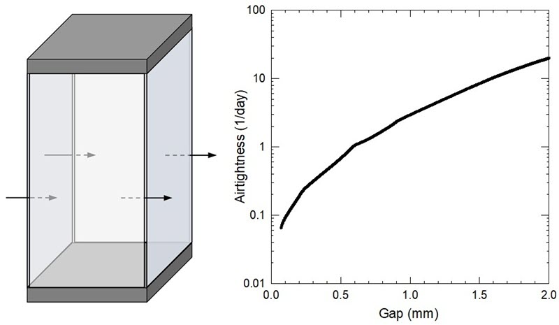
It is possible to predict the airtightness based on gap thickness with a simple enclosure leakage model based on Michalski (2017). Figure 8 shows the effect of gap width between four glass panels of a display case on the corresponding airtightness. Several parameters are used in the model:
- interior volume of 1.28 m3 (80 × 80 × 200 cm);
- uniform gaps along glass panels;
- no other leakage points in the case (difficult to achieve in practice); and
- a daily temperature fluctuation of ±2°C.
In this example, all of the gaps must be smaller than 600 µm to obtain an airtightness below 1/day. If it is not possible to insert a 100 µm sheet of paper through any gaps, the airtightness could be below 0.1/day.
© Government of Canada, Canadian Conservation Institute. 132731-0015
Figure 8. A display case made with four tall glass panels (left), and the effect of gap width between panels on airtightness (right).
Description of Figure 8
An image on the left contains arrows that indicate potential air movement between the four glass panels of a display case. Air moves in as well as out of the case. A graph on the right shows that as the gap between panels becomes smaller (x-axis is the gap in millimetres), the airtightness improves (y-axis is an airtightness of 1/day).
Electronic leak detection
The primary points of leakage are not always easy to identify through a combination of visual assessment and the paper test, particularly when targeting higher levels of airtightness. The next level of investigation involves electronic leak detection techniques, which use a chemical or physical source in the enclosure and an external sensor to locate its egress. The user must scan all surfaces with the detector to find where the tracer gas or ultrasonic signal is leaking out. The detection efficiency depends on the intensity of the source and the sensitivity of the instrument. A leak detector may not locate all leakage points when some areas of the enclosure are hard to access, particularly for inset wall cases.
Tracer gas leak method
The use of a tracer gas and corresponding detector is a rapid method for detecting larger leaks, particularly in open gaps. It is not appropriate for slow leakage processes through very small holes or for diffusion through materials.
Chemical tracer gases are typically perfluorinated compounds used as a refrigerant or propellants in air dusters for electronics. Commercial refrigerant leak detectors detect these gases, and the device is often available in a building operator’s toolkit. Another option is to use a source of 5% H2, since concentrations below 5.7% H2 are non-flammable. For more information, consult the section Tracer gas.
Figure 9 shows the general steps involved in this type of leakage detection:
- injecting tracer gas into the display case,
- waiting a few minutes for dispersion and
- canning areas for leaks with a detector.
There is often limited control in tracer gas delivery, and some experimentation is required to determine the appropriate amount to use for a given case size. It may be necessary to inject gas multiple times due to losses during the time taken for gas to reach leakage points. Removing the display support plate, if this is possible, may accelerate the internal diffusion. Also note that some gas may linger at the injection site; therefore, it is helpful to start scanning in a different area of the case.
© Government of Canada, Canadian Conservation Institute. 132731-0017
Figure 9. Detecting points of leakage with tracer gas.
Ultrasonic method
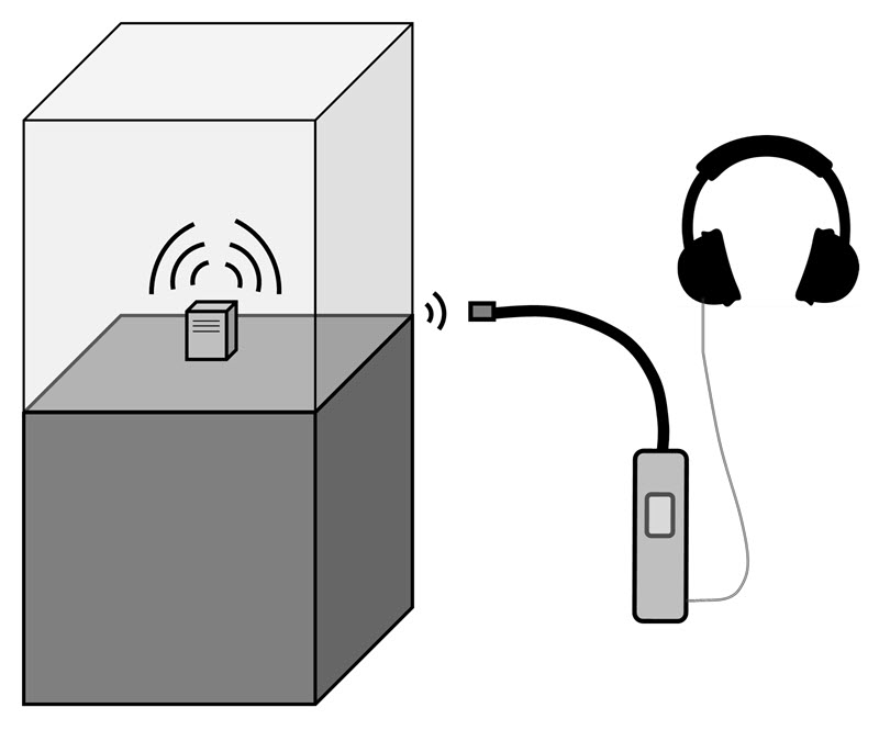
Locating leaks with an ultrasonic emitter and detector is similar in principle to the tracer gas method. Ultrasonic leak detection is used in many fields, and the application most similar to display cases is the location of building envelope leaks. When looking for an instrument, take care to note the difference between an emitter/receiver device versus strictly an ultrasonic detector (for compressed gas leaks).
In our application, an emitter of ultrasonic frequencies centred at about 40 kHz is placed inside the display case. The user scans outer areas with a detector probe that is sensitive to the emitter frequency. Leak detection is observed by an audible signal. A simplified schematic of this setup is illustrated in Figure 10. This is typically a qualitative test for leak identification; however, a general sense of the leakage magnitude is observed by the signal’s intensity.
© Government of Canada, Canadian Conservation Institute. 132731-0018
Figure 10. Detecting points of leakage with the ultrasonic technique.
Determination of airtightness with the tracer gas method
Determination of the airtightness of an enclosure is typically performed with a tracer gas. The equipment needed for the test is the source of the tracer gas, the tracer gas injector and the tracer gas monitoring data-logger. This section covers each of the three aspects.
Carbon dioxide as tracer gas
Carbon dioxide (CO2) is a common tracer gas, and it is easily accessible for the determination of the leakage rate. Indoor background levels tend to be in the range of 400–1000 ppm, depending on the degree of human activity in the vicinity (human breathing generates CO2).
Many health jurisdictions in Canada rely on the American Conference of Governmental Industrial Hygienists to set their own CO2 exposure limits. The eight-hour limit is 5,000 ppm, and a peak allowance is 30,000 ppm (usually for 15 minutes) (Canadian Centre for Occupational Health and Safety 2021). In 2021, Health Canada proposed a CO2 limit of 1000 ppm for daily exposure in its Residential indoor air quality guidelines. The typical use of small, compressed CO2 cartridges for the determination of enclosure airtightness should fall easily into these safe concentration limits.
In terms of the risk of damaging objects, it seems to remain low with CO2. CO2 can be transformed into carbonic acid in water (H2CO3). Injecting CO2 in water will give a pH in the range of 3 to 4. This transformation is easily reversible when the bottle of carbonated water is open. Fortunately, the formation of the acid is not favoured with water vapour in the air. Kigawa et al. (2011) observed slight chemical changes on animal proteins after being exposed to 600,000 ppm of CO2 for two weeks. Thickett (2012, pp. 107–109) mentioned the concern of lead corrosion transforming from basic lead carbonate to lead carbonate in the presence of CO2. To investigate this theory, basic lead carbonate powder was monitored after exposure to 20,000 ppm of CO2 for seven days, and very little change was noticed. As a precaution, it is recommended that a CO2 injection be performed when the ambient RH is below 75%.
While chemical damage is not expected during leakage tests, enclosure materials and the objects themselves have varying capacities to absorb CO2, which can affect the determination of the airtightness. The effect of silica gel, activated carbon, wood and books is investigated in Case study 3: the effect of temperature on equilibrium CO2 content. Activated carbon, specifically, causes an important shift of the CO2 concentration.
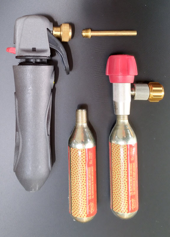
Tracer gas injector
CO2 injector devices are commonly found on the market for uses such as home brewing and bicycle tire inflation (Figure 11). These applications often use 12 g or 16 g cartridges (heavy CO2 users can work with a 2.3 kg cylinder). The small cartridges contain CO2 in a liquid/gas equilibrium with a pressure around 5700 kPa (825 PSI) at room temperature. For this reason, the cylinders are only eligible for ground transportation. The supplied injector kit often contains one CO2 cartridge. Take note if the cartridge is unthreaded or threaded, as this is important to know for future purchases.
© Government of Canada, Canadian Conservation Institute. 132731-0019
Figure 11. Two CO2 injectors compatible with threaded cartridges. One (grey) design for a bike has a custom brass extension tube, and the second design has a mini regulator.
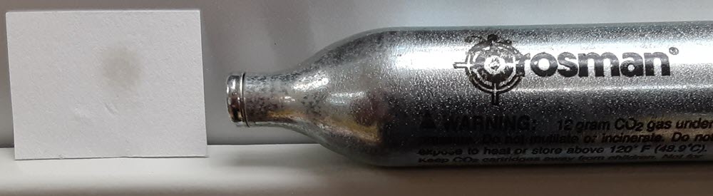
Pure CO2 is odourless; however, its source from combustion or a fossil fuel reservoir is far from clean. Some CO2 supplies are simply not designed for the food market or an unventilated room. For such cartridges, the presence of significant hydrocarbons and oily residues is possible due to minimal filtration during manufacturing.
We can classify the purity of CO2 cartridges in three groups: food grade, filtered and unspecified. In Figure 12, two cartridges of unspecified purity were released on a piece of paper, leaving a stain and generating an unpleasant smell in the vicinity. Filtered cartridges can leave some residue on paper (about 2/3 less than from the unspecified variety), with little or no unpleasant smell. The food grade cartridges are not smelly and do not cause stains. As a precaution, it is best to avoid using CO2 cartridges of unspecified purity to test enclosures containing objects.
© Government of Canada, Canadian Conservation Institute. 132731-0020
Figure 12. A dark spot left on cotton paper after discharging two 16 g CO2 cartridges directly on the surface. The smell of hydrocarbons was clearly distinguishable when the CO2 was released.
Tracer gas monitoring and data-loggers
Monitoring technology has evolved greatly in the last 20 years. Now CO2 monitoring data-loggers are accessible and affordable for many museums and archival institutions. Wireless options are also largely available. The use of a wireless device is optional since it can interfere with other wireless instruments in the area.
Most commercial CO2 monitors use a nondispersive infrared (NDIR) sensor. The CO2 molecule absorbs infrared at a specific bandwidth, which allows its quantification with a minimal risk of interference. Other sensor types exist and should also work well.
Devices for measuring and logging CO2 during airtightness assessments should meet the following requirements:
- They should have sufficient battery power for the experiment duration (four days or more).
- They must be able to measure CO2 up to at least 4000 ppm.
- They should have an accuracy of ±50 ppm or better.
- Ideally, they have a data acquisition feature to record values automatically. The memory capacity is not critical since any data-logger is able to store much more data than needed for the airtightness determination.
- They should have a simple manual calibration. Ensure that the logger does not strictly operate with automatic background calibration (ABC), and take care which method is enabled if options are available in the settings. For example, some monitors calibrate themselves automatically in daily or weekly intervals. This should be avoided.
- They should offer direct data transfer by radio frequency (such as Bluetooth communication), which allows immediate readings. As an alternative, the logger may have an LCD screen for direct readings; however, the monitor is sometimes not visible from the exterior of the display case.
- They should have the capacity to measure the temperature and the RH at the same time as CO2, unless an environmental monitor is used as well.
A precise calibration is not critical for the airtightness determination, since the result is based on relative CO2 values rather than absolute values. A background level of 400 ppm and a reading at a time X of 3000 ppm give the same airtightness as would a monitor that reads 600 ppm as a background level and 3200 ppm at the same time X. The calibration becomes more critical if you are using more than one monitor at the same time, such as one reading the CO2 level inside the enclosure while the other one is reading the level outside.
The accuracy of the monitor is also not critical. The CO2 monitors easily accessible on the market typically offer an accuracy varying from 3% to 10%. No difference in the airtightness value was noticed with monitors offering a 3% accuracy versus a 5% accuracy. The coefficient of multiple determination (R2), an indicator of the stability of the reading, is only slightly lower for a monitor offering an accuracy of 5% compared to a monitor with 3%.
A monitor offering an accuracy of 5% or less could likely prevent signal drift over time. Signal drift within the time scale of the experiment (CO2 decay) is certainly not desired. This potential drift effect on the airtightness determination can be minimized, at least for the background level, by taking the average value of the CO2 level at the beginning and the end of the experiment with the same monitor.
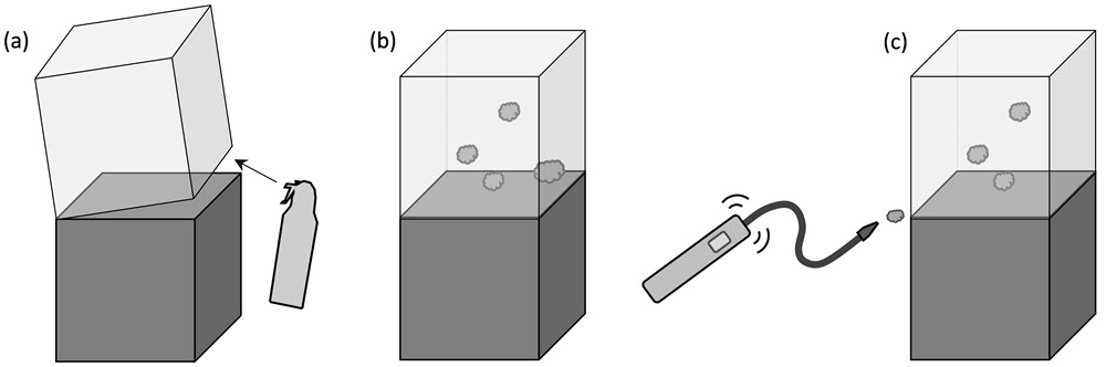
Protocol
This protocol for determining the airtightness of a display case or any other type of enclosure is based on the CO2 tracer gas method. Figure 13 illustrates the main steps in the procedure. To begin, it is best to run the test with an empty case to limit the number of influencing factors. If the aim is to have a very airtight case, it is suggested to look for leakage points and fix them before performing the experiment. Refer to the section Detecting points of leakage. There is also a checklist for the protocol in Appendix A.
© Government of Canada, Canadian Conservation Institute. 132731-0021
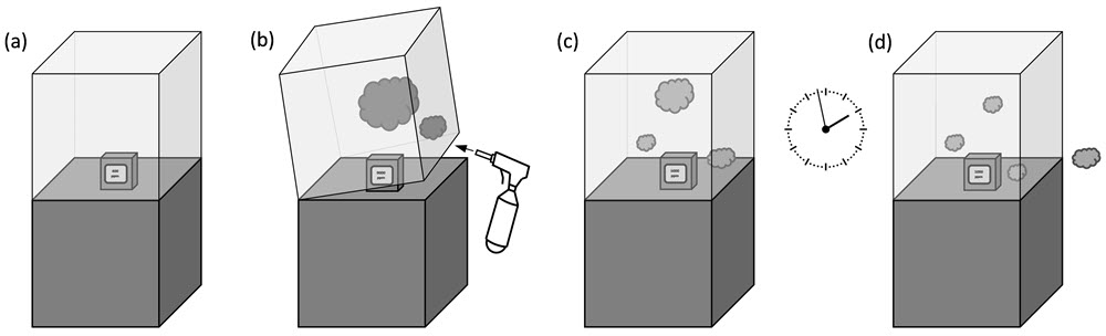
Figure 13. The basic steps for display case airtightness quantification with CO2: (a) install a CO2 monitor in the display case, (b) add CO2 tracer gas, (c) close the case as normally performed and (d) record the CO2 decay over time.
Record some aspects of the display case
Recording some details about the case design, environmental control, object composition and climate conditions (RH and temperature) can help to explain potential anomalies encountered in the CO2 decay trend.
- Take note if porous objects and/or plinths with significant internal volume (cavity) are present in the display case. An image of the tested case may become useful later for cross-checking details.
- Take note of the presence of silica gel and activated carbon in the environmental control compartment.
- Keep a record of the temperature inside the display case as the experiment progresses, using the CO2 monitor or another monitor if necessary.
- For storage cabinets or transportation boxes, take note if some objects are placed in smaller enclosures such as well-sealed plastic bags or cardboard boxes.
- Indicate the location of the case being tested (building and room).
CO2 monitoring data-logger set-up
- The data acquisition rate can be set to 30-minute intervals by default. This will provide sufficient resolution for leaky cases (AER higher than 1/day). The acquisition rate may be reduced to one to three hours for more airtight display cases (AER lower than 1/day).
- Calibrate the CO2 monitor according to the manufacturer’s instructions, if necessary. This can be performed a few hours or days before the experiment starts. The calibration is mandatory if more than one monitor is used.
- Place the monitor outside the display case and turn it on. Keep people away from the monitor to avoid an undesired source of CO2. This value will be used as the CO2 background level.
- Install the monitor in the display case. Air should circulate well around the monitor. If you have more than one device, you can also install one outside the case. Recording the CO2 level in different compartments can also help to understand the dynamics of the case, such as the time response of the moisture sorbent in the environment compartment (how effectively it may control the air volume of the display compartment of the case). When the display case has separate access to an environmental control compartment, it may provide an easier way to insert the CO2 monitor without having to open the display section.
Gas injection
- Close the display case, leaving as small an opening as practically possible for the injection of the CO2 gas. The small opening can be at the level of the environmental compartment.
- Inject CO2 to reach the predetermined concentration. The starting level should be in the range of 3000 to 6000 ppm. Starting at much below 3000 ppm may not give a sufficient decay range for the airtightness determination (especially for leaky cases), and there is no need to go above 6000 ppm.
- Seal or close the case in the usual manner when the desired internal CO2 level is reached. As much as possible, avoid activities around the display case that can affect the CO2 background level during the experiment.
As a rule of thumb, it is necessary to inject 2 g of CO2 for each 1000 ppm required per cubic metre. For example, if the aim is to generate a 4000-ppm concentration of CO2 in a 1 m3 case, you will need to inject 8 g of CO2. If you are using a 12 g cartridge, after an 8 g injection, the remaining 4 g will generate only 2000 ppm in another 1 m3 case.
Experimentation is required to determine how much time it takes to empty a CO2 cartridge with your injector device and then to estimate the time needed to reach a specific concentration. Keep in mind that some CO2 will also be released into the room during the injection. Adding an extension tube to the discharge nozzle can help to direct the gas into a small opening of the display case to minimize the spread of CO2 in the room.
You will notice when discharging CO2 that the injector head and the cylinder become very cold. This is normal and is explained by adiabatic expansion: a thermodynamic transformation due to a fast change in pressure. Some injectors do not have a protective outer sleeve, and the cylinder is held directly in your hand. For this type of equipment, take care not to expose skin to the cold metal cylinder. A neoprene sleeve is often provided with the injector kit for insulation.
Also note that when the environment is humid, frost may form on the discharge nozzle and block it. In this situation, it is necessary to wait until it warms up in order to resume.
A miniature, battery-operated fan is sometimes used to accelerate the dispersion of CO2. This can be especially useful for preliminary tests performed over a short period. It could be operated for the first 5 to 10 minutes, but not for the full duration of the test. A fan in a small enclosure can reduce the measured airtightness value, as demonstrated in Case study 4: the effect of a fan.
It is recommended to wait at least five minutes after adding the initial amount of CO2 to check if the concentration is sufficient. Inject additional CO2 if the level is too low, and reassess after an additional five minutes. Two options are available if the reading reaches the maximum scale of the monitor:
- accept that the test will take more time for the concentration to decay into the measurement range or
- attempt to disperse some gas by opening the case slightly until the desired concentration is achieved.
For the first option, it may take hours or even days to reach the measurement range of the monitor with excessive CO2 in an airtight case. The challenge with the second option is the delay between adjusting the concentration and reading the new value. It is easy to oscillate between having too much and too little CO2 until some experience is obtained with the test method.
Duration of the decay test
A simplified guideline for the duration of the test is as follows:
- Test for 7 to 16 hours (full working day or overnight) for preliminary results or a fabrication check.
- Test for four days for certification (including the stabilization period but excluding the period where the concentration is above the upper limit of the CO2 monitor).
Justification for the duration is detailed in Case study 5. Note that the stabilization period refers to the time required to reach a uniform initial CO2 concentration in the enclosure. This topic is discussed in the section Methods for calculating the airtightness as well as Case study 5: justification for the test duration.
End recording data
- If only one monitor is used, at the end of the test, place the CO2 monitor outside the display case to obtain useful data regarding the external concentration. As previously mentioned, keep people away from the monitor to avoid undesired sources of CO2. This extra value will be used to determine the average CO2 background level with beginning and end values.
- Download data from the CO2 logger to a spreadsheet program, such as Excel, for analysis.
Methods for calculating the airtightness
Two approaches are outlined for determining the enclosure airtightness: the two-point and the multi-point decay methods. The two-point decay method is useful for a quick assessment, such as a fabrication or assembly check. The multi-point decay method can be used for similar purposes as well as for certification. The multi-point decay method requires more data and typically more time; however, it yields results with higher accuracy. A review of these data points also helps to verify when the CO2 level is sufficiently uniform throughout the different parts of the enclosure. This is defined here as the stabilization period. In addition, the multi-point decay method highlights when a noisy (fluctuating) CO2 background starts to alter the smooth decay process. The two methods are described in greater detail below.
Airtightness calculation tool
CCI has created an airtightness calculation tool as an Excel workbook that illustrates the two approaches for determining enclosure airtightness. The tool uses example data with equations 5 and 6 to create graphs similar to Figures 14 and 15 in this Bulletin. Users can input their own data to produce customized graphs by downloading the file.
Two-point decay method
After collecting data that shows the tracer gas decay over time, the simple way to calculate the airtightness is using Equation 4 (Brimblecombe and Ramer 1983). This method involves taking data points (tracer gas concentrations and the measurement time) at the beginning and end of the period of interest. The starting point is chosen after stabilization of the tracer gas is reached in the enclosure, and the end point is when the concentration is at least 600 ppm higher than the background level in the room.
Equation 4:
Where:
N = airtightness (1/day)
ln = natural logarithm
Cin1 = internal concentration of tracer gas at the test onset (ppm)
Cin2 = internal concentration of tracer gas at the test end (ppm)
Cex = external (room) concentration of tracer gas (ppm)
Δt = duration between measurements of Cin (day)
The external CO2 concentration (Cex) can be defined by a measurement in the room immediately before or after the test or by using an average of both. If an extra data-logger is available, it is possible to determine an average CO2 background over the full duration of the test.
As an example, Figure 14 shows the CO2 decay in a 0.063 m3 plastic container that had no obvious visual gaps. One monitor was placed inside the container and another in the room. The acquisition rate was set to 30-minute intervals, and the average external concentration was 613 ppm. The injection started at approximately two hours, and a maximum level of 4222 ppm CO2 was reached at about three hours.
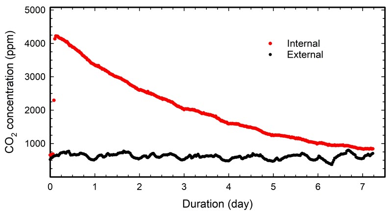
© Government of Canada, Canadian Conservation Institute. 132731-0022
Figure 14. CO2 decay in a plastic container, and the corresponding concentration in the room.
Table 1 presents five sets of two points taken from the data in Figure 14, and it shows the resulting variation in airtightness. Sets 1 and 2 represent a typical short-term evaluation of the airtightness during a single workday. Set 2 was selected as two points shifted by 30 minutes compared with Set 1. Set 3 also represents a short-term evaluation, but from an overnight period. Set 4 uses data spanning approximately four days (96 hours), knowing that this duration provides an accurate determination of airtightness. Set 5 uses an even longer time scale: from four hours into the test to the end time (127 hours). The end time corresponds to the time required to reach the end limit concentration (1215 ≈ 613 + 600 ppm). Consult Case study 5: justification for the test duration for the justification of the four days and the definition of end-limit concentration.
| Set | Cin1 (ppm) |
t1 (hour) |
Cin2 (ppm) |
t2 (hour) |
Duration (day) | N (1/day) |
|---|---|---|---|---|---|---|
| 1 | 4218 | 3.5 | 4015 | 9.5 | 0.25 | 0.23 |
| 2 | 4213 | 4 | 3976 | 10 | 0.25 | 0.27 |
| 3 | 4213 | 4 | 3512 | 20 | 0.67 | 0.32 |
| 4 | 4213 | 4 | 1591 | 96 | 3.83 | 0.34 |
| 5 | 4213 | 4 | 1215 | 127 | 5.13 | 0.35 |
Using Equation 4, the calculated airtightness varies based on the different pairs of points chosen from Figure 14 and listed in Table 1.
Example with set 1:
N = [ln(Cin1 − Cex) − ln(Cin2 − Cex)] / (t2 − t1)
N = (ln(4218 − 613) − ln(4015 − 613)) / ((9.5 − 3.5)/24)
N = 0.23/day
Set 1 indicates an airtightness of 0.23/day using data at 3.5 and 9.5 hours. Set 2 gives a slightly higher value of 0.27/day using readings at 4 and 10 hours. The delay of 30 minutes allowed an optimal mixing of gases within the enclosure. Set 3 covers a range of 16 hours (0.67 days) and gives an airtightness of 0.32/day. Set 4 provides an airtightness of 0.34/day with an end period of four days. Finally, set 5 gives an airtightness of 0.35/day using the longest time, spanning up to the practical limit of concentration. The difference in airtightness between sets 4 and 5 is only 3%, which confirms the accuracy obtained with a four-day period.
Multi-point concentration decay method
The second way to determine the airtightness is by considering all data using a graph in the form of ln(Cin − Cex) versus time. The slope of the regression line gives the airtightness. Note that the slope is negative since tracer gas is leaving the enclosure; however, the airtightness value is reported as positive. A spreadsheet program such as Microsoft Excel will assist in this regression analysis using a linear best fit. The data must be in the following format: the column for the x-axis is the time in days, and the column for the y-axis is the corresponding ln(Cin − Cex) value. The function “=Slope(Y1:Y2, X1:X2)” gives the overall airtightness.
An alternative to slope function is the linear “trendline” feature in the charting tools. This gives a linear equation where the slope and R2 are obtained. In this case, a high R2 (1 indicating a perfect straight line with no variation) represents stable monitoring and an absence of external influences on the decay process. An R2 below 0.990 is probably a sign of a non-linear relation. In this case, identify the possible cause, such as an unstable external environment or an unsuitable period selected for analysis. Redo the test if the possible cause is related to unstable CO2 decay at the beginning or the end.
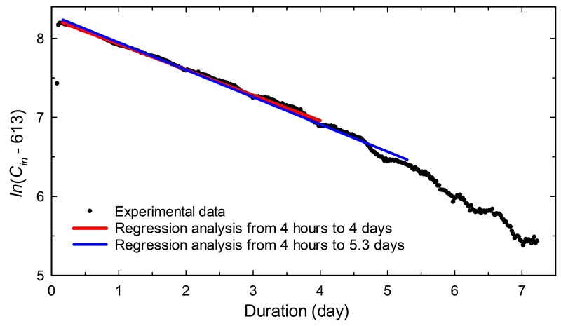
Figure 15 shows a plot of ln(Cin − 613) versus time using the same data as Figure 14. An airtightness of 0.32/day with R2 = 0.997 is obtained using the period of four hours to four days. With a period spanning from four hours to the end limit (5.3 days), an airtightness of 0.35/day is indicated with an R2 of 0.994. The difference in airtightness between these two regression analyses and the two-point methods (sets 4 and 5 in Table 1) is less than 5%. In Figure 15, after 5.3 days, experimental data does not follow a linear pattern due to the influence of the fluctuating CO2 background. This shows that the determination of the airtightness based on four days is accurate enough and an extra delay will not provide a better result.
The stabilization took about one hour, which is difficult to see in Figure 15. When it takes more time, such as many hours, the period becomes more obvious with the regression analysis. Consult Case study 6: multiple compartment display case for an example of a very long stabilization period with a two-compartment display case.
© Government of Canada, Canadian Conservation Institute. 132731-0024
Figure 15. CO2 decay in an enclosure expressed as the natural logarithm of CO2 concentration minus the external value in the room (613 ppm) as a function of time. Two regression analyses are shown (straight lines), spanning different periods, for the determination of airtightness.
Description of Figure 15:
The graph shows CO2 decay in an enclosure expressed as the natural logarithm of CO2 concentration minus the external value in the room (613 ppm) as a function of time. Experimental data show a rather linear decay with light fluctuations. Two regression analyses are shown, spanning different periods, from 4 hours to 4 days and from 4 hours to 5.3 days. Both regressions show a similar slope.
Reproducibility
As mentioned previously, the accuracy of the CO2 monitor gives an error in the range of 3% to 5% (consult Tracer gas monitoring and data-loggers), and it is reasonable to assume some drift of the sensor reading with time. Reproducibility is also affected by the opening of the enclosure between tests.
To examine the overall reproducibility of the airtightness determination, a dining hutch that was retrofitted to be more airtight was tested three times with three CO2 monitors. The results gave an airtightness reproducibility of 14%. Details of these tests are reported in Case study 7: error and reproducibility.
Calver et al. (2005) did a similar verification with an acrylic case by performing more than 25 tests and obtained a relative standard deviation (RSD) of 11%. English Heritage has tested approximately 400 display cases and defines a reasonable reproducibility of 20% for most cases, but some old hinged wooden cases can go up to 40% (Thickett et al. 2005; Thickett 2021).
Based on these three investigations, we can assume that from test to test, the conservative reproducibility of the airtightness values is in the range of 20%. For example, if the exact airtightness for a display case is 0.30/day, two measurements can give a result as low as 0.24 and as high as 0.36/day. Cases tested in the factory may show different airtightness values after being moved and installed in their final location. Also, keep in mind that the airtightness may decrease due to material fatigue or wear, deformation and misalignment.
Report the airtightness
The report should include the following information, when appropriate. Example data are provided using results presented in Figure 15.
- Include a description of the display case tested. Provide information such as location of the test, volume of the case and primary case materials, and give a description of the content if the case is not empty.
- Include the instrument used and indicate the protocol followed, such as this Technical Bulletin, International Organization for Standardization (ISO) standard 12569:2017 (ISO 2017) (specifying the sections used) or your own custom protocol.
- Include the figure of the natural logarithm of CO2 decay concentration minus the background as function of time. The time range used for the multi-point decay method should be visible in the figure. This will make it clear that the stabilization period, and data beyond the end limit, were excluded from the regression analysis.
- Report the external CO2 level from one reading or from an average of many readings (for example, CO2 background level is 613 ppm taken from two measurements: before injection and at the end).
- Report airtightness (for example, airtightness using CO2 is 0.32/day with R2 = 0.997 or Nco2 = 0.32/day, R2 = 0.997). Typically, only two significant figures are needed to report the airtightness (X.X/day, 0.XX/day or 0.0XX/day).
- Include the SD or the RSD if three or more tests were performed (consult Case study 7: error and reproducibility).
- Include the temperature and RH in the room or in the display case (recorded during the test, if pertinent). Significant temperature fluctuations may explain some deviations in the regression analysis (consult Case study 3: the effect of temperature on equilibrium CO2 content).
- Include the name(s) of who performed the test and the beginning and end test dates.
- Include a disclaimer, if pertinent, with the help of your lawyer. As an example: Display case #X was tested in your facility following protocol XYZ. Despite all precautions, we cannot guarantee the same airtightness when the case is in use. The reproducibility of the airtightness determination can be as high as 20%.
Airtightness as a specification
There is no worldwide standard for the airtightness of display cases despite the widespread use of standards for maintaining RH and pollutants within acceptable limits. Some museums, primarily in the UK, require an airtightness in the range of 0.1 to 1.0/day for new display cases and storage cabinets. Some have even requested 0.01/day. This section provides a brief review of specifications related to the airtightness.
In the UK, Padfield (1966) was the first to report a numeric value for the airtightness of a display case using water vapour. He found that conventional (well-made) cases have an airtightness of about 0.9/day. Later, Thomson (1977) performed airtightness measurements with water vapour and found an airtightness of 13/day for a loosely fitted glass display case and 1.3/day for a well-made case. Based on these findings, Thomson suggested that a well-made display case should have a leakage rate of no more than 1/day. He used this airtightness to develop his recommendation regarding the quantity of silica gel needed in display cases of a given volume.
The British Standards Institution (BSI) published recommendations for the storage and exhibition of archival documents (BSI 1977). This included specifications about the airtightness of display cases. In contrast to Thomson, this standard stated that a case design should allow sufficient air infiltration and that those points of ventilation should have dust filters. At that time, the focus was likely to minimize the risk of dampness (a common problem in the UK) and the risk of harmful compounds emanating from materials inside (Padfield 1966).
In 1989, the BSI updated its recommendations. The airtightness of display cases was related to RH control in the room:
- where RH is well controlled throughout the year, cases should have a vent with a dust filter; and
- where RH is not well controlled, cases should be airtight and include silica gel.
A major shift happened in the early 1990s when the Victoria and Albert Museum began requesting an airtightness of 0.1/day for their display cases (Cassar and Martin 1994). Their experiments were performed with nitrous oxide (N2O) as a tracer gas. The high level of airtightness was based on the fact that it became achievable by display case manufacturers without significantly affecting the cost of production or requiring extensive testing. Prior to the specification, they tested 13 display cases from different manufacturers. The average airtightness was 0.9/day with an SD of 1.1/day. The best two cases obtained an airtightness of 0.10/day and 0.15/day, and the two worst cases had 2.64/day and 3.36/day.
Careful attention to detail is obviously required to reach the 0.1/day target. To avoid unrealistic expectations, Cassar and Martin (1994) suggested, based on available funds, that objects needing tight RH control should be in airtight cases and that the others can be in less airtight cases.
An airtightness of 0.1/day also became a requirement from the Museums, Libraries and Archives Council in the UK (Holmberg and Kippes 2002). Later, it was found that it is not always easy to achieve this airtightness at a low cost (Thickett et al. 2005; Watts et al. 2007), since few display case makers have the required skills. This may explain why institutions around the world request an airtightness somewhere in the range of 0.1/day to 1.0/day. It is assumed that the airtightness is based either on a tracer gas of CO2 or N2O. In reality, most institutions do not currently specify airtightness for their display cases.
In 1999, the U.S. National Park Service (NPS) provided categories of display case seal effectiveness from unsealed to hermetically sealed. These were updated in 2020 and are shown in Table 2. The recommended airtightness of one AER per 72 hours (1/72 hours = 0.333/day ≈ 0.3/day) remained unchanged (AIC Wiki 2020).
| Degree of case seal | Air exchange rate approximations (per day as reference) based on NPS 1999 (original standard) | Air exchange rate (based on CO2 or N2O) from the AIC Wiki 2020 (replaces NPS 1999) |
|---|---|---|
| I. Unsealed | 1 AE per 1 hour or less (≥ 24/day) |
> 1.0/day |
| II. Moderately sealed | 1 AE per 24 to 36 hours |
≤ 1.0/day |
| III. Well-sealed | 1 AE per 72 hours or more |
≤ 0.3/day |
| IV. Very well-sealed | − | ≤ 0.1/day |
| V. Hermetically sealed | no air exchange | − |
It is important to specify the tracer gas, the equation and the method used for the airtightness determination in the request for proposals or in the report of the airtightness determination. Gas diffusivity conversion may be needed for very airtight cases (for example, if the focus of the airtightness is for water vapour control with silica gel and airtightness was determined with CO2). Consult Appendix B to know when this conversion is applied.
During the airtightness determination, some environmental parameters such as daily fluctuations of atmospheric pressure, light intensity and temperature can affect the result. The assembly of the display case may also change slightly during transportation or installation. This reproducibility issue is covered in Case study 7: error and reproducibility. Case makers may be forced to design for an AER lower than requested in order to fulfill the requirement with certainty. On the other hand, the client may accept some tolerance ranges. For example, an institution requests an airtightness of 0.30/day but, when tested in situ, an airtightness up to 0.50/day remains acceptable for the client. The targeted airtightness and tolerance range or rejection criteria should be clarified in advance by both parties.
It is important to keep in mind that the environmental stability of the room can have a significant impact on the airtightness determination. Improved performance may be observed for tests done in environments that are more stable than the final location of the enclosure. To avoid surprises, case fabricators should be aware of the environmental conditions at the client end. Fabricators should provide the temperature range or the logged temperature data during the CO2 decay measurement.
Since the optimization of environmental control in cases often relies on the specified airtightness, it is fair for institutions to indicate in their request for proposals proof of a specific airtightness obtained either at the factory or at its final location. The institutions may also verify the airtightness in situ themselves or ask for an independent evaluation of their case.
It may also be of interest to verify the stability of airtightness over time. Factors such as the aging of materials, frequency of accessing the inside, deformation and vibration can affect the airtightness. At the present time, no known warranty exists for the airtightness performance of cases after one or three years. A dialogue can develop between customers and case makers to verify the airtightness a few years after the installation and also to clarify who will be responsible for the retrofitting. This extra measurement and possible retrofit will come at an extra cost.
Overall, institutions should decide for themselves the level of airtightness that fulfills their needs. A common use of the airtightness value is for determining the amount of silica gel required for display cases and, in turn, the size requirements for silica compartments (consult Case study 1: specify an airtightness based on silica gel maintenance). For the other scenarios, the decision should be based on the potential risk of agents of deterioration in their context (consult Agents of deterioration). In some contexts, airtight display cases are not prescribed, and extra ventilation may even be needed (consult Case study 2: risk of lead corrosion in a display case made of oak).
Other considerations that may dictate the level of airtightness are mitigation options, design concept, tolerance range and budget. If the owner and the display case makers do not have the expertise to determine the airtightness of cases, a third party can be contacted. Alternatively, as a simplified option for specification, a criterion could be that the case should pass the paper test or that no leakage should be detected with leakage detection methods (consult Detecting points of leakage).
Case studies
Case study 1: specify an airtightness based on silica gel maintenance
In the UK, it is a challenge to maintain a dry environment for objects containing archaeological metals such as iron and copper alloys, particularly in a historic building. For this reason, silica gel is often used for passive humidity control in display cases (Figure 16).
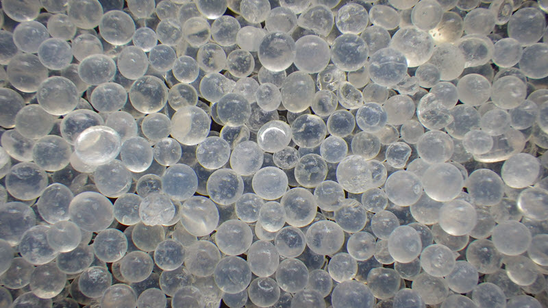
© Government of Canada, Canadian Conservation Institute. 132731-0026
Figure 16. Silica gel commonly used in display cases to control RH fluctuations.
Thickett and Luxford (2007) gave an example of an airtightness specification designed to support a specific environmental performance in this scenario. In a room, the RH was in the range of 60% to 90%. An old display case of 0.24 m3 was quite leaky and required 35 kg of silica gel to maintain a low RH inside. The performance target for new display cases was an RH level below 30% maintained for at least six months by using a reasonable amount of well-spread-out moisture sorbent. In this context, it was found that the new display cases should have an AER of 0.4/day or lower. Only 5.65 kg/m3 of silica gel was needed to fulfill the goal of this level of airtightness. As a bonus, they found that the RH stayed below 30% for almost a year.
Two hypotheses could explain this high performance, and both are related to parameters involved in Equation 1. The specific moisture reservoir (M) of the regular silica gel used was most likely equal to 2 g/kg for a 1% RH, since their methodology was based on Thomson (1977). More recently, Tétreault and Bégin (2018) found better performance of silica gel at RH below 30% (5.5 g/kg for a 1% RH). Knowing that the RH in the room was closer to 90% than 60% during the period of investigation (Thickett 2021), the second hypothesis is simply that the actual airtightness was closer to 0.2 than 0.4/day.
A similar approach was used by Stanley et al. (2003). They wanted to maintain RH inside a display case in the range of 40% to 60% while the room RH fluctuated from 35% to 84%, and they also wanted to limit the reconditioning of moisture sorbents to intervals between 6 and 12 months. Their target was a relatively easy to achieve airtightness of 1/day, using 20 kg/m3 of sorbent based on the recommendation of Thomson (1977).
Note that there is often a difference between theory and practice. One common reason is that many case materials and objects are hygroscopic, and they contribute to the humidity buffering effect. The RH fluctuations may appear better controlled when all components of the display are installed. On the other hand, if the temperature fluctuates too widely, the RH can fluctuate more than expected. This is due to the effect of the temperature on the moisture equilibrium of the different materials.
Another scenario is when a massive object is not equilibrated to its new environmentally controlled case. This could affect the overall RH in the case even if the silica gel was equilibrated to the desired target. A final difference in practice can occur with very airtight enclosures, where a correction factor is required to convert from the airtightness based on CO2 to that of water vapour. This is due to the difference of AER between diffusion and infiltration. Consult Appendix B.
Case study 2: risk of lead corrosion in a display case made of oak
Corrosion of lead is often reported when an object is in close proximity to oak, which can either be part of the display case material or part of another object. These two situations are shown in Figures 17 and 18. The main volatile compound emitted by oak is acetic acid, and lead is the most sensitive material to this acid. It is known that untarnished lead is less likely to corrode if the concentration of acetic acid is below 400 µg/m3. Tarnished lead will not corrode if the concentration of acetic acid is below 3000 µg/m3 (Tétreault et al. 1998), unless the patina or tarnish layer is not uniform or stable. In this case, corrosion may occur. The concentration of acetic acid emitted by uncoated red oak can reach 6700 µg/m3 in an airtight enclosure (Tétreault and Stamatopoulou 1997). The risk of lead corrosion is, therefore, obvious in the presence of oak. This highlights the issue of enclosure airtightness when the source of pollutants is inside.
© Government of Canada, Canadian Conservation Institute. 128118-0002
Figure 17. Brass-plated lead item corroded in a display case made of varnished oak. Note the deposits of white dust, which are assumed to be lead corrosion compounds.
© Government of Canada, Canadian Conservation Institute. 130062-0060
Figure 18. A bar of lead on exhibit mounted on a varnished wood base and inside a display case. The lead bar is corroding, most likely due to the acidic volatiles emitted by the wood and varnish.
The risk of lead corrosion in the presence of oak can be assessed with the help of Equation 3. We can establish the concentration of acetic acid in the case as a function of the airtightness and at different loads (the ratio of the emissive surface to the volume of the case), as shown in Figure 19. A mass transfer coefficient of 0.18 m/h for the acetic acid–oak system is chosen based on the work of Ryhl-Svendsen and Glastrup (2002) and Smedemark et al. (2020).
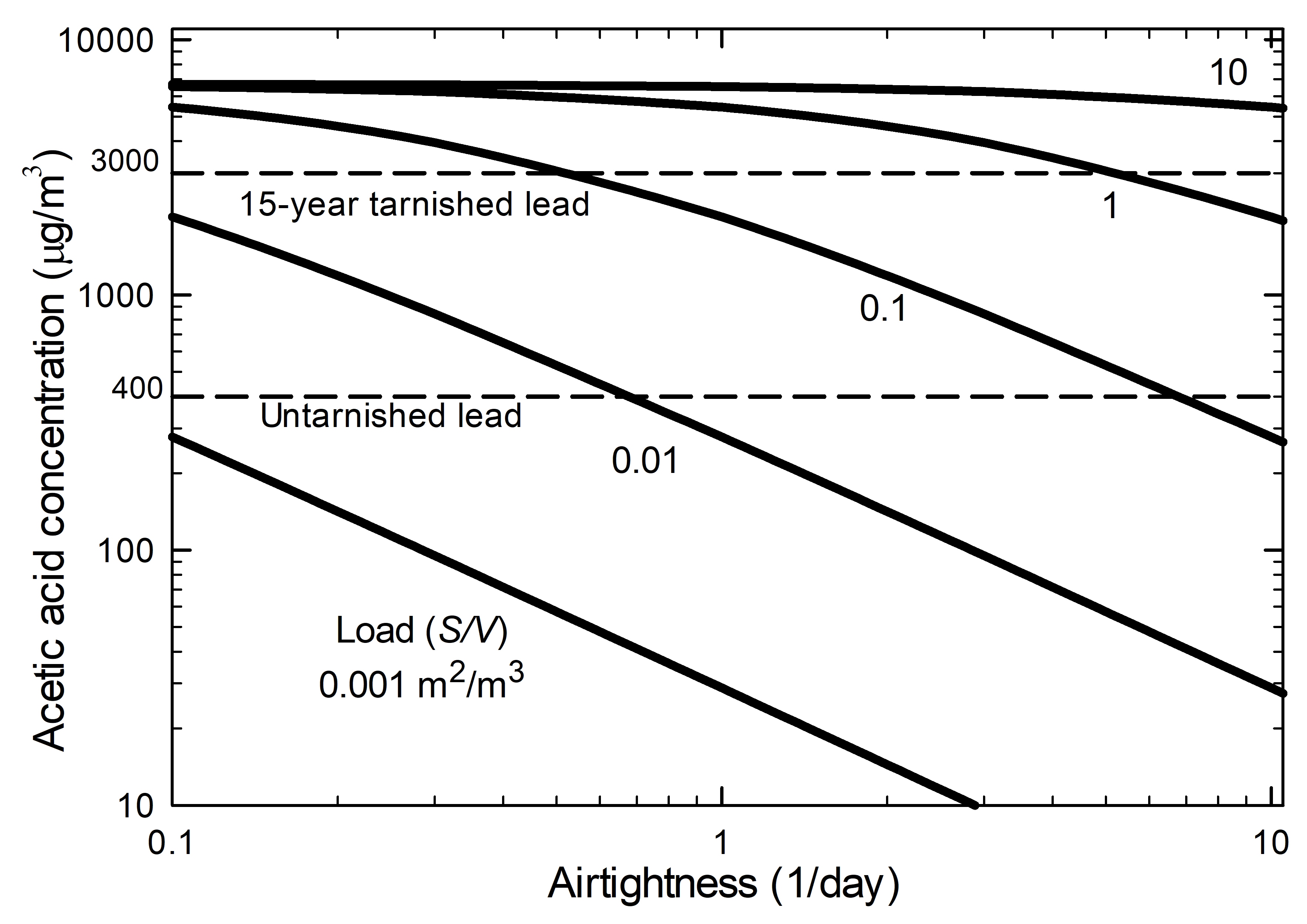
© Government of Canada, Canadian Conservation Institute. 132731-0027
Figure 19. Concentration of acetic acid emitted from oak in an enclosure as a function of the airtightness and based on different loads.
Description of Figure 19
The graph shows the relationship between the acetic acid concentration in µg/m3 (y-axis) and the airtightness of an enclosure containing oak panels at different loads (x-axis is an airtightness of 1/day). For a specific load, an increase of the airtightness value gives a smaller acid concentration. Further reductions of the concentration occur with smaller loads. Two reference concentrations are indicated on the figure: one at 400 µg/m3 and the second at 3000 µg/m3. These two concentrations represent the concentration limit to prevent corrosion for untarnished and tarnished lead, respectively. Untarnished lead is at risk of corrosion within an enclosure having a load of oak of 0.01 m2/m3 if the airtightness value is below 0.7/day. In those conditions, tarnished lead is not at risk. However, tarnished lead becomes at risk if the load is 0.1 m2/m3 or higher.
If we assume a volume of 1 m3, each load in the figure represents the surface of an oak panel:
- 10 m2/m3 = 10 panels of 1 m2
- 1 m2/m3 = a panel of 1 m2
- 0.1 m2/m3 = a panel of 32 cm × 32 cm
- 0.01 m2/m3 = a panel of 10 cm × 10 cm
- 0.001 m2/m3 = a panel of 3.2 cm × 3.2 cm
Two reference concentrations are indicated on the figure: one at 400 and the second at 3000 µg/m3. These two concentrations represent the concentration limit to prevent corrosion for untarnished and tarnished lead, respectively.
From Figure 19, we can see that a small 3.2 cm × 3.2 cm uncoated oak piece is unlikely to cause corrosion at any enclosure airtightness. A 10 cm × 10 cm oak piece can already be a potential problem for untarnished lead with an enclosure having an airtightness below 0.7/day. Stable tarnished lead becomes at risk of corrosion with a piece of 32 cm × 32 cm at an airtightness below 0.5/day. Still, coated oak remains a potential risk for lead in many circumstances.
Often, wood used for a display case is coated. Dry emulsion coatings can reduce the acetic acid emission rate of oak easily by 90% or even more (Tétreault and Stamatopoulou 1997). If we assume a reduction of 90% in our scenario, consequently, the mass transfer coefficient of the coated oak panel becomes 0.018 m/h (10 times smaller than uncoated oak). Figure 19 can still be used for coated oak, but the load needs to be considered as 10 times lower. For example, an acetic acid level is 2021 ppb with an oak load = 0.1 m2/m3 and N = 1/day. For coated oak with an adjusted load (0.01 m2/m3), the level of acetic acid reaches only 277 ppb. Note that some oil-based paints can release much more acid than the oak itself.
The use of Equation 3 has some limitations. The mass transfer coefficient may shift as the conditions of use (airtightness, emission rate, surface and volume) differ from its experimental condition. The equation also assumes no sorption of any product inside the case and no outside pollutant.
It is evident in Figure 18 that the bar of zinc in the background is similarly mounted and exposed to the same volatiles within the display case but is not showing obvious signs of corrosion. Zinc is much more resistant to the corrosive action of acetic acid (Tétreault 2003, p. 26).
Case study 3: the effect of temperature on equilibrium CO2 content
Temperature fluctuations can affect the airtightness value by causing pressure differences between the enclosure and the room, and they can have a further influence by changing the equilibrium CO2 content of various materials. The equilibrium concentration between CO2 in the air and a solid material is similar to the concept of equilibrium moisture content (EMC), which is well known by conservators. For a specific temperature and air CO2 concentration, materials may have different CO2 content. As the CO2 concentration decreases, the absorbed CO2 slowly desorbs. This absorption-desorption process could affect the airtightness measurement. One material having a high affinity to absorb CO2 is concrete. It absorbs 10 times more than wood and books (Kigawa et al. 2003). Activated carbon is also a good CO2 absorber, while silica gel has half its capacity (Berlier and Frère 1997).
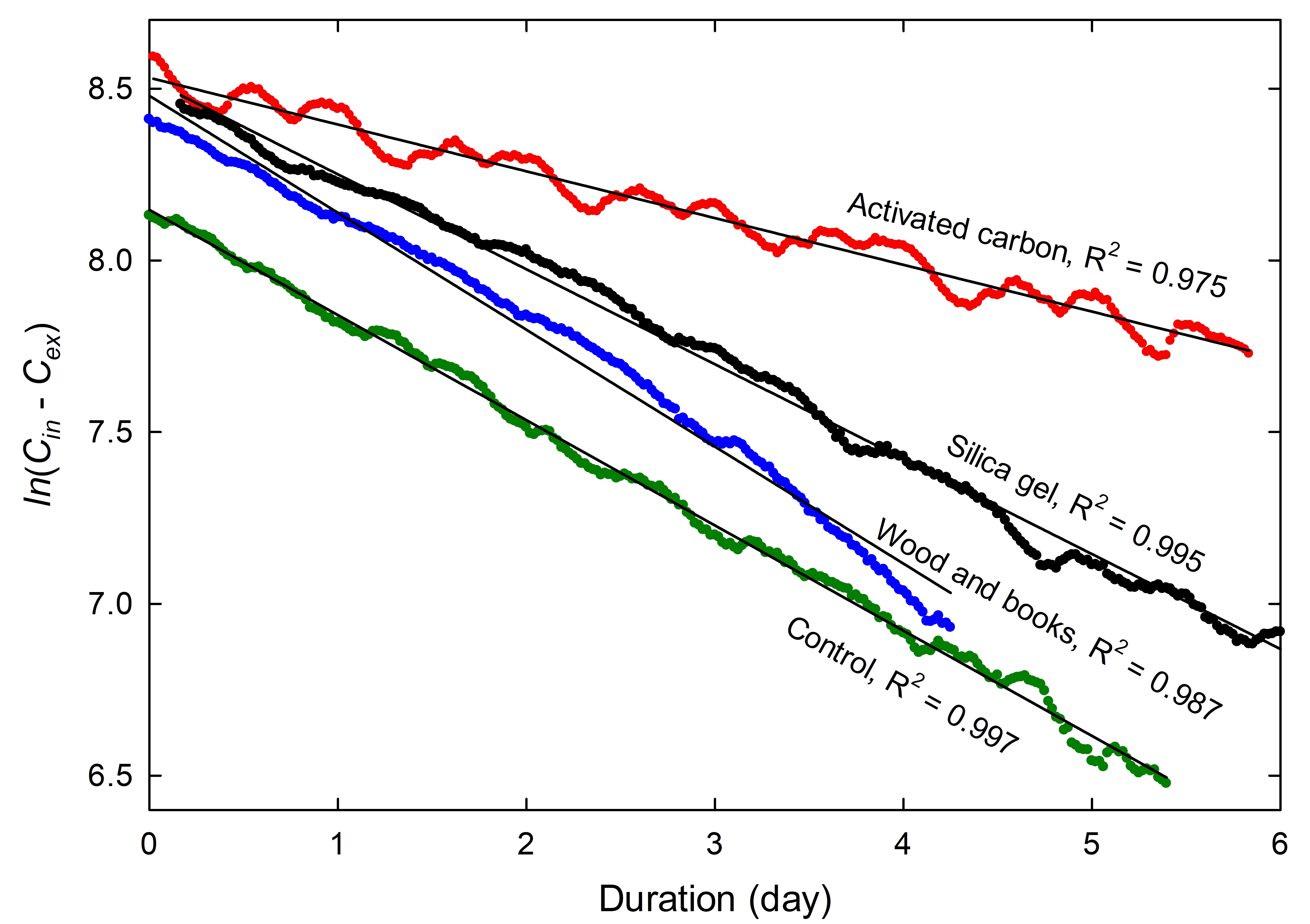
© Government of Canada, Canadian Conservation Institute. 132731-0029
Figure 20. Natural logarithm of CO2 decay in a plastic container having different materials under a temperature fluctuation range from 17.0°C to 21.0°C. Some slopes have been shifted to better distinguish the fluctuation caused by each material.
Figure 20 shows the natural logarithm CO2 decay in a 0.063 m3 plastic container with different contents. Three materials were used in separate experiments: 0.380 kg of activated carbon (made from coconut shells), 0.66 kg of silica gel (one cassette of PROSorb) and a mixture of 1.49 kg of pine boards and 1.87 kg of books. The control was simply an empty container. During the tests, daily temperature fluctuations were maintained in the range of 17.0°C to 21.0°C. From the measurements, it is evident that the slopes for the enclosure containing silica gel and the one containing wood and books are similar to the control. Thickett (2012, pp. 106–107) also found no difference in the airtightness value with silica gel. The result with activated carbon is different in two ways, as it has the weakest slope (best implied airtightness) and the least stable decay (lowest R2).
The behaviour of the case with activated carbon is interesting from a theoretical perspective. Activated carbon has a high surface area, which increases sorption capacity and enables a high rate of gas adsorption and desorption. With its greater surface area, the gas reaches a new equilibrium faster when the temperature or gas concentration in the air changes. In a CO2 decay test, the gas spreads throughout the enclosure after injection, and some CO2 is adsorbed by materials due to their respective affinity. As the CO2 decays over time by leakage from the enclosure, the adsorbed gas in materials is slowly released. This consequently slows the decay and incorrectly implies better airtightness.
As mentioned previously, the experiment with activated carbon shows the highest daily fluctuation. This variability in the slope is well synchronized with the temperature fluctuation, as shown in Figure 21 (left). In the same figure (right), the case containing wood and books shows minimal impact on the daily temperature changes. There is also a smooth long-term deviation of the slope, which is more obvious in Figure 20.
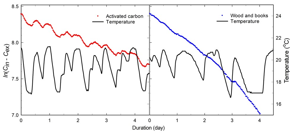
© Government of Canada, Canadian Conservation Institute. 132731-0031
Figure 21. Natural logarithm of CO2 decay in a plastic container having activated carbon (left) and wood and books (right) under a temperature fluctuation range from 17.0°C to 21.0°C.
Description of Figure 21
This figure contains two graphs showing the natural logarithm of CO2 decay in a plastic container with activated carbon (on the left) and with wood and books (on the right). Small temperature fluctuations are present during the measurement period. For the container with activated charcoal, the CO2 decay is moderate over time; however, significant fluctuations are synchronized with the temperature changes. The container with wood and books shows almost no fluctuations, but the decay is faster.
A repeat of the CO2 decay test with the same materials under a stable temperature (17.0°C to 18.0°C) improved R2 for all slopes, as shown in Table 3. The implied airtightness of the case containing activated carbon was still better than the control; however, not to the same extent as with greater temperature fluctuations (shown graphically in Figure 22). The AER under high and low temperature fluctuations are respectively 59% and 38% lower than the control. This incorrect determination of the airtightness due to activated carbon is independent of the stabilization period. For this reason, it is recommended to measure the CO2 decay with an empty enclosure or at least without activated carbon.
| Material in the container | Airtightness (1/day) of the container subject to large temperature fluctuations from 17.0°C to 21.0°C | Airtightness (1/day) of the container subject to small temperature fluctuations from 17.0°C to 18.0°C |
|---|---|---|
| Activated carbon | 0.14, R2 = 0.9720 | 0.21, R2 = 0.997 |
| Silica gel | 0.28, R2 = 0.9948 | 0.28, R2 = 0.997 |
| Wood and books | 0.34, R2 = 0.9870 | 0.30, R2 = 0.999 |
| Nothing (control) | 0.31, R2 = 0.9974 | 0.33, R2 = 0.999 |
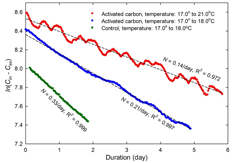
© Government of Canada, Canadian Conservation Institute. 132731-0033
Figure 22. Natural logarithm of CO2 decay in a plastic container with activated carbon under high and low temperature fluctuations compared to the control.
Case study 4: the effect of a fan
The use of a fan inside an enclosure may seem like a good solution for accelerating the mixing of air and reducing the stabilization period; however, it is important to consider the other effects of air circulation. To verify the potential impact of the fan on airtightness measurements, two tests were performed with a direct current fan (12 volt, 0.24 ampere) installed in a 0.063 m3 plastic container. One test involved the fan running at 1.5 volt (low speed) and the second at 4.5 volt (medium speed). A 12 cm diameter tall glass cylinder was placed in the centre of the container in hopes of creating a circular flow. The fan was turned on for a limited time, well after the stabilization period was completed.
Figure 23 shows two natural logarithm decays with increasing slope when the fan was activated, especially at medium speed. This clearly shows the effect of the fan on airtightness for a display case of small volume. In practice, a low-speed fan may not significantly interfere with the airtightness measurement of large cases. As a precaution, the use of a fan should be limited to the first 5–10 minutes as a means of reducing the stabilization period.
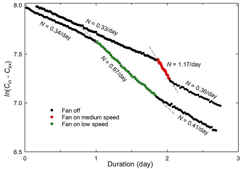
© Government of Canada, Canadian Conservation Institute. 132731-0035
Figure 23. Effect on the airtightness of a 0.063 m3 plastic container when a fan is turned on medium versus low speed. The experiment was performed with the fan speeds activated in the middle of the decay process.
Description of Figure 23
This figure shows two natural logarithm plots indicating linear CO2 decay over time. Approximately halfway through the measurement period, a fan is activated to circulate air. The decay increases slightly with the fan running at low speed; the decay increases much faster when the fan is running at medium speed. When the fan is turned off, both decay curves return to their initial rate.
Case study 5: justification for the test duration
In the section Duration of the decay test, two duration periods were proposed: less than a day, such as 7 to 16 hours for preliminary results or a fabrication check, and four days for the certification. The complete decay of CO2 in an enclosure may take much longer. For a very airtight case, it may take more than 10 days to reach the average CO2 concentration in the room. Fortunately, the CO2 concentration does not have to reach the background level (room) for a valid test. The test duration can be much shorter with a sufficient amount of accurately recorded data. This depends on the following factors:
- CO2 initial level and end level,
- stabilization period of the CO2 level in the display case,
- critical change in the decay,
- the minimal data acquisition number and
- expected airtightness.
As mentioned previously, the initial CO2 level should be in the range of 3000 to 6000 ppm. There is also a practical limit at the end of the test. The CO2 concentration should not be lower than approximately 600 ppm above the average background level. For example, if a level of 550 ppm is measured in the room, the end limit is 1150 ppm (550 + 600). If less than 600 ppm is added to the background, CO2 levels in the display case are more easily affected by fluctuating CO2 in the room. For this reason, data recorded below this end limit is usually not considered for the determination of the airtightness. It is best to start with a CO2 concentration near 6000 ppm when the background level in the room is much higher than 1000 ppm. This will ensure a proper test duration period.
The stabilization or the homogenization of the gas depends on the size and the design of the display case. Some objects or enclosure materials may absorb the CO2 and release it later. Display cases may contain two or more compartments, such as an environmental section, an empty display mount or objects wrapped in airtight plastic bags, which can take time to reach a uniform CO2 level. This stabilization can take from a few minutes to many hours. Thickett (2012, p. 103) reported that it can take up to 14 hours depending on the complexity of the case design. Case study 6: multiple compartment display case shows an example where stabilization of a two-compartment case occurs after 38 hours. Data recorded during the stabilization period is not included in the airtightness determination. The CO2 concentration reached after the stabilization period becomes the CO2 starting level.
One condition that is important to fulfill for the airtightness determination is to reach a significant CO2 decay after a predetermined period. This could be a challenge for very airtight enclosures. A significant decay can be defined as a 20% loss of the CO2 start level. This decay of 20% is based on the issue of the reproducibility of the technique (consult Case study 7: error and reproducibility). For example, if the CO2 start level is 5000 ppm (after stabilization), a 20% loss is 4000 [5000 × (1.00 − 0.20)]. If the significant decay of 20% is not reached during the experiment, the airtightness could be considered acceptable even if it cannot be measured accurately.
In addition to reaching a minimum decay of 20% from the starting concentration, a minimum of 20 evenly distributed data points is recommended in order to generate a useful trend. The quality (linearity) of the trend line is assessed on a semi-natural logarithm plot by a coefficient of multiple determination (R2) higher than 0.990. After the stabilization period, 10 hours of data recording is needed if the sampling rate of the monitoring data logger is 30 minutes (20 hours of data with a sampling rate of 1 hour). These 20 data measurements also give a high confidence with respect to the quality of the result for certification.
Many people will expect to see an extended decay, not just a 20% loss of CO2. If time permits, another milestone is to let the test run until reaching the half-life decay (half-decay). This is a concept frequency used for an exponential decay process. If the CO2 start level is 5000 ppm and the background level is 500 ppm, the half-decay is 2250 ppm [(5000 − 500)/2]. Of course, the final milestone, if more time is available, is when the decay reaches the CO2 end limit level (500 + 600 ppm) described earlier.
If the display case to be tested is expected to meet some requirements, such as an airtightness below 0.3 per day, the duration can be planned accordingly. Equation 5 helps to set up the experimental conditions and to predict the duration.
Equation 5:
Where
t = duration of the test for a specific target concentration (day)
Cin1 = start concentration after stabilization (ppm)
Cex = concentration of the background (ppm)
Cin2 = targeted concentration (ppm) such as 20% decay, half-decay or end level (Cex + 600 ppm).
N = airtightness (1/day)
The equation assumes the time at Cin1 is 0 days.
Three scenarios are proposed below based on a CO2 start level of 5000 ppm, CO2 background level of 500 ppm and the desired airtightness set at 0.30/day.
• Time to reach 20% decay:
t = {ln(5000 − 500) – ln[5000 × (1− 0.20) – 500]} /0.30 = 0.84 days
• Time to reach half-decay:
t = (ln(5000 − 500) – ln{[(5000 − 500) / 2] – 500}) /0.30 = 3.1 days
• Time to reach end limit:
(Cex + 600 ppm): t = {ln(5000 − 500) – ln[(500 + 600) – 500]} /0.30 = 6.7 days
Four days should allow enough time for adjusting the initial CO2 level, for stabilization and for reaching the half-decay. This is the reason why the certification is based on a four-day duration. This four-day period excludes any time where the CO2 level is beyond the detection range. There is sufficient data in four days of measurements to select a segment offering a high R2 (for example, if some unexpected shift happens due to changing environmental conditions, a CO2 background level change or failure of the seals).
Figure 24 shows the decay milestones for a starting CO2 level between 3000 and 6000 ppm based on Equation 5. An end limit was set at 1100 ppm to avoid the influence of the fluctuating background level set at 500 ± 300 ppm.
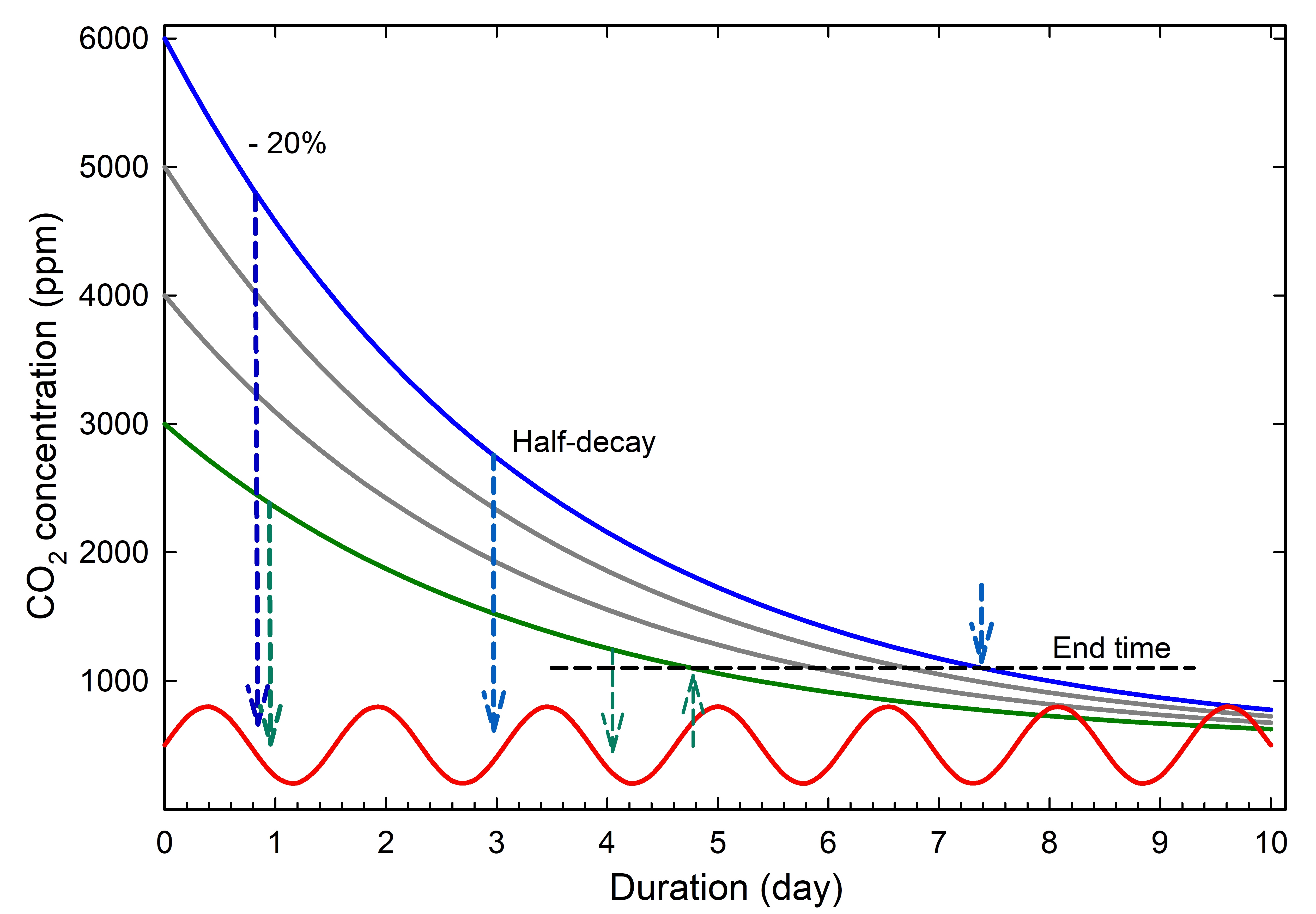
© Government of Canada, Canadian Conservation Institute. 132731-0037
Figure 24. Decay of CO2 concentration in an enclosure having an airtightness of 0.30/day, starting at different levels. The figure shows how much time it takes to reach a 20% loss, half-decay and the practical end limit. The daily CO2 external fluctuation is shown in red.
Description for Figure 24
The graph shows the decay of CO2 concentration in parts per million (y-axis) in an enclosure over time, starting at different concentrations. The x-axis is the duration in days. The lines indicate how much time it takes to reach a 20% loss, half-decay and the practical end limit for each example. If the initial CO2 level in the enclosure is 6000 ppm, it takes approximately 0.8 days to reach a reduction of 20%, 3 days to reach half-decay and 7.3 days to reach the end limit. If the initial CO2 level in the enclosure is 3000 ppm, it takes about 1 day to reach a reduction of 20%, 4 days to reach half-decay and 4.8 days to reach the end limit.
Case study 6: multiple compartment display case
It is common to have enclosures with multiple interconnected compartments. This can be a two-compartment display case where the object is placed in the top section and environmental control materials are placed in the bottom section, hidden from view. Inner enclosures can also be present in display cases and play the role of a box in a box. These inner spaces could consist of a fragile object encapsulated in its special case, an empty mount used to elevate a small object or even the object itself with an internal void, as shown in Figure 25. The concept of a box in a box provides added stability to the inner enclosure environment, especially with respect to RH fluctuations. The disadvantage is that multiple enclosures can cause a long stabilization period since CO2 equilibrium must be reached in all subspaces.
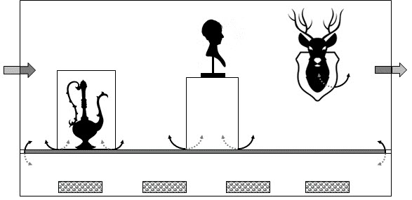
© Government of Canada, Canadian Conservation Institute. 132731-0039
Figure 25. A display case example showing internal volumes, from left to right: an object encapsulated, a mount to elevate a small object and an object having a void inside. A compartment in the bottom of the case is used for environmental control, where moisture and pollutant sorbents can be inserted. Small arrows show the slow air movement between the main enclosure and the smaller internal enclosures.
An empty two-compartment display case was investigated to demonstrate the effect of multiple compartments on the stabilization period. The case was made of Plexiglas and wood (Figure 26), with a total volume of 0.53 m3. The top chamber had a volume of 0.27 m3 and the base, 0.25 m3. The interface between the two compartments was expected to allow sufficient air movement. A CO2 level of 480 ppm was measured as the background level in the room, and two CO2 monitoring data-loggers were installed in the top and bottom parts of the case, respectively. The CO2 tracer gas was injected in the bottom section.
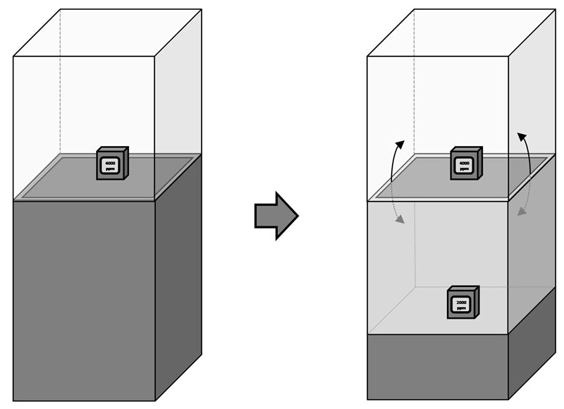
© Government of Canada, Canadian Conservation Institute. 132731-0040
Figure 26. Two-compartment display case. As shown in the right case, the top is the display area, and the bottom part can contain silica gel to control the RH in the overall case. Two small arrows show the slow air movement between the two parts.
Figure 27 shows the evolution of the CO2 in the two compartments of the display case as a direct reading of the CO2 and as a natural logarithmic value. The two graphs show, initially, a high level of CO2 at the bottom part of the case, where the CO2 was injected, and a low level in the top section. With time, they converge to a common value, and they reach the same decay rate after 38 hours. Airtightness of the overall case was 0.06/day with R2 = 0.995, using the multi-point decay method for the period of 38 hours to 4 days.
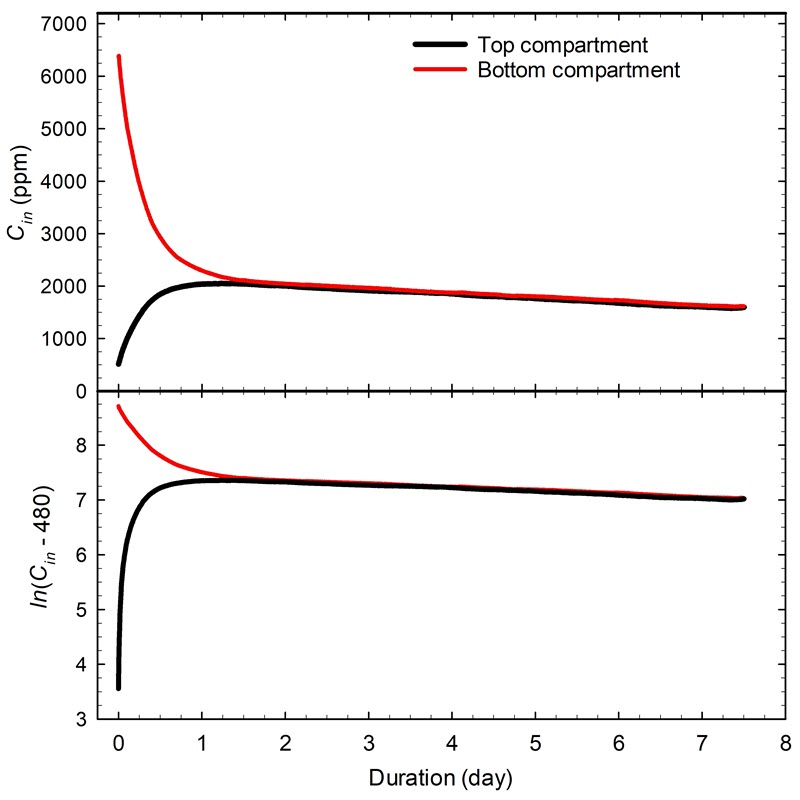
© Government of Canada, Canadian Conservation Institute. 132731-0041
Figure 27. Evolution of CO2 levels in two compartments of the display case shown as a direct reading of the CO2 level in ppm (top) and as natural logarithmic value (bottom).
With this display case design, a fundamental error is easily made in the airtightness determination if the two-point decay method is used without evaluating an extended decay. An airtightness of 1.06/day is found by using the two points at two hours (erroneous expectation of stabilization) and at one day for a short-term evaluation. The two-point decay method gives an airtightness of 0.32/day if four days is used instead of one day. Obviously, if the stabilization period is not considered, this can cause a substantial error in the airtightness value. It is also unlikely that a fan will be able to stabilize the CO2 concentration in both compartments.
The AER between the top and bottom parts of the display case can be determined with the use of two CO2 monitors. Assuming that the AER between the interior and exterior is much smaller than the AER between the top and bottom parts, the AER of the latter is found by replacing ln(Cin − Cex) by ln(Cin bottom – Cin top). The AER between compartments is 2.90/day with R2 = 0.999 for the linear range of 0.3 to 1.3 days, as shown in Figure 28.
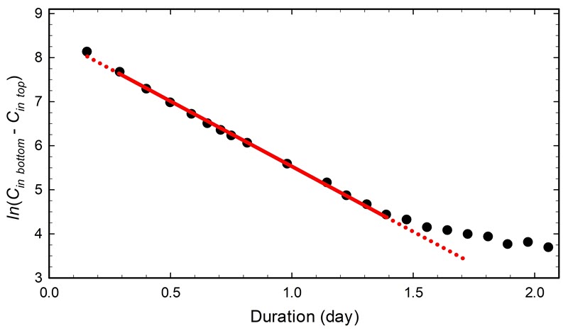
© Government of Canada, Canadian Conservation Institute. 132731-0043
Figure 28. Natural logarithm of the CO2 concentration difference between the two parts of the display case.
Since this display case is well protected against external agents with an airtightness of 0.06/day, the air movement of 2.90/day between the environmental control compartment and the display area is sufficient. However, it is not possible to determine from these results whether the main leak is from the top or the bottom part of the case.
Case study 7: error and reproducibility
Any analytical technique contains uncertainties due to user errors, accuracy and stability of the instrument as well as variability of the measured subject. This case explores those issues with a dining hutch cabinet as the enclosure. A 0.2 m3 dining hutch was newly retrofitted to be more airtight for the airtightness determination. As a first step, only one CO2 monitor was placed in the middle (Figure 29). The multi-point decay method gave an airtightness of 0.44/day with R2 = 0.991. The airtightness value can vary significantly with the two-point decay method, depending on which data points are selected, even in the linear range. Considering the extreme scenarios, the airtightness may be 16% better (inverted triangle points) or 13% poorer (triangle points), as shown in Figure 30.
© Government of Canada, Canadian Conservation Institute. 132731-0045
Figure 29. Schematic of an antique wooden dining hutch containing three evenly dispersed CO2 monitors. Only the upper section was monitored, since the lower drawers or cupboards were not connected to it.
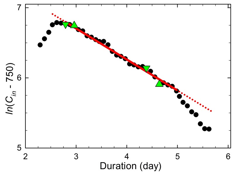
© Government of Canada, Canadian Conservation Institute. 132731-0046
Figure 30. CO2 decay in the dining hutch. The red line is the trend for the multi-point decay method. For the two-point method, the pairs of triangle points denote the extreme values: upright triangles for the higher slope and inverted triangles for the lower slope. The CO2 background level is 750 ppm.
As a further investigation with the same dining hutch, three CO2 monitors were introduced, and the cabinet was tested three times. Each time the hutch was opened for the injection and resealed. The three monitors were placed in different locations, as shown in Figure 29. The results with the multi-point method are shown in Table 4. The first test with the three monitors gives an airtightness of 0.44/day with an SD of 0.03/day or an RSD of 7.4%. The second and third tests give an airtightness of 0.52/day and 0.38/day with an RSD of 5.2% and 3.9%, respectively. The average airtightness by considering the three tests is 0.44/day with an RSD of 14%.
| Monitor | Test 1 | Test 2 | Test 3 |
|---|---|---|---|
| M1 | 0.426 | 0.517 | 0.360 |
| M2 | 0.415 | 0.488 | 0.386 |
| M3 | 0.476 | 0.541 | 0.385 |
| Average | 0.44 | 0.52 | 0.38 |
| Standard deviation | 0.03 | 0.03 | 0.02 |
| Relative standard deviation (%) | 7.4 | 5.2 | 3.9 |
Acknowledgements
The authors wish to thank Jennifer Herrmann from the U.S. National Archives and Record Administration, Eric Breitung and Alayna Bone from The Metropolitan Museum of Art and David Thickett from English Heritage for their comments during the revision process. The authors are also thankful for the replies from various people during a consultation on the Global Conservation Forum.
Appendix A: Airtightness checklist
Check for overall, fixable leaks requiring no specialized instrumentation.
- Verify that there are no major visible points of leakage by checking:
- interfaces between mated surfaces, such as glazing panels, doors and structural elements;
- around access points, such as the sorbent compartment door;
- gaskets and sealants that are poorly fitted, degraded or missing;
- keyholes;
- through-holes for electrical wires, lighting components or other accessories; and
- loose, distorted or missing fasteners.
- Verify that there are no points of leakage large enough to permit the passage of a credit card or sheet of printer paper.
Check for airtightness with the CO2 method.
- Record all pertinent display case information.
- Note if porous objects and/or plinths with a significant internal volume (cavity) are present in the display case. An image of the tested case may become useful later for cross-checking details.
- Note the presence of silica gel and activated charcoal in the environmental control compartment.
- Keep a record of the temperature and RH inside the case.
- For storage cabinets or transportation boxes, note if some objects are placed in smaller enclosures such as a well-sealed plastic bag and cardboard boxes.
- Indicate the location of the case being tested (building and room).
- Record background CO2 while minimizing disruption during the measurement.
- Place one or more calibrated monitors inside the display case, allowing for proper air circulation and a proper data acquisition rate for the length of the experiment.
- Close the display case.
- Inject CO2 into the case using as small an opening as possible to create a starting concentration in the range of 3000 to 6000 ppm.
- Seal the display case.
- Remember that the stabilization period can take up to 40 hours, depending on the design of the case.
- Allow sufficient time for a critical change in decay.
- When the experiment is finished, record a final background reading.
Appendix B: Graham’s law of diffusion
Leakage is often driven by airflow processes. This significant air movement is due to a difference in outside and inside air pressure, primarily caused by atmospheric pressure and temperature variations. When there are fewer or smaller gaps and holes and when the environment is more stable, the diffusion modes may become more significant in the overall leakage. The diffusivity of large acrylic glazing or (engineered) wood panels in a display case may become the leading contributor of the AER if no major gaps and holes are present.
It may be necessary to consider a correction to the airtightness value when the diffusion mode dominates the overall leakage process. This correction is based on Graham’s law of diffusion. Often, the airtightness is determined with a tracer gas that is different from the gas of interest. For example, when the airtightness of an enclosure is obtained with CO2 tracer gas, it is necessary to apply the result to the control of water vapour using the optimal amount of silica gel. The two gases have different rates of diffusion that define their own respective airtightness values. Graham’s law of diffusion (Equation 6) can transpose the airtightness value from the tracer gas to the gas of interest.
Equation 6:
Where
AER = air exchange rate (1/day)
MW = molecular weight (g/mol)
1 and 2 = gases 1 and 2
For example, if an airtightness of 0.100/day is obtained with CO2 as the tracer gas, the value becomes 0.156/day [0.156 = 0.100 × square root of (44/18)] for the AER of water vapour. Consult Table 5 for a list of AER conversions. When considering only the diffusion mode, if a max AER for water of 0.1/day is targeted and the tracer gas used for the airtightness determination is CO2, then the measured AER needs to be below 0.064/day (0.100 ÷ 1.563 = 0.064).
| Gas of interest | Molecular weight (g/mol) | Conversion factor |
|---|---|---|
| Carbon dioxide | 44.01 | 1.000 |
| Water vapour | 18.02 | 1.563 |
| Oxygen | 32.00 | 1.173 |
| Acetic acid | 60.05 | 0.856 |
| Formic acid | 46.03 | 0.978 |
| Hydrogen sulfide | 34.08 | 1.136 |
| Ozone | 48.00 | 0.957 |
| Nitrogen dioxide | 46.00 | 0.978 |
| Nitrous oxide | 44.01 | 1.000 |
| Sulfur dioxide | 64.01 | 0.829 |
In practice, no correction is required when the AER is above 1/day; possibly, a partial correction could be pertinent below 0.3/day if the internal pressure is stable in the enclosure. Daily fluctuations of atmospheric pressure, light levels and the temperature may cause a difference in pressure between the room and the enclosure. Infiltration and exfiltration become the dominant mechanisms when these fluctuations are important.
In a stable environment, a conservative approach suggests considering a contribution of the diffusion of 50% in the overall leakage for airtightness measured below 0.3/day. For example, if the AER measured with CO2 is 0.100/day and the focus is on the control of RH in the case, the overall AERwater becomes 0.128/day [(0.5 × 0.1) + (0.5 × 0.156)].
If we consider a possible experimental error up to 20% (consult Case study 7: error and reproducibility), it may be safer to consider an AERwater of 0.154/day (0.128 × 1.2) in the determination of the amount of moisture sorbent (Equation 1). For very airtight enclosures, gas diffusion and experimental error may become important factors to consider and adjust correctly. In this example, an AERCO2 measurement of 0.10/day becomes an AERwater of 0.15/day used for the control of RH, which is more than 50% higher.
Bibliography
AIC Wiki. Sealed exhibit cases, 2020.
AIC Wiki. Degree of case seal: air exchange rates, 2021.
Beltran, V.L., J. Druzik and S. Maekawa. “Large-scale Assessment of Light-induced Color Change in Air and Anoxic Environments.” Studies in Conservation 57,1 (2012), pp. 42–57.
Berlier, K., and M. Frère. “Adsorption of CO2 on Microporous Materials. 1. On Activated Carbon and Silica Gel.” Journal of Chemical and Engineering Data 42,3 (1997), pp. 533–537.
Brimblecombe, P., and B. Ramer. “Museum Display Cases and the Exchange of Water Vapour.” Studies in Conservation 28,4 (1983), pp. 179–188.
British Standards Institution. BS 5454:1977, Recommendations for the Storage and Exhibition of Archival Documents. London, UK: British Standards Institution, 1977.
British Standards Institution. BS 5454:1989, Recommendations for the Storage and Exhibition of Archival Documents. London, UK: British Standards Institution, 1989.
Calver, A., A. Holbrook, D. Thickett and S. Weintraub. “Simple Methods to Measure Air Exchange Rates and Detect Leaks in Display and Storage Enclosures.” In I. Sourbes-Verger, ed., ICOM-CC 14th Triennial Meeting, The Hague, 12–16 September 2005: Preprints. London, UK: James & James, 2005, pp. 597–609.
Canadian Centre for Occupational Health and Safety. Carbon dioxide. Hamilton, ON: Canadian Centre for Occupational Health and Safety, 2017.
Cassar, M., and G. Martin. “The Environmental Performance of Museum Display Cases”. In A. Roy and P. Smith, eds., Preventive Conservation: Practice, Theory and Research. Preprints of the Contributions to the Ottawa Congress, 12–16 September 1994. London, UK: International Institute for Conservation of Historic and Artistic Works, 1994, pp. 171–173.
Choong, E.T., and P.J. Fogg. “Moisture Movement in Six Wood Species.” Forest Products Journal 18,5 (1968), pp. 66–70.
Daniel, V., and S. Maekawa. “The Moisture Buffering Capability of Museum Cases.” In P.B. Vandiver, J.R. Druzik, G.S. Wheeler and I.C. Freestone, eds., Materials Issues in Art and Archaeology III, San Francisco, 27 April to 1 May 1992: Proceedings, vol. 267. Pittsburgh, PA: Materials Research Society, 1992, pp. 453–458.
Daniel, V., and F.L. Lambert. “AgelessTM Oxygen Scavenger: Practical Applications.” WAAC Newsletter 15,2 (1993), pp. 12–14.
Grau-Bové, J., and M. Wu. IMPACT Tool. University College London, The Bartlett Institute for Sustainable Heritage, n.d.
Health Canada. Residential indoor air quality guidelines, 2021.
Holmberg, J.G., and W. Kippes. “Improvement of Showcase Environment at the Silberkammer, Vienna.” In J. Townsend, K. Eremin and A. Adriaens, eds., Conservation Science 2002: Papers from the Conference Held in Edinburgh, Scotland, 22–24 May 2002. London, UK: Archetype Publications, 2003, pp. 25–31.
International Organization for Standardization. ISO 12569: 2017, Thermal Performance of Buildings and Materials — Determination of Specific Airflow Rate in Buildings — Tracer Gas Dilution Method. Geneva, Switzerland: International Organization for Standardization, 2017.
International Organization for Standardization / International Electrotechnical Commission. ISO/IEC 7810:2019, Identification Cards – Physical Characteristics. Geneva, Switzerland: International Organization for Standardization / International Electrotechnical Commission, 2019.
Kigawa, R., H. Nochide, H. Kimura, Y. Miyazawa, S. Miura and T. Strang. “Carbon Dioxide Adsorption by Various Kinds of Materials in the Eradication of Museum Pest Insects.” Science for Conservation 42 (2003), pp. 79–86.
Kigawa, R., T. Strang, N. Hayakawa, N. Yoshida, H. Kimura and G. Young. “Investigation of Effects of Fumigants on Proteinaceous Components of Museum Objects (Muscle, Animal Glue and Silk) in Comparison with Other Non-chemical Pest Eradicating Measures.” Studies in Conservation 56,3 (2011), pp. 191–215.
King R., J. Grau-Bové and K. Curran. “Plasticiser Loss in Heritage Collections: Its Prevalence, Cause, Effect, and Methods for Analysis.” Heritage Science 8:123 (2020).
LeMone, P. “Release of Carbon Dioxide by Individual Humans.” GLOBE Scientists’ Blog. N.p.: The GLOBE Program, 2008.
Maekawa, S., and K. Elert. The Use of Oxygen-free Environments in the Control of Museum Insect Pests. Tools for Conservation. Los Angeles, CA: Getty Conservation Institute, 2003.
Meyer, B., and K. Hermanns. “Formaldehyde Release from Pressed Wood Products.” In V. Turoski, ed., Formaldehyde: Analytical Chemistry Toxicology. Washington, D.C.: American Chemical Society, 1985, pp. 101–116.
Michalski, S. “Leakage Prediction for Buildings, Cases, Bags and Bottles.” Studies in Conservation 39,3 (1994), pp. 169–186.
Michalski, S. “CCI Microclimate Calculator: Leakage and Relative Humidity of Display Cases, Cabinets, Crates, Frames, Boxes, Bags, etc.” Program in Excel [unpublished]. Ottawa, ON: Canadian Conservation Institute, 2017.
Padfield, T. “The Control of Relative Humidity and Air Pollution in Showcases and Picture Frames.” Studies in Conservation 11,1 (1966), pp. 8–30.
Perino, M. “Air Tightness and RH Control in Museum Showcases: Concepts and Testing Procedures.” Journal of Cultural Heritage 34, (2018), pp. 277–290.
Robinson, L. “A Project for the Ages: Art, History, and Materials Science Converge to Preserve the 1297 Magna Carta.” Journal of Metals 63,6 (2011), pp. 13–16.
Roussis, P.P. “Diffusion of Water Vapour in Polymethyl Methacrylate.” Journal of Membrane Science 15,2 (1983), pp. 141–155.
Ryhl-Svendsen, M., and J. Glastrup. “Acetic Acid and Formic Acid Concentrations in the Museum Environment Measured by SPME-GC/MS.” Atmospheric Environment 36,24 (2002), pp. 3909–3916.
Smedemark, S.H., M. Ryhl-Svendsen and A. Schieweck. “Quantification of Formic Acid and Acetic Acid Emissions from Heritage Collections under Indoor Room Conditions. Part I: Laboratory and Field Measurements.” Heritage Science 8:58 (2020).
Smith, M., E. Hagan, A. Maheux and S. Tse. “A Low-Oxygen Capable Storage and Display Case for the Proclamation of the Constitution Act” (PDF format). The Book and Paper Group Annual 35 (2016), pp. 81–88.
Solomon, S., et al. “Contribution of Working Group I to the Fourth Assessment Report of the Intergovernmental Panel on Climate Change.” In S. Solomon, et al., eds., Climate Change 2007 – The Physical Science Basis. Cambridge, UK: Cambridge University Press, 2007, pp. 33–34.
Sonderegger, W., and P. Niemz. “Thermal Conductivity and Water Vapour Transmission Properties of Wood-Based Materials.” European Journal of Wood and Wood Products 67 (2009), pp. 313–321.
Stanley, B., A. Xavier-Rowe and B. Knight. “Displaying the Werner Collection: A Pragmatic Approach to Display Cases.” The Conservator 27,1 (2003), pp. 34–46.
Strang, T. Studies in Pest Control for Cultural Property. PhD Thesis, University of Gothenburg, 2012.
Tétreault, J. Airborne Pollutants in Museums, Galleries and Archives: Risk Assessment, Control Strategies and Preservation Management. Ottawa, ON: Canadian Conservation Institute, 2003.
Tétreault, J. Products Used in Preventive Conservation. Technical Bulletin 32. Ottawa, ON: Canadian Conservation Institute, 2017.
Tétreault, J. Control of Pollutants in Museums and Archives. Technical Bulletin 37. Ottawa, ON: Canadian Conservation Institute, 2021.
Tétreault, J., and P. Bégin. Silica Gel: Passive Control of Relative Humidity. Technical Bulletin 33. Ottawa, ON: Canadian Conservation Institute, 2018.
Tétreault, J., and E. Stamatopoulou. “Determination of Concentrations of Acetic Acid Emitted from Wood Coatings in Enclosures.” Studies in Conservation 42,3 (1997), pp. 141–156.
Tétreault, J., J. Sirois and E. Stamatopoulou. “Study of Lead Corrosion in Acetic Acid Environments.” Studies in Conservation 43,1 (1998), pp. 17–32.
Thickett, D. Post Excavation Changes and Preventive Conservation of Archaeological Iron. PhD Thesis, University of London, 2012.
Thickett, D. “Specifying Air Exchange Rates of Showcases.” In M. Adriaens, S. Bioletti and I. Rabin, eds., Chemical Interactions between Cultural Artefacts and Indoor Environment. Leuven, Belgium: Acco, 2018, pp. 25–48.
Thickett, D. Personal Communication. English Heritage, June 12, 2020.
Thickett, D., and N. Luxford. “Development of Show Cases for Archaeological Metals in Aggressive Environments”. In C. Degrigny, et al. eds. Protection of Metal Artefacts. Metal 07: Interim Meeting of the ICOM-CC Metal Working Group, Amsterdam, 17–21 September 2007, vol. 5. Amsterdam, Netherlands: Metal Working Group, 2007, pp. 105–109.
Thickett, D., F. David and N. Luxford. “Air Exchange Rate – The Dominant Parameter for Preventive Conservation.” The Conservator 29,1 (2005), pp. 19–34.
Thickett, D., P. Fletcher, A. Claver and S. Lambarth. “The Effect of Air Tightness on RH Buffering and Control.” In T. Padfield and K. Borchersen, eds. Museum Microclimates: Contributions to the Copenhagen Conference, 19–23 November 2007. Copenhagen, Denmark: The National Museum of Denmark, 2007, pp. 245–251.
Thomson, G. “Stabilization of RH in Exhibition Cases: Hygrometric Half-Time.” Studies in Conservation 22,2 (1977), pp. 85–102.
Underwriters Laboratories. UL 50, Enclosures for Electrical Equipment, Non-Environmental Considerations, 13th ed. Northbrook, Illinois: Underwriters Laboratories Inc., 2015.
Watts, S., D. Crombie, S. Jones and S.A. Yates. “Museum Showcases: Specification and Reality, Costs and Benefits.” In T. Padfield and K. Borchersen, eds. Museum Microclimates: Contributions to the Copenhagen Conference, 19–23 November 2007. Copenhagen, Denmark: The National Museum of Denmark, 2007. pp. 253–260.
Weschler, C.J., H.C. Shields and D.V. Naik. “Indoor Ozone Exposures.” Journal of the Air Pollution Control Association 39,12 (1989), pp. 1562–1568.
Yaseen, M., and H.E. Ashton. “Water Vapor Permeation through Clear Coatings.” Journal of Coatings Technology 50,645 (1978), pp. 50–59.
© Government of Canada, Canadian Conservation Institute, 2023
Published by:
Canadian Conservation Institute
Department of Canadian Heritage
1030 Innes Road
Ottawa ON K1B 4S7
Canada
Revised in 2023
Originally published in 2022
Cat. No.: CH57-3/1-38-2022E-PDF
ISSN 2562-0282
ISBN 978-0-660-42514-6