
ARCHIVED – Social Capital and Employment Entry of Recent Immigrants to Canada
5. Model framework
There are a variety of theoretical explanations for the importance of social networks in the labour market. They vary from assertive matching (e.g. Montgomery, 1991) 5 to information asymmetries (e.g. Boorman, 1975). I borrow a simple network model developed by Calvó-Armengol and Jackson (2004) as the theoretical initiative. The authors show that, in situations of information asymmetries, through information transmission within social networks, social capital alleviates matching frictions, influences the job-worker matching process and that employment status is positively correlated across time and connected individuals. The basic structure of the model is as follows:
N agents live and work in discrete periods indexed by t. At the end of period t, if agent i is employed, then sit = 1 and sit = 0 if he or she is unemployed. A period begins with some agents employed and others not. In each period, a specific agent learns about a job opening information with a probability α that is between 0 and 1. It is assumed that the job information arriving process is independent across agents. If the agent is unemployed, he or she will take the position. If an agent is employed, he or she will pass on the job information to a randomly chosen relative, friend, or acquaintance that is currently unemployed. Information flows only between agents who know each other. If all of the agent’s acquaintances are employed, then the job opportunity information is lost. Meanwhile, some agents lose jobs in a given period at an exogenous break-up probability b. Then the probability of the joint event that agent i hears about a job and this job ends up in agent j’s hands, is pij (s), where s is the employment status of all the agents at the beginning of the period:
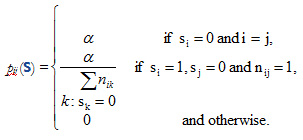
where nij = 1 when individuals i and j know each other and equals 0 when they do not know each other.
In this model, employment status changes as a function of past employment status and the person’s network. The model provides a tool for analyzing effects of social networks on employment dynamics. Calvó-Armengol and Jackson used this model to provide some key explanations for the relationship between employment and network structure (size, diversity).6 Despite the short run conditional negative correlation between employment status and network size, in the long run, network size is positively related to employment across network members. Employment increases with network diversity. Clusters exist in equilibrium as workers with poor networks have higher unemployment rate than their counterparts with better quality networks. The results of this model were also extended to wage dynamics (Calvó-Armengol and Jackson, 2003). The current study is an empirical test in the immigration context of the results implied by the network model, especially on the claim that network structure matters.
In the current paper, the focus is on the empirical evidence of the effect of social capital on the employment probability of immigrants while the relationship between social capital and earnings will be explored later in further work.
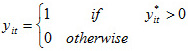
The basic estimating equation used in the research is a logit regression of the probability of employment. An immigrant’s likelihood of getting employment can be thought as an unobserved latent variable y* such that
![]() ,
,
where X is a collection of p independent variables denoted by the vector x’ = (x1, x2, …, xp), which consists of a set of factors, such as immigration category, age, marital status, human capital and social capital, explaining the employment outcome, and ![]() is an error term. I do not observe y*, but rather that the LR (longitudinal respondent) was employed (y = 1) or not (y = 0) at the time of the interview, which takes on values of 0 or 1 according to the following rule:
is an error term. I do not observe y*, but rather that the LR (longitudinal respondent) was employed (y = 1) or not (y = 0) at the time of the interview, which takes on values of 0 or 1 according to the following rule:
![]()
Assuming that ![]() has mean zero and has a standardized logistic distribution with variance
has mean zero and has a standardized logistic distribution with variance ![]() , I get the binary logit model.
, I get the binary logit model.
The estimated models are reduced form. The structural labour supply and labour demand models are not estimated. The analysis extends the human capital earnings function. The basic estimating equation used in the research is a logit regression of the probability of employment on the exogenous variables, covering a range of individual, household and local characteristics:
- Demographic variables: age, marital status, number of children, number of school age children and number of young children at the age between 0 and 4.
- Immigration category: dichotomous variables equal to unity if Skilled Worker Principal Applicants, Skilled Worker Spouses and Dependants, Refugees and Others, with Family Class immigrants as the reference category.
- Region of birth: dichotomous variables equal to unity if born in Asia and Pacific, Central and South America, Europe other than UK and Western Europe, and Africa and Middle East, with North America, UK and Western Europe as the reference category.
- Province of residence: dichotomous variables equal to unity if lived in Atlantic Provinces, Quebec, Prairies Provinces and British Columbia with Ontario as the reference category; A dichotomous variable equal to unity if lived in an area other than the top five CMAs(Census Metropolitan Area) – Toronto, Montreal, Vancouver, Ottawa and Calgary. Inclusion of these variables is to capture the local labour market disparity.
- Ethnic group: dichotomous variables equal to unity if Chinese, South Asian, Black, Filipino, Latin, West Asian and Arab, Other Asian (Southeast Asian, Korean and Japanese), and Other Visible Minority, with White as the reference category.
- Education: dichotomous variables equal to unity if had a master’s degree, college diploma or some university education, some post-secondary education, a high school diploma or less, with a bachelor’s degree as the reference category; A dichotomous variable equal to unity if in school at the time of interview.
- Languages: dichotomous variables equal to unity if has the knowledge of English (speaking fairly well, well, very well and with English as the native language), the knowledge of French (speaking fairly well, well, very well and with French as the native language).
- Experience: length of time in Canada measured in months and a set of dichotomous variables equal to unity if had work experience before immigration, had visited Canada before, had worked in Canada on a work permit before, had studied in Canada on a study permit before, and had an arranged job in Canada when landing.
- Social capital variables: social network indicators specified in Section 4.1. See Table A.1 for details. In addition, spouses’ employment status is likely to determine the attachment to and opportunities in the labour market, so it is included in the explanatory variables and categorized as family factors.
Taking the advantage of the longitudinal feature of the LSIC, this paper presents longitudinal analyses in a panel data model framework in addition to the cross-sectional analyses. The panel data models are taking unobserved individual specific effects into account, which addresses the problems of omitted variables in cross-sectional modelling. The fundamental advantage of a panel data set over a cross section is that it allows modelling differences in behaviour across individuals. In a typical panel, there are a large number of cross-sectional units and only a few periods, like the LSIC micro data. Thus, panel data modelling techniques are focusing on heterogeneity across units rather than time series autocorrelations.
The basic framework for the binary panel data models is a single equation model:
(1) ![]() i=1,…, n, t=1,…, Ti.
i=1,…, n, t=1,…, Ti.
![]()
where i is an index for cross section units and t is an index for time periods. In the current analysis, T = 3. There are p independent variables in Xit, which are observable, either varying with time or not. The unobserved individual effect zi capturing the heterogeneity across individuals that determine the employment probability includes a set of individual specific factors which are unobservable, such as individual difference in personality or ability, health, group or family specific characteristics and cultural attitudes towards labour market participation and so on. If zi contains only a constant term, then the model reduces to an ordinary cross sectional model. If zi contains unobserved variables, pooled cross sectional estimation will provide biased and inconsistent estimates due to omitted variables (i.e. neglected heterogeneity), thus panel models would be more appropriate.
1) Fixed effects logit model
The fixed effects logit model makes the assumption that the unobserved individual effects zi are correlated with Xit, in which case the model is:
(2) ![]() i = 1,…, n; t = 1,…, Ti.
i = 1,…, n; t = 1,…, Ti.
 , so that
(3) ![]()
where F is the cumulative logistic distribution F(a) = exp(a) / (1+exp(a)).
As fitting this model using a full maximum-likelihood approach leads to difficulties, a conditional probability of Yi = ( yi1,…, y iT) conditional on ![]() (Chamberlain 1980). This conditional probability does not involve the time invariant characteristics such as region of birth and ethnic group and the unobserved heterogeneity.
(Chamberlain 1980). This conditional probability does not involve the time invariant characteristics such as region of birth and ethnic group and the unobserved heterogeneity.
The fixed effects model does have some virtues such as that it increases the degree of freedom and the dependence of the explanatory variables is taken into account. However, in logistic regression, fixed effects model would lead to inconsistent estimates due to the so-called incidental parameters problem,7 especially when Ti is fixed and small, like the case in current analysis where Ti = 3. Moreover, fixed effects make inference based on intra-individual rather than inter-individual comparison of employment status so that the fixed effects are also called within-subject effects. Thus only the observations for individuals who switched employment status are used in the estimation, as such a small sample (small Ti) bias is presented in the estimators. Furthermore, by using fixed effects model, I cannot estimate the effects of the variables which do not vary over time but are of interest to me, such as immigration category and ethnic group. Meanwhile, fixed effects model could only be used to deal with balanced panels which have no missing data.
2) Random effects logit model
When assuming that the unobserved individual effects zi in the general model (1) are unrelated to the observed explanatory variables Xit: Cov (Xit, zi) = 0, t = 1, 2,…, T, so that the conditional distribution f (zi | Xit) is independent on Xit, the random effects model is obtained:
(4) ![]() i = 1,…, n; t = 1,…, T i.
i = 1,…, n; t = 1,…, T i.
E (vit | Xit) = 0,
where ![]()
Time invariant variables such as immigration category, ethnic group, region of origin, can be included in the regression as part of Xit which is impossible in the fixed effects model. Under the random effects assumption, the individual effects are strictly uncorrelated with the observed explanatory variables. This view would be appropriate if sampled cross-sectional units are drawn from a large population, which is the case for the longitudinal data set used in this research. The random effects estimator is more efficient than the fixed effects estimator. However, as the assumption places a strong restriction on the distribution of the heterogeneity, the estimates may be inconsistent should the assumption be inappropriate.
3) Generalized Estimating Equations (GEE) population-averaged logit model
An alternative to the random effects assumptions is the generalized estimating equations (GEE) method of Zeger, Liang and Albert (1988). The GEE model for the binary outcome is an extension of the standard logistic regression model from the generalized linear model approach (GLM).
One of the nice features of the GEE model is that the estimate of ![]() is consistent as the assumption of independence of the unobserved individual effects with the explanatory variables is not needed, as required in the random effects model. The population-averaged model does not fully specify the distribution of the population, but rather specifies only a marginal distribution, so that E ( yit | x it) = E ( yit | x i) for all t. The GEE approach relaxes the strict independence assumption of random effects estimation and takes the dependence among units into consideration. The advantage of the GEE over ordinary logistic regression is twofold: when the working correlation structure resembles the true dependence structure, more efficient estimates can be obtained; even if the dependence across periods is not properly modelled, the GEE estimator is still more efficient than pooled logit model. 8
is consistent as the assumption of independence of the unobserved individual effects with the explanatory variables is not needed, as required in the random effects model. The population-averaged model does not fully specify the distribution of the population, but rather specifies only a marginal distribution, so that E ( yit | x it) = E ( yit | x i) for all t. The GEE approach relaxes the strict independence assumption of random effects estimation and takes the dependence among units into consideration. The advantage of the GEE over ordinary logistic regression is twofold: when the working correlation structure resembles the true dependence structure, more efficient estimates can be obtained; even if the dependence across periods is not properly modelled, the GEE estimator is still more efficient than pooled logit model. 8
The GEE models are appropriate when inferences about the population-average are the focus. In this research, the average difference between groups with varied stock of social capital is of most importance, not the difference for any one immigrant. Furthermore, the GEE models could take the survey design into consideration by including the survey weights in the regressions. Thus while the estimates from pooled logit model, fixed effects logit model, random effects logit model and the GEE logit model are contrasted in the results table for a comparison, the GEE logit model is used as the benchmark model for further investigation of time effects and group effects.
Notes
5. Montgomery emphasizes the advantages of network for the employer relative to other hiring channels as it provides a screening against low-ability workers.
6. For detailed proof of propositions, see Calvó-Armengol and Jackson (2004).
7. See Greene (2003) Chapter 21 for a discussion.
8. For a detailed discussion on the comparison of GEE and subject-specific approaches (random effects and fixed effects estimation) for analyzing binary outcomes in longitudinal data, see Neuhaus, Kalbfleisch and Hauck (1991).