
Biological test method for measuring survival of springtails exposed to contaminants in soil: chapter 4
Section 4
Universal Test Procedures
General procedures and conditions described in this section for toxicity tests with springtails apply when testing the toxicity of samples of soil, particulate waste, or chemical, and also apply to their associated reference toxicity tests. More specific procedures for conducting tests with field-collected samples of soil or other similar particulate material (e.g., sludge, de-watered mine tailings, drilling mud residue, compost, biosolids) are provided in Section 5. Guidance and specific procedures for conducting tests with negative control soilor other soils spiked (amended) experimentally with chemical(s) or chemical product(s) are given in Section 6. Specific guidance for conducting tests with boreal and taiga soils has been incorporated throughout this second edition test method document.
All aspects of the test system described in Section 3 must be incorporated into these universal test procedures. Those conditions and procedures described in Section 2 for culturing F. candida, O. folsomi, F. fimetaria and P. minuta in preparation for soil toxicity tests also apply. Summary checklists in Table 2 describe required and recommended conditions and procedures to be universally applied to each test with samples of contaminated or potentially contaminated soil, as well as those for testing specific types of test materials or substances. These could include samples of site soil (including boreal and taiga soils), biosolids (e.g., dredged material, sludge from a sewage treatment plant, composted material or manure) or negative control soil (or other soil, contaminated or clean) spiked in the laboratory with one or more test chemicals or chemical products.
This biological test method measures the effects of exposure to contaminated soil on the survival and reproductive success of springtails. Test organisms must be chosen from four species options (F. candida, O. folsomi, F. fimetaria or P. minuta; see Section 1.2). Test duration is 21 or 28 days, depending on the species chosen (i.e., 21 days for F. fimetaria and P. minuta; and 28 days for F. candidaand O. folsomi),Footnote37 and the test soils are hydrated during the test but not renewed.
This definitive test method was applied and validated by several participating laboratories in three rounds of concurrent tests using F. candida in artificial soil spiked with boric acid (EC, 2007b).Footnote38
Table 2 Checklist of Required and Recommended Conditions and Procedures for Conducting Tests for Effects of Exposure to Contaminated Soil on the Survival and Reproduction of Folsomia candida, Orthonychiurus folsomi, Folsomia fimetaria and Proisotoma minuta
Universal
- for O. folsomi: age-synchronized laboratory cultures; 28 to 31 days after eclosionm
- for F. candida: age-synchronized laboratory cultures; 10 to 12 days after eclosion
- for F. fimetaria: age-synchronized laboratory cultures; 23 to 26 days after eclosion
- for P. minuta: age-synchronized laboratory cultures; 13 to 14 days after eclosion; 14 days recommended
Field-collected Soil
Soil Spiked with Chemical(s) or Chemical Product(s)
4.1 Preparing Test Soils
Each test vessel (see Section 3.2.2) placed within the test facility must be clearly coded or labelled to enable identification of the sample and (if diluted) its concentration. The date and time when the test is started must be recorded, either directly on the labels or on separate data sheets dedicated to the test. The test vessels should be positioned such that observations and measurements can be made easily. Treatments should be positioned randomly within the test facility, and the position of test vessels within the test facility should be changed regularly during the test (i.e., once per week, randomly) (EC, 1997a, b, 2001, 2004a, 2005a, 2013a).
The day that springtails are initially exposed to samples of test materials or substances is designated Day 0. On the day preceding the start of the test (i.e., Day -1), each sample or subsample of test soil or similar particulate material, including negative control soil and, if used, reference soil, should be mixed thoroughlyFootnote39 (see Sections 5.3 and 6.2) to provide a homogeneous mixture consistent in colour, texture and moisture. If field-collected samples of site soil are being prepared for testing, large particles (stones, thatch, sticks, debris) should be removed before mixing, along with any vegetation or macroinvertebrates observed (see Section 5.3). For soils collected as distinct horizons (e.g., boreal and taiga soils), each horizon must be prepared and tested separately. If soils were collected and intended to be tested as consolidated soil samples, they must remain intact for the duration of the test.Footnote40
The quantity of each test soil, or soil horizon mixed as a batch should be enough to establish the replicates of that treatment (see Table 2), plus an additional amount for the physicochemical analyses to be performed (Section 4.6) and a surplus to account for the unused soil that adheres to the sides of the mixing container. The moisture content (%) of each test soil should be known or determined, and adjustments made as necessary by mixing in test water (or, if and as necessary, by dehydrating the sample) until the desired moisture level is achieved (see Sections 5.3 and 6.2). Quantitative measures of the homogeneity of a batch might be made by taking aliquots of the mixture for measurements such as particle size analysis, total organic carbon content (%), organic matter content (%), moisture content (%) and concentration of one or more specific chemicals.
Immediately following the mixing of a batch, 30 gFootnote41 wet weight of test soil should be transferred to each replicate test vessel. The soil added to each test vessel should be smoothed (but not compressed) using a spoon or by gently shaking the vessel back and forth horizontally, or by gently tapping the glass jar ≥ 3 times on the benchtop or with a hand.
For boreal or taiga soils collected as distinct horizons, each horizon must be tested separately in independent definitive tests. For soils to be assessed in multi-concentration tests, each horizon of the test soil is mixed with the same horizon of negative control or reference soil (see Section 5) at the various test concentration (0%, 6.25%, 12.5%, 25%, etc.). In some cases, it may not be possible to collect the same horizons of negative control soil and test soil. For example, negative control soils may be collected in horizons, but this might not be possible at the site of contamination, i.e. more than one horizon of test soil might not be present or horizons may be mixed. In this case, test concentrations are prepared by mixing suitable weights of test soil into the available horizon(s) of negative control soils at the appropriate test concentrations.
For a single-concentration test (e.g., site soil tested at 100% concentration only; a particular concentration of test soil; or a chemical-spiked soil tested at one concentration [e.g., Maximum Label Rate]), a minimum of five replicate test vessels as well as five replicate negative control test vessels must be set up by adding 30 g wet weight of the same batch to each replicate vessel. For site soils, replicates should represent replicate samples (i.e., field replicates) collected individually from a given sample location (see Section 5.1). For a multi-concentration test, a minimum of five replicate test vessels per negative control soil and a minimum of three replicate test vessels per treatment must be set up. In the case of appreciable uncertainty about sample toxicity, a range-finding test might prove worthwhile for selecting, more closely, the concentrations to be used for the definitive test. For a range-finding test, the number of replicates used might be reduced (e.g., two replicates). For any test that is intended to estimate the inhibiting concentration for a specified percent effect (ICp) in a definitive multi-concentration test, at least seven concentrations plus the control treatment(s) must be set up, and more (i.e., ≥ 10 plus controls) are recommended to improve the likelihood of bracketing each endpoint sought.Footnote42
It is recommended that a minimum of two additional test vessels for each treatment (including any control or reference soils used) be included in the test for the purposes of conducting physicochemical analyses on Day 0 and at the end of the test (see Section 4.6).Footnote43
Concentrations should be chosen to span a wide range, including a low concentration that evokes no adverse effects (e.g., similar to that for the negative control treatment), and a high concentration that results in “complete” or severe effects. If the anticipated endpoint is bracketed with a closely spaced series of concentrations, all may turn out to be either too low or too high. To keep the wide range of concentrations, and also obtain the important mid-range effects, it might be necessary to use additional treatments in order to split the selected range more finely. In any case, a consistent geometric series should be used (see Appendix H). See EC (2005b) for additional guidance on selecting test concentrations that apply here.
Following the addition of a measured (30 g wet wt) aliquot of test soil to each test vessel, lids (Section 3.2.2) should be placed onto the test vessels and closed tightly to minimize loss of moisture. The test vessels should be held overnight under specified test temperature and lighting conditions (Section 4.3), for chemical equilibration (e.g., of chemical-spiked soil or site soil diluted with control soil) of the test soils.
4.2 Beginning the Test
Test organisms are transferred to each test vessel the day after the soil is prepared (i.e., Day 0 of the toxicity test). A number of test organisms in excess of those required for the test should be available from a group of age-synchronized culture vessels established to yield the appropriate number of organisms required for a test (Section 2.3.8).
For tests using O. folsomi, 28- to 31-day-old individuals, from age-synchronized cultures (see Section 2.3.8 for information on the age synchronization of all species) must be used. Fifteen individuals (10 females, larger with round abdomens, and 5 males, smaller and more slender) are transferred into each test vessel.Footnote44 For tests using F. candida, 10- to 12-day-old juveniles from age-synchronized cultures must be used. Ten individuals are gently transferred from the age-synchronized cultures into each test vessel. For tests using F. fimetaria, 23- to 26-day-old organisms from age-synchronized cultures must be used, and 20 individuals (10 females, larger with round abdomens, and 10 males, more slender and half the size of the females) are transferred into each test vessel.Footnote45 For tests using P. minuta, 13- to 14-day-old organisms (recommend using only 14-day-old organisms) from age-synchronized cultures must be used, and 10 individuals (5 females, larger with round abdomens, and 5 males, smaller and more slender) are transferred into each test vessel.Footnote46
For all four test species, organisms can be gently transferred from the age-synchronized culture to a piece of folded stiff cardboard (8.5 × 11 in. paper folded in half)Footnote47 or a weigh boat (previously washed and dried to remove a waxy film that coats the weigh boats), using a fine, moistened paintbrush and a probe or a low- suction exhaustor system (see Section 2.3.7). The use of a low-suction vacuum aspiration system in conjunction with a dissecting microscope is highly recommended in order to effectively separate male and female P. minuta for use in toxicity tests (see Appendix I).Footnote48 For F. candida, organisms can be transferred by tapping the individuals directly from the age- synchronized culture onto the piece of black cardboard. The latter method enables the transfer of the required amount of individuals with the least amount of loss due to the natural springing tendency of the F. candida.
For O. folsomi, F. fimetaria and P. minuta, the age-synchronized cultures should be carefully examined to determine which organisms are male and which are female. Organisms should be gently picked up one at a time until the desired number of males and females (i.e., 10 females and 5 males for O. folsomi; 10 females and 10 males for F. fimetaria; and 5 females and 5 males for P. minuta) has been collected. Final observation of springtails should be made to confirm that the correct number and sex ratio of organisms has been selected, and that their appearance is normal (i.e., organisms chosen should appear healthy and active, demonstrating movement, lack of visible defects or damaged bodies, and should be similar in colourationFootnote49). Any atypical Collembola should be discarded. Thereafter, the organisms should be carefully transferred to the surface of the soil in a test vessel, by gently tapping the cardboard or the weigh boat over the test vessel. The group of springtails transferred to each test vessel should be random across the replicates and treatments.
4.3 Test Conditions
- This is a 21- or 28-day soil toxicity test during which the soil in each test vessel is not renewed. The test duration for F. fimetaria and P. minuta is 21 days, and for F. candida and O. folsomi, the test duration is 28 days.
- The test vessel is a 100- to 125-mL wide-mouthed glass jar; its content (i.e., 30 g wet wt of test soil) is covered (Section 3.2.2).
- For a single-concentration test, at least five replicate test vessels must be set up for each test soil (i.e., each treatment). For a multi- concentration test, a minimum of three replicate test vessels per test concentration and five replicate test vessels per control soil must be set up.
- For multi-concentration tests for all four species, at least seven concentrations plus the appropriate control treatment(s) must be used, and more concentrations (i.e., ≥ 10 plus controls) are recommended.
- The test must be conducted at a daily mean temperature of 20 ± 2°C. Additionally, the instantaneous temperature must always be 20 ± 3°C.
- Test vessels must be illuminated with a fixed daily photoperiod (e.g., 16-h light and 8-h dark, or 12-h light and 12-h dark), and should use incandescent or fluorescent lights. Light intensity adjacent to the surface of the soil in each test vessel should be 400−800 lux, and must be at least 400 lux as a minimum. This range is equivalent to a quantal flux of 5.6−11.2 μmol/(m2 . s) for cool-white fluorescent, 6.4−12.8 μmol/(m2 . s) for full-spectrum fluorescent, or 7.6−15.2 μmol/(m2 . s) for incandescent.
4.4 Criteria for a Valid Test
For the results of this biological test method to be considered valid, each of the following criteria, specific to each species must be achieved:Footnote50
For Folsomia candida:
- the mean survival rate for adult springtails held in negative control soil for 28 days must be ≥ 70% for tests conducted in natural soil, and ≥ 80% for tests conducted in artificial soil, at the end of the test
- the reproduction rate for the adult springtails in negative control soil for 28 days must average ≥ 100 live juveniles per control vessel
For Orthonychiurus folsomi:
- the mean survival rate for the adults held in negative control soil for 28 days must be ≥ 70% at the end of the test
- the reproduction rate for the adult springtails in negative control soil for 28 days must average ≥ 100 live juveniles per control vessel
For Folsomia fimetaria:
- the mean survival rate for adult springtails held in negative control soil for 21 days must be ≥ 70% at the end of the test
- the reproduction rate for the adult springtails in negative control soil for 21 days must average ≥ 100 live juveniles per control vessel
For Proisotoma minuta:
- the mean survival rate for the adults held in negative control soil for 21 days must be ≥ 60% for tests conducted in natural soil, and ≥ 70% for tests conducted in artificial soil, at the end of the test
- the reproduction rate for the adult springtails in negative control soil for 21 days must average ≥ 100 live juveniles per control vessel
4.5 Food and Feeding
During a toxicity test, O. folsomi in each test vessel are fed ~5 mg of granulated dry yeast, every seven days, starting at Day 0 and continuing until and including Day 21. For tests using F. fimetaria, ~10 mg of dry yeast is added to each test vessel on Days 0 and 14, and for F. candida, ~10 mg of dry yeast is added to each test vessel on Day 0 and ~20 mg on Day 14. P. minuta are fed ~10 mg of granulated yeast every seven days, starting at Day 0 and continuing until and including Day 14. The type of yeast used is a dried, activated yeast (e.g., Fleischman’s™) and is prepared by distributing the yeast uniformly over the surface of the moist test soil, or over the dry soil and then spraying the soil three times to activate the yeast and moisten the soil. It is important that the same amount of yeast is available to organisms in each test vessel. If, when adding yeast to a test vessel, it is noticed that the yeast from a previous feeding period has not been consumed, the unconsumed yeast should not be removed and no further yeast is added to the test vessel at that time.Footnote51
4.6 Observations and Measurements During the Test
The biological endpoints for the test are the number of live adult springtails and the number of progenyproduced in each test vessel at the end of the test (Day 21 for F. fimetaria and P. minuta; and Day 28 for F. candida and O. folsomi). The condition, appearance and number of live springtails transferred to each test vessel on Day 0 must be observed and recorded. The lid must be removed from each test vessel for the purpose of aeration at least once/week or more frequently (i.e., ≥ 2 times per week) as necessary, or as the test progresses and the number of organisms per test vessel increases.Footnote52 Observations and records should be made at this time regarding any excessive growth of bacteria or fungi, any feeding activity, and the presence and quantity of any uneaten food.
Air temperature in the test facility (Section 4.3) must be measured daily (e.g., using a maximum/minimum thermometer) or continuously (e.g., using a continuous chart recorder).
The contents of each replicate vessel should be examined weekly for apparent “wetness.” If, for any treatment, the soil appears to be too dry at any time during the test, all replicates representing that treatment should be examined. The surface of the soil in each test vessel that appears to be too dry should then be moistened with test water using a fine-spray mister that disperses about 1 mL of water per spray.Footnote53
Alternatively, test vessels can be weighed to determine moisture loss (ISO, 1999). All vessels can be weighed at the beginning of the test. The weight of each test vessel can then be checked every two weeks and test water added to compensate for weight loss (i.e., due to water loss), if the loss is > 2% of the initial water content (ISO, 1999). For a large number of test vessels, the average amount of water lost can be calculated by weighing a random sample of 5 or 10 test vessels. This amount of test water can then be added to all of the test vessels.
The pH and moisture content of the test soil or soil horizon representing each treatment (including the negative control soil and, if used, reference soil) must be measured and recorded at the beginning and end of the test. Additionally, it is recommended that conductivity be measured at the beginning and end of the test in instances where the test soil is anticipated to have a high salt content. The initial (Day 0) measurements should be made using a composite sample made up of subsamples of each batch of test soil or soil horizon used to set up replicates of a particular treatment (see Section 4.3).Footnote54 The final (i.e., Day 21 or Day 28, depending on the species used) measurements should be made using additional replicates set up for each treatment (see Section 4.1) that are analyzed at the end of the test.
Soil pH should be measured using a calcium chloride (CaCl2) slurry method (modified from Hendershot et al., 1993).Footnote55 For these analyses, 4 g of hydrated soilFootnote56 is placed into a 30-mL glass beaker (~3 cm in diameter and ~7 cm high) with 20 mL of 0.01 M CaCl2.Footnote57 The suspension should be stirred intermittently for 30 min (e.g., once every 6 min). The slurry should then be left undisturbed for ~1 h. Thereafter, a pH probe is immersed into the supernatant, and when the meter reading is constant, the pH is recorded.
The moisture content of each test soil or soil horizon is measured by placing a 3−5 g subsample of each test soil or horizon into a pre-weighed aluminum weighing pan, and measuring and recording the wet weight of the subsample. Each subsample should then be placed into a drying oven at 105°C until a constant weight is achieved; this usually requires a minimum of 24 hours. The dry weight of each subsample should then be measured and recorded. Soil moisture content must be calculated (on a dry-weight basis) by expressing the moisture content as a percentage of the soil dry weight:
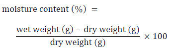
Long description
The moisture content of soil is determined on a dry weight basis by subtracting the dried weight of a soil sample from the pre-dried weight of the same sample. This result is then divided by the samples dry weight and multiplied by 100.
It is important that the calculation of moisture content (%) be based on dry weight (not on wet weight), since the results of these calculations are used with calculations of water-holding capacity (also calculated based on dry weight) to express the optimal moisture content in test soils (see Section 5.3).
Depending on the nature of the test and the study design, concentrations of chemical(s) or chemical product(s) of concern might be measured for test soils or selected concentrations thereof, at the beginning and end of the test. For a test using a sample of field-collected site soil, the chemical(s) or chemical product(s) measured will depend on the contaminant(s) of concern (see Section 5.5). For a multi-concentration test with chemical-spiked soil, such measurements should be made for the high, medium and low concentrations tested, as a minimum (see Section 6.3). Aliquots for these analyses should be taken for each soil or soil horizon as described previously for pH and moisture content; analyses should be according to proven and recognized (e.g., SPAC, 1992; Carter, 1993) analytical techniques.
4.7 Ending the Test
The test is terminated after 21 days of exposure for F. fimetaria and P. minuta, and 28 days of exposure for F. candida and O. folsomi. At that time, the number of live adult springtails and the number of live progeny in each test vessel must be observed and recorded. Before opening a test vessel, the lid should be tapped (e.g., three times) to dislodge any individuals from the underside. Two different options are recommended for extracting the Collembola from the test soil: (i) the flotation method, and (ii) the heat extraction method.Footnote58
For the flotation method, test water is added to the test vessel, to about 2 cm above the surface of the soil, and the slurry is stirred with a glass stir rod. The Collembola, both adult and progeny produced during the test, float to the surface of the water;Footnote59 then, they can either be removed with a moistened paint brush and counted, or the supernatant can be poured into a wide Petri dish. The Collembola are distributed over the surface of the water in the Petri plate and can be easily counted systematically and their numbers recorded.Footnote60 Once the individuals have been counted, the water in the Petri dish is discarded. Water is then added again to the test vessel, the slurry is stirred vigorously to break up soil particles and dislodge Collembola, and the individuals enumerated by pouring the water (and the suspended or floating Collembola) into the Petri dish where they are counted and recorded. These procedures are repeated until Collembola no longer float to the surface when water is added to the soil remaining in the test vessel.
Alternatively, the soil from each test vessel is poured into a 500 mL glass beaker (9-cm diam.) to which 150 mL of water is added. The test vessel is rinsed with water, which is then added to the slurry in the beaker. After gentle stirring with a spatula, approximately 250 mL of water and blue bromophenol (or any other dark- coloured dye that is not toxic to the Collembola) is added (the latter to improve the contrast between the whitish Collembola and the water). The mixture is stirred thoroughly. The beakers are then filled with water to 500 mL, and the number of juveniles and adults are either counted manually on the surface of the water, or by taking a digital photograph or colour slide of the water surface. The image is then transferred to a computer screen or a paper hardcopy, or projected using a table projector for enumeration of adults and juveniles. If the test vessel contains a large number of organisms, the Collembola tend to clump together, thereby making it difficult to count individuals. In this case, the organisms can be poured out or split into several (e.g., three) aliquots in preparation for photography. The individuals in each digital image can then be more easily counted and the results of all of the aliquots tallied for a final vessel count. There are a number of other methods that can be used for enumerating adult and juvenile Collembola at the end of the test, including the use of image analysis software and other image processing devices (Krogh et al., 1998). If springtails are enumerated using image analysis or any other automated counting method, the method must be previously verified using some form of a manual count to ensure that the numbers being produced by the automated system are accurate.
The heat extraction method described by Wiles and Krogh (1998) and OECD (2009) is based on principles of MacFayden and of Petersen, and involves a controlled temperature gradient extractor, where the organisms are collected over a 48-h period.Footnote61 Becker-van Slooten et al. (2005) developed a simpler and more cost-effective heat extraction technique. This method, which was then further refined by Environment Canada (2006b) using equipment available in Canada, is recommended herein as an alternative to the flotation method for the extraction of springtails from test soil. The heat comes from a lamp fitted with a 60- or 100-watt lightbulb, and is regulated by the distance of the lightbulb from the surface of the soil in the heat extraction unit.Footnote62 One heat extraction unit should be prepared for each test vessel. At test termination, the soil from each test vessel is transferred into a heat extraction unit.Footnote63
The soil surface is smoothed out evenly over the mesh, using a spoon or a scoopula. The heat extraction units are placed underneath the lamps, limiting the number of units per lamp to no more than five or six, so that the heat and light are kept consistent for each unit. The bottom of the lightbulb is adjusted to 30 cm above the top of the soil and a thermometer (e.g., electronic thermometer) is set up within one of the units to monitor temperature changes throughout the extraction. The temperature should be recorded every 12 hours or at the beginning and end of each work day (i.e., 9:00 a.m. and 5:00 p.m.). For tests with O. folsomi and F. fimetaria, the lamp height does not need any adjustment, and the temperature should reach ~32°C after 48 hours. For F. candida and P. minuta, the lamp should be lowered so that the bottom of the lightbulb is 25 cm above the top of the soil after 24 hours of the extraction, and the temperature reaches ~36°C after 48 h. At the end of the extraction period (i.e., 48 h), the lamps should be turned off and the Parafilm® removed. The organisms that have dropped down through the mesh to the plaster of Paris substrate can be counted immediately, either manually or through image analysis, as previously described, or they can be preserved (e.g., in 70% alcohol) for enumeration at a later date.
Laboratories that are inexperienced with the heat extraction procedure described must initially establish and document the efficiency of their heat extraction system (i.e., demonstrate and record data that show that a significant number of test organisms are not being left in the soil following heat extraction). This can be demonstrated by further processing the heat-extracted soil for test organisms using the flotation method as a check on the efficiency of the heat-extraction technique. This method requirement is the direct result of problems identified during the method interlaboratory studies. The heat extraction process is considered acceptable if < 5% of the total number of test organisms extracted from the soil are removed using flotation, following heat extraction. Once laboratory personnel are experienced with heat extraction and have demonstrated the efficiency of their system, they should continue monitoring the efficiency periodically.
In general, adults can be easily distinguished from juveniles by their significantly greater size; however, male F. fimetaria and P. minutaFootnote64 can be mistaken for juveniles because their sizes are similar. Experience with these species will improve the ability to distinguish males from progeny (Stämpfli et al., 2005; C. Fraser, personal communication, Soil Toxicology Laboratory, Environmental Science and Technology Centre, Ottawa, ON, 2013). The number of adult springtails and the number of progeny, alive or dead, must be counted and recorded. Live O. folsomi, F. candida/fimetaria are opaque/white, mobile on the water’s surface, and are often curled up, taking five seconds to one minute to uncurl. Live P. minuta are dark grey in colour, and like the other test species should be observed for short period of time to detect movement or a lack thereof. A springtail is considered dead if there is complete cessation of movement of any type of body part including legs, abdomen, head and antennae. Dead Collembola appear transparent and stretched out or elongated with legs fully extended, and can be distinguished from molted carapaces, as the latter are translucent and collapsed. Since the bodies of dead adult Collembola decompose rapidly and are usually not seen, any missing Collembola are considered as dead. Live juveniles must be distinguished from the adults and counted separately. If dead juveniles are observed, they should be noted.
Test vessels, irrespective of concentration levels, should be processed in a random manner since the perception of size tends to change over time, and discrimination between adults and juveniles and counting may become more or less accurate. Extra replicates of each test soil (including the negative control soil and, if included in the test, reference soil) set up for the purpose of physicochemical analyses should be analyzed to determine the pH and moisture content at the end of the test (Section 4.6). Analyses for other chemical constituents (i.e., concentrations of contaminants) should also be made at this time using additional replicates prepared for each test soil (Section 4.6).
4.8 Test Endpoints and Calculations
For each test, the percent survival for all replicate groups of adult springtails in each test vessel at the end of the test (i.e., Day 21 for F. fimetaria and P. minuta, and Day 28 for F. candida and O. folsomi) must be calculated and reported. The mean (± SD) percent survival for all springtails exposed to each concentration must also be calculated and reported for the end of the test, using the survival data determined from all treatment replicates (e.g., the mean of the replicates within each treatment).
The reproductive endpoint for this test is based on the number of surviving progeny produced in each replicate and each treatment during the test period. A significant reduction in this number is considered indicative of an adverse toxic effect of the treatment on the reproductive success of the adult Collembola. The mean (± SD) value for number of surviving progeny in the test soil on Day 21 for F. fimetariaand P. minuta, and Day 28 for F. candidaand O. folsomi, is determined for each treatment including reference and negative control soils.
The two most common possibilities for a typical test design involve:
- Multiple sampling locations, in which responses at one or more test site sampling location(s) are compared with those at a reference site sampling location,Footnote65 with other test sampling locations, or with the control soil (i.e., single-concentration test). Hypothesis testing is frequently used in the statistical assessment, and the common outcome is that a response at a sampling location is either “different” or “not different” from another sampling location.
- Multiple concentrations of a test soil, achieved by mixing a test soil with reference or control soil (Section 5.3), or by spiking a soil with various concentrations of a chemical or chemical product (Section 6.2). For a multi-concentration test, the 21- or 28-day LC50 for survival and ICp for reproductive inhibition must be calculated and reported (data permitting).Footnote66
In a scenario where there are multiple sampling locations, an understanding of the strengths of various study designs is critical for the successful application of statistical tests. The study objectives should be clearly defined before data are collected, with an appreciation both for the power (ability to detect an effect) of the test design and the ease of interpretation of the results. In general, it is advantageous to limit the number of comparisons made, and this is typically done by choosing a test design and statistical tests that compare test sampling locations with a reference sampling location. Further gains in power can be made if a gradient can be assumed (i.e., samples collected in sequential order away from the point source; see Section P.4 in EC, 2005b). In some cases, study objectives and test design may not have been given adequate attention before the collection of the data, and to compensate, investigators will perform a comparison among all possible sampling locations, maximizing the number of comparisons made. This is strongly discouraged, particularly when large numbers of sampling locations are involved, because (1) undesirable effects on Type I and Type II error rates may occur; (2) interpretation of results is often more difficult; and (3) unwarranted focus may be given to particular comparisons after data have been collected.Footnote67 Detailed statistical guidance on hypothesis testing for the number of live offspring at test end is provided in Section 5.6.
Environment Canada (2005b) provides direction and advice for calculating LCp and ICp endpoints, which should be followed; Sections 4.8.1 and 4.8.2 give further guidance in this regard. Initially, regression techniques (see Section 4.8.2.1) must be applied to multi- concentration data intended for calculation of an ICp.Footnote68 In the event that the data do not lend themselves to calculating the 21- or 28-day ICps for the reproductive inhibition using the appropriate regression analysis, linear interpolation of these data using the program ICPIN should be applied in an attempt to derive an ICp (see Section 4.8.2.2).
An initial plot of the raw data (percent mortality and number of surviving progeny) against the logarithm of concentration is highly recommended, both for a visual representation of the data, and to check for reasonable results by comparison with later statistical computations. Any major disparity between the approximate graphic LC50 or ICp and the subsequent computer-derived LC50 or ICp must be resolved. The graph would also show whether a logical relationship was obtained between log concentrations (or, in certain instances, concentration) and effect, a desirable feature of a valid test (EC, 2005b).
4.8.1 LC50
When a multi-concentration test with soil mixtures is conducted, the quantal mortality data for a specific period of exposure must be used to calculate (data permitting) the appropriate median lethal concentration (LC50), together with its 95% confidence limits. For F. fimetaria and P. minuta, the 21-day LC50 for the adult (first generation) springtails must be calculated and reported, data permitting; and for F. candida and O. folsomi, the 28-day LC50 for the adult (first generation) springtails must be calculated and reported, data permittingFootnote69 (see Section 4.8). To estimate an LC50, mortality data at the specified period of exposure are combined for all replicates at each concentration.
The guidance provided by Environment Canada (2005b) on choosing statistical test methods to be applied to quantal (e.g., LC50) data should be consulted when choosing the statistical test to be applied to such data for toxicity tests using springtails.
The optimization of the calculation of the LC50 and its 95% confidence intervals is based on the number of partial effects observed (EC, 2005b). In brief, probit and/or logit regression is the preferred method if two partial effects are observed, the Spearman-Kärber method is preferred if only one partial effect is observed, and the binomial method is used if no partial effects are observed, and as a general “default” method.
4.8.2 ICp
When a multi-concentration test for effects of exposure of springtails to field-collected or spiked-soil mixtures is conducted, the quantitative data representing reproductive inhibition must be used to calculate the ICp (see introductory paragraphs of Section 4.8, and Section 6.2). The ICp is a quantitative estimate of the concentration causing a fixed percent reduction in the mean number of progeny produced by the adult springtails during the test.
The ICp is calculated as a specified percent reduction (e.g., the IC25 and/or IC20, which represent 25% and 20% inhibition, respectively). The desired value of p is selected by the investigator, and 25% or 20% is currently favoured. Any ICp that is calculated and reported must include the 95% confidence limits.
In the analyses of reproductive performance, the number of progeny produced in each replicate is used to calculate the average number of surviving progeny produced per treatment (concentration) in relation to the average number produced in the negative control replicates. A value of zero is assigned for the number of juveniles in a replicate, if all of the adult springtails in that replicate died before producing progeny. If any of the adult Collembola died during the test, after producing young, the number of progeny produced is still to be used in the analyses. If there are no surviving progeny in a replicate (test vessel), it contributes a value of zero to the calculation used to obtain the average number of survivors for that treatment (concentration). If there are no surviving progeny in all replicates at a given concentration, that concentration is still included in the analysis, using an average value of zero juveniles.
As previously indicated, an ICp for mean number of surviving progeny produced in each treatment must be calculated and reported (data permitting) upon completion of a 21-day multi- concentration test with F. fimetaria and P. minuta, and a 28-day multi-concentration test with F. candida and O. folsomi. These calculations must be made using the appropriate linear or nonlinear regression analyses (see the following Section 4.8.2.1). If, however, regression analyses fail to provide meaningful ICps for the mean number of live progeny produced, the ICPIN analyses described in Section 4.8.2.2 should be applied to the corresponding data.
4.8.2.1 Use of regression analysis.
Upon completion of a definitive 21-day (for F. fimetaria and P. minuta),or 28-day (for F. candida and O. folsomi) multi-concentration test, an ICp (including its 95% confidence limits) for the mean number of surviving progeny produced in each treatment must be calculated using regression analysis, provided that the assumptions below are met. A number of models are available to assess reproduction data (using quantitative statistical tests) via regression analysis. The proposed models for application consist of one linear model, and the following four nonlinear regression models: exponential, Gompertz, logistic and logistic adjusted to accommodate hormesisFootnote70 (see Section 6.5.8 in EC, 2005b). Use of regression techniques requires that the data meet assumptions of normality and homoscedasticity. The reader is strongly advised to consult EC (2005b) for additional guidance on the general application of linear and non-linear regression for the analysis of quantitative toxicity data.Footnote 71
The general process for the statistical analysis and selection of the most appropriate regression model (linear or non-linear) for quantitative toxicity data is outlined in Figure 7. The selection process begins with an examination of a scatter plot or line graph of the test data to determine the shape of the concentration-response curve. The shape of the curve is then compared to available models so that one or more appropriate model(s) that best suits the data is (are) selected for further examination (refer to Figure O.1, Appendix O, in EC, 2005b for an example of five potential models).
Once the appropriate model(s) is (are) selected for further consideration, assumptions of normality and homoscedasticity of the residuals are assessed. If the regression procedure for one or more of the examined models meets the assumptions, the data (and regression) are examined for the presence of outliers. If an outlier has been observed, the test records and experimental conditions should be scrutinized for human error. If there are one or more outliers present, the analysis should be performed with and without the outlier(s), and the results of the analyses compared to examine the effect of the outlier(s) on the regression. Thereafter, a decision must be made as to whether the outlier(s) should be removed from the final analysis. The decision should take into consideration natural biological variation, and biological reasons that might have caused the apparent anomaly. Additional guidance on the presence of outliers and unusual observations is provided in Section 10.2 of EC (2005b). If there are no outliers present or none are removed from the final analysis, the model that demonstrates the smallest residual mean square error is selected as the model of best choice.Footnote72 Additional guidance from a statistician familiar with dealing with outlier data is also advised.
Figure 7 The General Process for the Statistical Analysis and Selection of the Most Appropriate Model for Quantitative Toxicity Data (adapted and modified from Stephenson et al., 2000b)
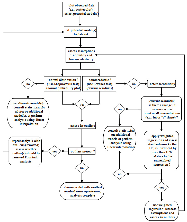
Long description
The general process for the statistical analysis and selection of the most appropriate model for quantitative toxicity data This figure depicts a decision tree designed to aid the reader in choosing the correct statistical model to analyze their data. The tree asks the reader to select potential models by examining a plot of the data. These models are then fit to the data and accessed for normality and homoscedasticity. If both of these assumptions are met, the reader is asked to assess for outliers. In the absence of outliers the model with the smallest residual mean square error is the most appropriate. If outliers are present, one should repeat the analysis with them removed and then make a judgment concerning their inclusion in the final analysis. If it is found that the data does not fit a normal distribution then the reader can choose to: use alternative models, use a linear interpolation, or consult a statistician. In the case that the data is heteroscedastic then the reader should examine the residuals for a change in variance across concentrations. If there is a change in variance, and the standard error for the ICp is reduced by more than 10% when a weighted regression is applied, then the assumption of homoscedasticity should be reassessed using this weighted regression. If there is no change in variance across concentrations, or a weighted regression does not reduce the standard error of the ICp by more than 10%, then a linear interpolation should be employed or a statistician should be consulted.
Normality should be assessed using the Shapiro-Wilk’s test as described in EC (2005b). A normal probability plot of the residuals may also be used during the regression procedure, but is not recommended as a stand-alone test for normality, as the detection of a “normal” or “non-normal” distribution is dependent upon the subjective assessment of the user. If the data are not normally distributed, then the user is advised to try another model, consult a statistician for further guidance on model selection, or perform the less-desirable linear interpolation (using ICPIN, see Section 4.8.2.2) method of analysis.
Homoscedasticity of the residuals should be assessed using Levene’s test as described in EC (2005b), and by examining the graphs of the residuals against the actual and predicted (estimated) values. Levene’s test provides a definite indication of whether the data are homogeneous (e.g., as in Figure O.2A of Appendix O in EC, 2005b) or not. If the data (as indicated by Levene’s test) are heteroscedastic (i.e., not homogeneous), then the graphs of the residuals should be examined. If there is a significant change in the variance and the graphs of the residuals produce a distinct fan or “V” pattern (refer to Figure O.2B, Appendix O in EC, 2005b for an example), then the data analysis should be repeated using weighted regression. Traditionally, the data have been weighted by dividing by the inverse of the variance; however, other options are available. Before choosing the weighted regression, the standard error of the ICp is compared to that derived from the unweighted regression. If there is a difference of greater than 10% between the two standard errors,Footnote73 then the weighted regression is selected as the regression of best choice. However, if there is less than a 10% difference in the standard error between the weighted and unweighted regressions, then the user should consult a statistician for the application of additional models, given the test data, or the data could be re-analyzed using the less-desirable linear interpolation (using ICPIN, see Section 4.8.2.2) method of analysis. This comparison between weighted and unweighted regression is completed for each of the selected models while proceeding through the process of final model selection (i.e., model and regression of best choice). Some non-divergent patterns might be indicative of an inappropriate or incorrect model (refer to Figure O.2C, Appendix O in EC, 2005b, for an example), and the user is again urged to consult a statistician for further guidance on the application of additional models.
Endpoints generated by regression analysis must be bracketed by test concentrations; extrapolation of endpoints beyond the highest test concentration is not an acceptable practice (EC, 2005b).
4.8.2.2 Linear interpolation using ICPIN.
If regression analyses of the endpoint data (see preceding Section 4.8.2.1) fail to provide an acceptable ICp for reproductive inhibition (i.e., assumptions of normality and homoscedasticity cannot be met), linear interpolation using the computer program called ICPIN should be applied. This program (Norberg-King, 1993; USEPA, 1995, 2002) is not proprietary, is available from the USEPA, and is included in most computer software for environmental toxicology, including TOXSTAT (1996). The original instructions for ICPIN from the USEPA are clearly written and make the program easy to use (Norberg-King, 1993).Footnote74 An earlier version was called BOOTSTRP.
Analysis by ICPIN does not require equal numbers of replicates in different concentrations. The ICp is estimated by smoothing of the data as necessary, then using the two data-points adjacent to the selected ICp (USEPA, 1995, Appendix L; USEPA, 2002, Appendix M). The ICp cannot be calculated unless there are test concentrations both lower and higher than the ICp; both those concentrations should have an effect reasonably close to the selected value of p, preferably within 20% of it. At present, the computer program does not use a logarithmic scale of concentration, and so Canadian users of the program must enter the concentrations as logarithms. Some commercial computer packages have the logarithmic transformation as a general option, but investigators should make sure that it is actually retained when proceeding to ICPIN. ICPIN estimates confidence limits by a special “bootstrap” technique because usual methods would not be valid. Bootstrapping performs many resamplings from the original measurements. The investigator must specify the number of resamplings, which can range from 80 to 1000. At least 400 is recommended here, and 1000 would be beneficial.Footnote75
If there are several adjacent high concentrations with no surviving juveniles, only the lowest of that string of concentrations should be used in analysis (i.e., the concentration closest to the middle of the series of concentrations used in the test). Normally, there is no particular benefit to including the additional concentrations, because they offer nothing to the analysis (i.e., the data consist only of zero progeny).
Besides determining and reporting the computer-derived ICps for Collembola reproduction at test end, a graph of percent reduction in number of live progeny produced should be plotted against the logarithm of concentration, to check the mathematical estimations and to provide visual assessments of the nature of the data (EC, 2005b).
If the ICPIN program is used when there is a hormetic effect, an inherent smoothing procedure could change the control value and bias the estimate of ICP. Accordingly, before statistical analysis, hormetic values at low concentration(s) should be arbitrarily replaced by the control value. This is considered a temporary expedient until a superior approach is established (see Option 4, Section 10.3.3 in EC 2005b). The correction is applied for any test concentration in which the average effect (i.e., the geometric average of the replicate means) is higher (“better”) than the average for the control. To apply this correction, replace the observed mean numbers of progeny of the replicates in the hormetic concentration(s), with the means of replicates in the control. The geometric average for that/those concentration(s) will then be the same as that for the control.
4.9 Tests with a Reference Toxicant
Table 14 of Appendix F summarizes the guidance for performing reference toxicity tests given in other documents describing procedures and conditions for conducting tests of soil toxicity using springtails. Described herein are the procedures and conditions to be followed when performing reference toxicity tests in conjunction with a 21-day (for F. fimetaria and P. minuta), or 28-day (for F. candida and O. folsomi) test of soil toxicity using springtails. These procedures also apply to tests for assessing the acceptability and suitability of cultures of F. fimetaria, F. candida, O. folsomi or P. minuta to be used in soil toxicity tests. They should be applied to assess intralaboratory precision when a laboratory is inexperienced with the biological test method defined in this document and during initial test setup (see Sections 2.3.1, 2.3.9).
The routine use of a reference toxicant is necessary to assess, under standardized test conditions, the relative sensitivity of a portion of the population of adult springtails within a particular culture (Section 2.3.9) from which test organisms are selected for use in one or more definitive soil toxicity tests. Tests with a reference toxicant also serve to demonstrate the precision and reliability of data produced by the laboratory personnel for that reference toxicant, under standardized test conditions. A reference toxicity test, conducted according to the procedures and conditions described herein, must be performed according to one of the following regimes:
- at least once every two monthsFootnote76 using organisms taken from the population of springtails that is being cultured for use in the definitive test(s) (Section 2.3)
- at the same time as the definitive soil toxicity test(s), using organisms taken from the same population as those used for the definitive test(s) (see Sections 2.3.8 and 2.3.9)
A laboratory that cultures springtails and frequently performs soil toxicity tests using these organisms might choose to monitor the sensitivity of their culture(s) to one or more reference toxicants on a routine (e.g., every two months) schedule, while including a reference toxicity test using a portion of the springtails used to start a definitive soil toxicity test. Alternatively, a laboratory might choose to monitor the sensitivity of their culture(s) to a reference toxicant less frequently (e.g., two or three times a year), and perform a reference toxicity test at the time that each definitive soil toxicity test is performed.
Each reference toxicity test performed in conjunction with a definitive test for soil toxicity must be conducted as a static multi-concentration acute lethality test. The reference toxicity test must be 7 days in length for O. folsomi and F. fimetaria, and 14 days in length for F. candidaFootnote77 and P. minuta. The test conditions and procedures described herein for performing an acute (7- or 14-day) lethality test must be applied to each reference toxicity test. Additional conditions and procedures described in Section 4 for performing a multi-concentration test with samples of test soil apply equally to each reference toxicity test. Procedures given in Section 6 for the preparation and testing of chemicals spiked in negative control soil also apply here, and should be referred to for further information. Environment Canada’s guidance document on using negative control sediment spiked with a reference toxicant (EC, 1995) provides useful information that is also applicable when performing reference toxicity tests with negative control soil spiked with a reference toxicant.
The reference toxicity test should be performed using 100- to 125-mL glass jars as test vessels (Section 3.2.2) and a 30-g wet wt aliquot of test soil representing each treatment (concentration) in each test vessel. The number of replicate test vessels per reference toxicant concentration must be ≥ 3; and ≥ 5 for negative control soil. The number of springtails per test vessel is 10 for F. candida and P. minuta (i.e., 5 males and 5 females for P. minuta) as described in Section 4.2. For reference toxicity tests using O. folsomi, and F. fimetaria, 10 organisms (5 males and 5 females) per test vessel are also required; however, this differs from the definitive test design that requires 15 organisms (5 males and 10 females) per test vessel for O. folsomi and 20 organisms (10 males and 10 females) per test vessel for F. fimetaria (see Section 4.2).
Procedures for starting and ending a reference toxicity test should be consistent with those described in Sections 4.2 and 4.7 with the exception of the shorter (7 days for O. folsomi, and F. fimetaria, and 14 days for F. candida and P. minuta) test duration. Test conditions described in Section 4.3 apply. Test observations and measurements given in Section 4.6 should be followed.
To be valid, the mean adult survival rate at the end of the test (Day 7 or Day 14) for springtails held in the aliquots of negative control soil used in a particular reference toxicity test must be at least 80% for F. candida, F. fimetaria and O. folsomi; and at least 70% for P. minuta. Test endpoints to be calculated and reported include the mean percent survival in each treatment at test end (Day 7 or Day 14), and the 7-day or 14-day LC50 (including its 95% confidence limits), depending on the species used. Results for a reference toxicity test should be expressed as mg reference chemical/kg soil, dry weight.
Appropriate criteria for selecting the reference toxicant to be used in conjunction with a definitive test for soil toxicity using Collembola include the following (EC, 1995):
- chemical readily available in pure form;
- stable (long) shelf life of chemical;
- can be interspersed evenly throughout clean substrate;
- good concentration-response curve for test organism;
- stable in aqueous solution and in soil;
- minimal hazard posed to user; and
- concentration easily analyzed with precision.
The 7- or 14-day reference toxicity test requires a minimum of six treatments (i.e., negative control soil and five concentrations of reference toxicant). Reagent-grade boric acid (H3BO3) is recommended for use as the reference toxicant(s) when performing soil toxicity tests with springtails, although other chemicals may be used if they prove suitable.Footnote78 Each test concentration should be made up according to the guidance in Sections 4.1 and 6.2, using artificial soil (Section 3.3.2) as the substrate.
Routine reference toxicity tests (e.g., those performed once every two months or in conjunction with each definitive test for soil toxicity) using boric acid (or another suitable reference chemical) spiked in negative control soil should consistently apply the same test conditions and procedures described herein. A series of test concentrations should be chosen based on preliminary tests, to provide partial mortalities in two or more concentrations and enable calculation of a 7-day (for O. folsomiFootnote79 or F. fimetariaFootnote80) or 14-day (for F. candidaFootnote81 or P. minutaFootnote82) LC50 (see Section 6.4).
Once sufficient data are available (EC, 1995), all comparable LC50s for a particular reference toxicant derived from these toxicity tests must be plotted successively on a warning chart. Each new LC50 for the same reference toxicant should be examined to determine whether it falls within ± 2 SD of values obtained in previous comparable tests using the same reference toxicant and test procedure (EC, 1997a, b, 2001, 2004a, 2005a). A separate warning chart must be prepared and updated for each dissimilar procedure (e.g., differing Collembola species or differing reference toxicant). The warning chart should plot logarithm of concentration on the vertical axis against date of the test or test number on the horizontal axis. Each new LC50 for the reference toxicant should be compared with established limits of the chart; the LC50 is acceptable if it falls within the warning limits.
The logarithm of concentration (including LC50) should be used in all calculations of mean and standard deviation, and in all plotting procedures. This simply represents continued adherence to the assumption by which each LC50 was estimated based on logarithms of concentrations. The warning chart may be constructed by plotting the logarithmic values of the mean and ±2 SD on arithmetic paper, or by converting them to arithmetic values and plotting those on the logarithmic scale of semi-log paper. If it were demonstrated that the LC50s failed to fit a log-normal distribution, an arithmetic mean and SD might prove more suitable.
The mean of the available values of log(LC50), together with the upper and lower warning limits (±2 SD), should be recalculated with each successive LC50 for the reference toxicant until the statistics stabilize (EC, 1995, 1997a, b, 2001, 2004a, 2005a). If a particular LC50 fell outside the warning limits, the sensitivity of the test organisms and the performance and precision of the test would be suspect. Since this might occur 5% of the time due to chance alone, an outlying LC50 would not necessarily indicate abnormal sensitivity of the culture of Collembola, nor unsatisfactory precision of toxicity data. Rather, it would provide a warning that there might be a problem. A thorough check of all culturing and test conditions and procedures should be carried out. Depending on the findings, it might be necessary to repeat the reference toxicity test, establish a new culture, select springtails from an alternate culture, or obtain a new population of test organisms from an outside source, before undertaking further soil toxicity tests.
Results that remained within the warning limits might not necessarily indicate that a laboratory was generating consistent results. Extremely variable historic data for a reference toxicant would produce wide warning limits; a new data point could be within the warning limits but still represent undesirable variation in test results. A coefficient of variation (CV) of no more than 30%, and preferably 20% or less, has been suggested as a reasonable limit by Environment Canada (EC, 1995, 2005b) for the mean of the available values of log(LC50) (see preceding paragraph). For this biological test method, the CV for mean historic data derived for reference toxicity tests performed using boric acid should not exceed 30%.
Concentrations of reference toxicant in all stock solutions can be measured chemically using appropriate methods (e.g., analytical methods involving AES with ICAP scan, for concentration of boron). Test concentrations of reference toxicant in soil are prepared by adding a measured quantity of the stock solution to negative control soil,Footnote83 and mixing thoroughly.Footnote84 Upon preparation of the mixtures of the reference toxicant in soil, aliquots should be taken from at least the negative control soil as well as the low, middle, and high concentrations.Footnote85 Each aliquot should either be analyzed directly, or stored for future analysis (i.e., at the end of the test) if the 7- or 14-day LC50 based on nominal concentrations was found to be outside the warning limits. If stored, sample aliquots must be held in the dark at 4 ± 2°C. Stored aliquots requiring chemical measurement should be analyzed promptly upon completion of the reference toxicity test. The 7- or 14-day LC50 should be calculated based on the measured concentrations if they are appreciably (i.e., ≥ 20%) different from nominal ones and if the accuracy of the chemical analyses is satisfactory.
If boric acid is used as a reference toxicant, the following analytical method applies (OMEE, 1996). A 1−5 g subsample of soil spiked with boric acid is dried at 105°C to constant weight. A 1-g aliquot is then extracted using a 0.01 M solution of CaCl2, by boiling a slurry of soil in 50 mL of this extraction solution and then re-adjusting the final volume to 50 mL using more extraction solution. The 50-mL extract is then filtered through a #4 Whatman filter, and diluted to a final volume of 100 mL. A blank sample is prepared in a similar manner. The filtrate is analyzed for elemental boron using ICAP/AES. The boric acid concentration in the soil is then calculated using the following equation:
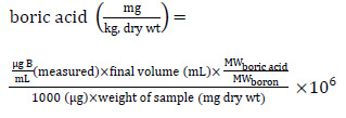
Long description
The concentration of boric acid in soil can be calculated by dividing the molecular weight of boric acid by the molecular weight of boron and then multiplying this result by: the measured micrograms of Boron per milliliter, the final volume (in milliliters), and 1,000,000. This result is then divided by the product of 1000 micrograms and the weight of the sample (dry weight in milligrams).
The analytical limit of detection for boric acid in soil is reportedly 1 mg boric acid/kg soil dry wt in most instances (Stephenson, 2003).
Besides performing acute lethality tests with a reference toxicant, it is recommended that any laboratory performing 21- or 28-day tests with samples of contaminated (field-collected or chemical-spiked) soil also conduct one or more 21- or 28-day test(s) with their culture(s) of F. fimetaria and P. minuta, or F. candida and O. folsomi, respectively, using a reference toxicant. In keeping with the guidance in EC (2004a, 2005a), these tests should either be performed at least twice a year or, where the testing of contaminated soil is carried out at a lesser frequency, in parallel with each definitive soil toxicity test. The procedures and conditions to be applied to these 21- or 28-day toxicity tests should be consistent with those described in Section 4 herein. Any endpoint data (i.e., 21- or 28-day LC50 and/or ICp; see Section 4.8) should be compared with values obtained in the past for the same species, by the same laboratory and for the same reference toxicant. This testing and comparison is useful to provide assurance that the laboratory’s test conditions and procedures when performing a 21- or 28- day test are adequate, and to verify that the long-term response of the springtails to the reference toxicant has not changed appreciably from that of earlier long-term tests with this chemical performed at the testing facility. Boric acid spiked in artificial soil is the recommended reference toxicant for this 21- or 28-day test.Footnote86