
Climate guidelines overview
Stefan Michalski
Disclaimer
The information in this document is based on the current understanding of the issues presented. It does not necessarily apply in all situations, nor do any represented activities ensure complete protection as described. Although reasonable efforts have been made to ensure that the information is accurate and up to date, the publisher, Canadian Conservation Institute (CCI), does not provide any guarantee with respect to this information, nor does it assume any liability for any loss, claim or demand arising directly or indirectly from any use of or reliance upon the information. CCI does not endorse or make any representations about any products, services or materials detailed in this document or on external websites referenced in this document; these products, services or materials are, therefore, used at your own risk.
On this page
- List of abbreviations
- Introduction to guidelines and specifications
- Purpose and limitations of climate guidelines
- There are no standards but many guidelines
- How to find your climate guidelines
- The role of the “Museums, Galleries, Archives, and Libraries” chapter
- Integration with building design, microclimate design and sustainability
- Incorrect climate is one risk among many
- Time-lapse videos of deterioration
- Appendix A: The four parameters of a climate specification
- Appendix B: Sensitivity to fluctuations and the application of proofed fluctuations
- Appendix C: The response times of objects and the multiple benefits of enclosures
- The meaning of response time
- The meaning of enclosures
- Integration of enclosures with the building and its systems
- Relative humidity response times of objects with and without enclosures
- Charts for the response time of wooden objects
- Concerns about temperature fluctuations on microclimate enclosures
- The effect of temperature on response times
- Equations behind the calculations of response time
- Bibliography
List of abbreviations
- ACH
- air changes per hour
- ACD
- air changes per day
- ASHRAE
- American Society of Heating, Refrigerating and Air-Conditioning Engineers
- CCI
- Canadian Conservation Institute
- RH
- relative humidity
- SI
- International System of Units
Introduction to guidelines and specifications
In this resource, the term “guidelines” will mean both qualitative and quantitative advice on climate control methods for large and small museums, whether by mechanical systems, microclimate enclosures or simply by leaving well enough alone. In contrast, a climate specification is a numerical set of performance targets needed by designers (usually of mechanical control systems, but sometimes of exhibit cases, shipping crates, etc.).
Climate specifications for museums have been, and remain, complex and contentious. They can significantly affect a museum’s traditional financial budget as well as its carbon footprint budget, which has become increasingly important. Climate specifications have usually been aimed solely at the designers of mechanical systems, but meeting those targets in the long term will only be feasible and sustainable if the museum integrates the design of the mechanical system with the design of the building and its microclimate enclosures. In many scenarios, it will either be the building alone or the enclosures alone that reliably achieve the specifications. When making decisions about climate control, all three elements must be considered: the building envelope, mechanical systems and microclimate enclosures.
Purpose and limitations of climate guidelines
The climate near an object [that is, the temperature and relative humidity (RH)] sometimes has a big effect on the preservation of that object. Other times, it does not. For some objects, it is the temperature that matters most; for others, it is the RH. Sometimes, the average conditions are most important. At other times, it is the fluctuations. A single object can contain many components, each with conflicting requirements in terms of climate. A collection can contain many different types of objects. Eventually, you must ask how significant these effects are and what loss of value they cause. Determining what climate the collection actually requires is complicated.
A second list of climate requirements comes from the staff and visitors, who want human comfort. And a third list of climate requirements comes from the building, which is very often a part, or even the largest part, of the heritage asset.
A fourth and, until recently, invisible, list of requirements comes from our planet. Any attempt by an institution to maintain a particular climate will consume time, money and, most importantly, energy, all of which are in conflict with the sustainability of our planet and our need to limit climate change.
Climate guidelines for heritage institutions are an attempt to satisfy the requirements associated with all four of these elements: the collection, the people, the building and the planet. Trying to meet all possible requirements is usually hopeless, since few overlap. This then becomes a human argument because different stakeholders champion their own sets of requirements. The only feasible approach is to try to define and then meet the essential climate requirements of all four elements (Michalski 1998).
In a risk management approach, you make such decisions by asking each group what is the worst, rather than the best, that can happen for them. In other words, you find a climate specification that minimizes the total risk. The challenge with this approach is that it cannot be generalized accurately. The risks to the collection, those to the building, those to the occupants and those to the planet all depend on value judgments. It is very much a case of think and value globally, but act and value locally.
There are no standards but many guidelines
Numerous organizations, both standards bodies and professional associations, have published climate guidelines. Consult Michalski (2016) for a recent review of their differences and the history of their origins.
Climate specifications and climate guidelines for museums, galleries and archives are sometimes mistakenly called “climate standards.” Unlike building codes driven by life safety concerns, there are no legally binding standards for climate control in heritage institutions. There are, however, legal contracts between lending and borrowing institutions that usually include climate specifications that must be met. For certain government programs, such as the Designation of Institutions and Public Authorities Program or the Canada Travelling Exhibitions Indemnification Program, designation depends on meeting a particular climate specification.
How to find your climate guidelines
To begin the selection process for a climate guideline, start with ClimaSpec. This search tool provides specific information about the role of temperature and RH for each type of object. It provides guidelines for climate control as well as possible climate specifications (in terms of the nomenclature used in the ASHRAE Handbook: Heating, Ventilating, and Air-Conditioning Applications). ClimaSpec also has a mould calculator and a lifetime calculator (consult the Explanation of the mould and lifetime calculators page for background details). As a supplement to its climate advice, ClimaSpec provides information on the role of pollutants and their control, since filtration is always part of a climate control system.
After using ClimaSpec, you may find that your collection contains several different categories of objects in terms of sensitivity to fluctuations. You may also wonder how a designation under the Designation of Institutions and Public Authorities Program or your participation in Canada’s Indemnification Program will influence your climate control decisions. The Climate Control Decision Tool asks a sequence of questions that directs you to specific pieces of advice related to a climate guideline.
The role of the “Museums, Galleries, Archives, and Libraries” chapter
Since the first edition of the ASHRAE Handbook in 1999, the Canadian Conservation Institute (CCI) has adopted the “Museums, Galleries, Archives, and Libraries” chapter as its primary source for climate control specifications. The ASHRAE Handbook is the primary reference manual for mechanical engineers in Canada, the US and many other countries. Committees of technical experts write its chapters via discussion and consensus, and then the American Society of Heating, Refrigerating and Air-Conditioning Engineers (ASHRAE) membership reviews their work. CCI staff members were part of the technical committee that created the original 1999 chapter. It has been the aim of both CCI and the chapter committee to write guidelines that could be trusted by engineers as well as the heritage community. One of the committee’s most significant innovations are the levels of control (now called “types of control”) labelled AA, A, B, C and D, which have since been widely adopted in the heritage community.
In the 20 years between the 1999 and 2019 editions, chapter content on temperature and RH had remained unchanged, but sustainability — environmental, economic and financial — has forced climate control thinking to evolve further, not only in our field but also throughout the heritage sector. This evolution is evident throughout the 2019 edition. A risk management perspective has become essential. What are our preservation goals, and what are the costs and benefits of each type of control?
For the 2019 edition, the chapter committee revised the chapter completely, starting with a risk management introduction, followed by an emphasis on selecting an annual average that is as energy efficient (sustainable) as possible. This replaced a universal and often wasteful guideline of 50% RH and 20°C. The categories AA, A, B, C and D are still in place, albeit slightly modified. Sub-types of low-temperature storage (cool, cold and frozen) were revised to be consistent with recent guidelines from the International Organization for Standardization and the Image Permanence Institute (IPI). Specifications for temporary exhibit space and unpacking space for loaned objects were given a separate category. (The sections on pollution and on system design were also completely revised.) As in 1999, CCI staff members were part of the committee in 2019, and CCI fully supports the 2023 edition that was available at the time of writing.
While CCI recommends that anyone engaged in a project involving climate control decisions should obtain a copy of the most recent version of the ASHRAE chapter, this resource provides explanations of all key issues. The ASHRAE types of control page summarizes the ASHRAE climate specifications, and ClimaSpec provides specific recommendations for individual groups of objects.
Integration with building design, microclimate design and sustainability
As emphasized in the ASHRAE Handbook, you cannot begin to select a design target for the mechanical systems without first considering the local climate, the building envelope and the use of microclimate enclosures. It is outside the scope of this resource to examine these issues in detail, but they can be summarized as follows.
For any collection, whether planning the design of a new building or working within an old building, consider the following:
- Use ClimaSpec to find out what climate your collection actually requires and what damage is possible if you do not meet these requirements.
- From a risk management perspective, establish what this possible damage means to your collection in terms of loss of value. Determine what is acceptable and what is not. This varies with your institution’s mandate and any legal obligations. What balance do you wish to make between preservation, accessibility and your budget? Consult “Step 1: Establish the context” in The ABC Method: A risk management approach to the preservation of cultural heritage.
If you are planning the design of a new building, consider the following:
- Share an understanding of the ASHRAE Handbook chapter “Museums, Galleries, Archives, and Libraries” and this online resource with staff and consultants.
- Recognize sustainability as a fundamental design issue and a win-win perspective rather than an addendum to be lost during inevitable budget trimming.
- Recognize the role of microclimate enclosures, specifically in reducing response times to fluctuations and exposure to pollutants (consult Appendix C: The response times of objects and the multiple benefits of enclosures). Integrate these benefits into the design of the building and its mechanical systems.
If you are working with an existing building, consider the following:
- Apply the latest energy management tools to the building and its systems to obtain not only energy savings but also improved performance and reliability. For basic energy tracking and benchmarking, consider using Portfolio Manager from Energy Star. RETScreen is a more advanced tool offered by Natural Resources Canada, with additional features for feasibility assessments and performance analysis of facilities. RETScreen training courses are offered by the Canadian Institute for Energy Training (CIET), and free resources are available on the YouTube RETScreen eLearning channel.
- Recognize that microclimate enclosures play an even more important practical role in climate control when the whole space cannot be brought to desired conditions, specifically in reducing response times to fluctuations and exposure to pollutants (consult Appendix C: The response times of objects and the multiple benefits of enclosures). Integrate these benefits into the design of the building and its mechanical systems.
- Recognize that the “proofed fluctuation” concept is especially powerful when making decisions about sustainable climate control for permanent collections. If the collections have been in the same location for many years, and the same pattern of climate fluctuations occurs each year, then the worst cracks and deformations that can be caused by that pattern of fluctuations have already occurred. This concept is described further in Appendix B: Sensitivity to fluctuations and the application of proofed fluctuations, as well as in Agent of deterioration: incorrect relative humidity.
Incorrect climate is one risk among many
CCI made comprehensive risk assessments of five heritage institutions in order to uncover any patterns of common risks. In the two historic house museums and the art gallery, the top three risks to the collections (and to the building if it is part of the heritage asset) did not include incorrect climate. Consistently, the top risks were fire, water damage and physical forces (Karsten et al. 2012). In the provincial archives and the science and technology museum, however, incorrect temperature was a significant risk due to the rapid deterioration of some photographic materials and acidic paper housed at room temperature.
Smaller museums in historic buildings that have operated for many years without special climate control sometimes decide that they need to acquire museum-grade climate control. For a permanent collection that has been in place for decades and has not received conservation treatment, the worst cracks and deformations that can be caused by temperature and RH fluctuations have already happened. If, however, it is known that the climate in the museum building has worsened recently, then analyze what has changed, why and how you might return to the previously proofed and non-threatening pattern.
Some forms of incorrect climate do continue to damage collections. For example, damp will cause mould over a certain period of time, which you can estimate by using the Mould Calculator in ClimaSpec. Causes and solutions for damp are outlined in Figure 5 of Agent of deterioration: incorrect relative humidity.
Pollutants can be considered a form of incorrect climate, and filtration is usually part of a climate control system. As with damp, pollutants cause damage that accumulates. Causes and solutions for pollutants are described in Agent of deterioration: pollutants.
Time-lapse videos of deterioration
Most of the deterioration processes due to incorrect temperature or incorrect RH are slow. It takes days, if not weeks, for them to emerge. To demonstrate some of these processes, CCI has created time-lapse videos that illustrate some of the deterioration phenomena.
Appendix A: The four parameters of a climate specification
Parameter 1: Long-term outer limits or danger boundaries
Long-term outer limits are danger boundaries in RH and temperature beyond which mixed collections may be at increasing risk of damage. When the annual average (baseline) selected is far from the traditional middle values of 50% RH and 20°C and this baseline is then combined with suggested seasonal adjustments, the resulting range of temperatures and RH could exceed these danger boundaries for a mixed collection. This is illustrated in Figure 15 in the “Museums, Galleries, Archives, and Libraries” chapter of the ASHRAE Handbook. ASHRAE control types C and D are defined solely in terms of their long-term outer limits.
The particular deterioration phenomena that determine the setting of danger boundaries are discussed in the following sections.
Mould
While it is not possible to avoid common species of bacteria and mould, you can prevent the damp conditions that allow their growth. Bacteria require RH bordering on wet conditions (over 99% RH), but mould can grow at an RH as low as 65%. Detailed data about the relationship between RH and mould growth is shown graphically on the Explanation of the mould and lifetime calculators page. ClimaSpec uses equations derived from these graphs to calculate the days to mould growth at different relative humidities.
Lifetime of chemically decaying organic materials
As discussed further in the section Parameter 2: Annual averages or baseline, some objects decay rapidly at human comfort temperatures, some decay moderately quickly and others decay very slowly. These rates of decay all double (approximately) for every rise of 5°C. The ASHRAE Handbook suggests upper limits for each type of control as a warning that everything organic in mixed collections will last less than half, or less than one quarter, of its lifetime when temperatures exceed those limits. Where available for specific materials, ClimaSpec provides more specific advice about outer limits than what is suggested in the ASHRAE chapter.
Chemical decay of metals and minerals
Moisture causes and accelerates the corrosion of metals and the disintegration of many minerals. The dependence on humidity usually jumps suddenly at a critical RH due to hydration or to deliquescence of a salt, so the critical RH values become danger boundaries. Where available, ClimaSpec provides these critical RH values to establish specific danger boundaries for metals and minerals.
Physical transformations
Some materials will soften, or even melt, at sufficiently high temperatures. Others will become brittle and fragile at sufficiently low temperatures. Consult Agent of deterioration: incorrect temperature for an overview and ClimaSpec for specific objects. For some heritage objects, these damaging temperatures are within the range of potential natural exposures outdoors, certainly, and often indoors.
Parameter 2: Annual averages or baseline
Temperature and RH values that satisfy human comfort are not necessarily satisfactory for collection preservation. Cooler and dryer conditions preserve all materials longer but are uncomfortable for occupants. Maintaining cool or dry conditions in summer is also energy intensive. A climate control decision considers the wide range of lifetimes in a typical collection and balances them with human comfort and sustainability.
Lifetime of chemically decaying organic materials
The annual baseline recommendation presumes that an institution wants its collections to remain in a good state of preservation for at least a century, if not longer. Natural materials such as wood, cotton and linen last thousands of years at normal room conditions, but only if they have not been acidified during manufacture or during exposure to pollution. On the other hand, acidic papers become brown and brittle within decades (consult Caring for Paper Objects); acidified leather book bindings disintegrate; films, audiotapes and videotapes become sticky, shrivelled and unplayable (consult Caring for Audio, Video and Data Recording Media); and celluloid plastics and polyurethane foam become yellow and disintegrate (consult Caring for Plastics and Rubbers).
Acid hydrolysis is the major mechanism behind the decay of all these particularly unstable materials, and this process needs moisture. The rate of decay of these materials decreases by a factor of about two for each 5°C drop in temperature and by another factor of about two for each halving of RH. You can make detailed estimates of the remaining lifetime for various scenarios of temperature and RH using the Lifetime Calculator in ClimaSpec. All the technical background for such calculations is contained on the Explanation of the mould and lifetime calculators page.
Human comfort
This resource focuses on the preservation of collections and the sustainability of the design solution in a museum environment, not on human comfort. Of course, a final specification for a project will balance human comfort with the risks and benefits to the collection (and with sustainability). Very different compromises can be made in display areas and storage areas in terms of temperature and RH. Enclosure solutions allow RH for particular objects to be controlled distinctly from the room.
Local climate and building envelope capability
Local climate and the characteristics of the building envelope determine the feasibility and sustainability of any climate control target. These issues were more strongly emphasized in the 2019 and 2023 editions of the ASHRAE chapter than in previous editions. The annual baseline selected for temperature and RH, in combination with seasonal adjustments, will determine the size of climate control systems and their energy consumption.
Parameter 3: Seasonal adjustments from the annual average or baseline
Seasonal adjustments are intentional changes in the temperature and RH settings designed to reduce energy consumption in winter and summer. Seasonal adjustments have been common in smaller museums and galleries but were considered less than ideal and inappropriate for larger institutions. This attitude has shifted in favour of sustainability. The 2019 and 2023 editions of the ASHRAE chapter emphasize that sustainability considerations should play a much larger role in decisions about seasonal adjustments, regardless of the scale of the institution.
Parameter 4: Short-term fluctuations plus space gradients
Short-term fluctuations, or simply short fluctuations, may be caused by the mechanical system cycling on and off many times per day, by the day-night cycle or by the effects of the weather outside. Short fluctuations can be unintentional, as in the typical sawtooth pattern of a simple system switching on and off, or it can be intentional, as in a complex system that is designed with a deadband between opposing processes, such as heating versus cooling and humidification versus dehumidification. The word “short” was not defined in the 1999 to 2015 editions of the ASHRAE chapter, and users often asked for clarification. In the 2019 and 2023 editions, the following note was added: “Short-term fluctuation means any fluctuation shorter than the times specified […] for rate of seasonal adjustment (i.e., 30 days for relative humidity fluctuations, 7 days for temperature fluctuations).” (ASHRAE 2023)
Space gradients refer to the change in RH and temperature that occurs between a hot or cold wall or floor and the room average. It also refers to the change between the air supply vents and the return air conditions. Of course, in real systems such gradients are unavoidable and often large. This specification is not aimed at every location in the room; it is only aimed at the locations where collections are held. It is not intended to lead to designs with unusually high air exchange rates and high energy consumption. Rather, it is intended to encourage the adoption of as many passive design features that reduce gradients as possible (for example, high insulation of the envelope, good distribution of air movement, as well as adequate separation of collection fittings and collection objects from obvious sources of such gradients). Such advice applies as much to simple systems in historic buildings as it does to purpose-built facilities with sophisticated systems. Consult Figures 5 and 6 in Agent of deterioration: incorrect relative humidity.
System failure is a bigger risk than routine fluctuations
From a risk management perspective, the most important fluctuations are the occasional extreme fluctuations caused by system failure, such as a very low RH due to humidification failure during a cold winter or high humidity in summer due to faulty air conditioning. A once-in-30-years extreme event in RH is much more damaging to an unpackaged collection than a modest increase in the size of short fluctuations throughout those 30 years. Long-term reliability remains a secondary concern in many mechanical system designs, and an example where enclosures, such as moistureproof packaging of objects and sealed cabinets, play an essential role in collection risk management. Consult Appendix C: The response times of objects and the multiple benefits of enclosures.
Sensitivity to fluctuations and the proofed fluctuation
The sensitivity of objects to fluctuations in RH and temperature has been the single most contentious issue in setting climate control specifications, and it often becomes an obstacle to more sustainable climate control decisions. The issue of object sensitivity and the role of history in establishing a proofed fluctuation are discussed in more detail in Appendix B: Sensitivity to fluctuations and the application of proofed fluctuations.
Appendix B: Sensitivity to fluctuations and the application of proofed fluctuations
Four levels of initial sensitivity to fluctuations
In previous publications, we have used the terms “vulnerability” and “sensitivity” interchangeably. Here, sensitivity will refer to the physical response of an object to an agent of deterioration, such as fracture due to RH fluctuations, whereas vulnerability will refer to the consequent loss of value, which depends on many additional factors.
By “initial sensitivity,” CCI means the sensitivity level of an object to temperature and RH fluctuations on the day it was made (assuming it has reached equilibrium with its local RH), before any fluctuations have taken place. After the object experiences some fluctuations, it is said to be “proofed” to that size of fluctuation, and it is no longer sensitive to less extreme fluctuations (Michalski 1993, 2007). If fractures in an object are adhered, however, then the object returns to a new initial, unproofed state.
Different objects have different sensitivity levels to fluctuations in temperature and RH. The level of initial sensitivity (before any exposure to fluctuations) is determined by the following four factors:
- The amount that the reactive components expand and contract for a given size of fluctuation (the expansion coefficient).
- The elasticity of affected components, which depends on the age of the material as well as the temperature and RH prior to the fluctuation.
- The geometry of the assembled components. Are reactive components restrained, or, worse, are weak, brittle components attached to strong, reactive components?
- Unevenness in the thickness of stressed components or their attachment to restraining components, which causes localized stress concentration.
For practical purposes, objects with materials that respond to RH can be divided into four categories, each twice as sensitive to fluctuations as the previous, as shown in Table 1.
| Low sensitivity (half or less of medium sensitivity) | Medium sensitivity | High sensitivity (double the sensitivity of medium) | Very high sensitivity (double the sensitivity of high) | |
|---|---|---|---|---|
| Type of assembly and component flaws | Components are free to move relative to each other | Uniform restraint of components (distributed attachment) and no notches | Uneven restraint of a component or uniform restraint plus notches | Uneven restraint plus localized movement, such as a paint layer or veneer across a moving wood joint |
| Approximate stress concentration | ×1/2 or less | ×1 | ×2 | ×4 |
| Damage at ±40% RH | Between no damage and small damage | Small to severe damage (benchmark 1) | Severe damage (benchmark 2) | Very severe damage |
| Damage at ±20% RH | Between no damage and tiny damage | Between no damage and small damage | Small to severe damage | Severe damage |
| Damage at ±10% RH | No damage | Between no damage and tiny damage | Between no damage and small damage | Small to severe damage |
| Damage at ±5% RH | No damage | No damage | Between no damage and tiny damage | Between no damage and small damage |
The lower four rows in Table 1 map the degree of damage expected for various combinations of RH fluctuation (rows) and object sensitivity (columns). The degree of damage is determined by extrapolating from the cell that contains benchmark 1. Benchmark 1 is based on the common observation as well as available experimental evidence that evenly restrained responsive materials will probably not fracture in one cycle until the humidity goes from a middle value near 50% RH (common in summer in Canada) down to a very low value of about 10% RH (common in heated buildings in winter). Examples of responsive materials that are evenly constrained include wood panels held evenly at their edges, oil paintings on canvas with uniform layers of paint held evenly by a strainer or skins stretched uniformly in a kayak or umiak.
Furthermore, we can observe that when cracks or tears do occur (severe damage), they are located at flaws or notches, which corresponds to the cell that contains benchmark 2. The remainder of the table is extrapolated from these benchmarks.
Note that each diagonal row of cells (from top left to bottom right) predicts the same degree of damage. This is because these diagonals link cells of equal stress: as you move one step down in the table, the fluctuation size is halved; as you move one step to the right, stress concentration doubles. For the same reasons, each diagonal has double the stress of its neighbour to the left.
Table 1 does ignore four known corrections to the stresses created by fluctuations, but these corrections would not change the four broad categories of sensitivity. Besides, all four corrections tend toward making Table 1 conservative in its advice. The four corrections are the following:
- Stress in wood, leather, paper, plastics, coatings, etc., relaxes over time, so very slow fluctuations cause less stress. Consult Michalski (2007) for further discussion.
- Objects take time to respond to fluctuations. If the fluctuation is shorter than the object’s response time, stress is less than predicted. This is discussed further in Appendix C: The response times of objects and the multiple benefits of enclosures.
- The phenomenon of hysteresis during RH fluctuations means that a fluctuation of ±20% RH causes less than half the dimensional change of ±40% RH, a fluctuation of ±10% RH causes less than half the dimensional change of ±20% RH and a fluctuation of ±5% RH causes less than half that of ±10% RH. Since the table is built from the historic evidence of fracture at ±40% RH, then hysteresis makes the extrapolations of stress to smaller fluctuations progressively less than estimated in Table 1.
- The humidity expansion coefficient varies with RH. When plotted as a function of RH, it follows an S-shaped curve. Below 25% RH and above 75% RH, the coefficient progressively increases. The result is that a fluctuation of ±40% RH (top row of Table 1) will cause more than just double that of ±20% RH. (This correction to the relationship between ±40% RH and ±20% RH is in addition to the hysteresis correction which applies to all steps between ±40% RH and ±5% RH.) In summary, the simplified extrapolation to rows with smaller fluctuations than ±40% RH yields cautious estimates.
Expressions of damage in the cells of Table 1 for high and very high sensitivity appear at first glance to suggest that a great deal of damage across collections will occur during relatively small fluctuations. These categories, however, never apply to a whole object or even most of the object in the sense of the whole object disintegrating. Common sense and experience tell us that the world did not fall apart before modern climate control. High and very high sensitivity applies to specific locations within objects and usually to badly designed objects from the perspective of durability. For example, it applies to the paint that crosses a weakened joint in a lacquered wooden chair or a panel painting, the paper near pins holding a large sheet to a rigid frame and the skin of an umiak where it is attached to the frame with too few cords that are also too narrow. Since in historic items, those locations fractured long ago, it can only refer now to the repairs and infills bridging those same locations.
The ASHRAE chapter contains an extensive table that expands on the generic content of Table 1. ClimaSpec uses that table, and other sources, to provide quick access to specific sensitivity assessments of each collection or object that you wish to understand.
Initial sensitivity to fluctuations is not a precise science
Specific numbers used to specify fluctuations in this resource, such as ±10%, ±20%, ±5°C and ±10°C, should not be taken to mean that the science is precise to within 1% RH or 1°C and that risk suddenly changes at precisely these values. These are round numbers based on the best available estimates of risk. Numbers such as ±8% RH or 6°C have not been employed because they might imply a precision that does not exist at present. [Unfortunately, conversion of these round numbers, that originated in SI (metric) units, into US customary units, as needed for the ASHRAE inch-pound (I-P) edition, creates numbers that are not round, but they must be left as is for consistency.] Even if one day the science does become very precise, it will only provide a precise probability of damage at each fluctuation and not a guarantee that fracture occurs precisely at that fluctuation.
A loan contract is a precise obligation
Refining recommendations for the long-term preservation of your own collections does not remove contractual obligations entered into for loans or for programs such as the Designation of Institutions and Public Authorities Program or the Canada Travelling Exhibitions Indemnification Program. A precise specification in a design contract or a loan contract is a precise statement of obligations, even if it borrows round numbers from an imprecise science. Unfortunately, it is not easy to measure actual RH conditions with sufficient precision to know if the contract has been met. Measuring RH to better than ±5% RH requires costly instrumentation. As noted elsewhere, there is only one way to guarantee climate safety with regards to precious objects: a reliable microclimate enclosure.
Collection history and proofed fluctuations
Cracks in objects, that is delaminations as well as visible cracks, cannot form again in the same location, unless the old fracture has been reattached or adhered. When exposed to the same fluctuation that caused the crack, the crack simply opens and closes (Michalski 1993, 2007). Studies of cracks in wood furniture located in buildings with wide but consistent fluctuations, and for which historic photographs are available, have shown that the cracks were indeed all old and had not visibly progressed (Ekelund et al. 2018). Recent analysis of the mechanics of paint layers suggests that craquelure reaches saturation, beyond which new cracks will not develop (Wu et al. 2014; Bratasz and Vaziri Sereshk 2018). Such limits on accumulation of damage despite reoccurrence of the hazard is very different from other deterioration processes that continue to accumulate until the material disintegrates, such as repetitive events of mould, continual chemical deterioration, light fading and pollution damage. If the largest fluctuation experienced by an object in the past was a 30% RH drop from an annual average of 50% RH (a drop to 20% RH), then all the mechanical damage likely to occur from a single fluctuation of that size has already occurred. Therefore, a future drop in RH that is slightly smaller than this previous drop of RH cannot cause a new crack.
Proofed fluctuation, as established by previous climate history, is extremely important in establishing realistic and sustainable targets that cause low risk to collections. The Climate Control Decision Tool asks about climate history in some situations in order to establish collection sensitivity. Similarly, ClimaSpec identifies different sensitivities and recommendations depending on the climate history of the object or collection.
Fatigue fracture
Many thousands of additional fluctuations similar to the one that is considered the object’s proofed fluctuation can lead to further crack growth through a process called “fatigue.” This is a subtle correction to the application of proofed fluctuation, and it has been incorporated into advice provided by ClimaSpec.
Figure 1 and Tables 2 and 3 come from a review (Michalski 2014) of the best available fatigue studies for materials essential to heritage collections: wood, paints and gesso. Plots such as those in Figure 1 are called S-N curves (stress versus number of cycles) or Wöhler curves. The S-shaped curve usually drawn through S-N curves has been simplified to three straight lines:
- the initial plateau that falls from 1 to about 0.9 at 30 cycles,
- the transition region from 30 to over 300,000 cycles and
- the final plateau, known as the “endurance limit,” that begins at about 1,000,000 cycles.
At the endurance limit, fatigue damage ceases. Although of interest to vibration studies, exposure to 1,000,000 cycles (that is, 1,000,000 fluctuations) is far beyond what is relevant for daily fluctuations (2,700 years), let alone seasonal fluctuations.
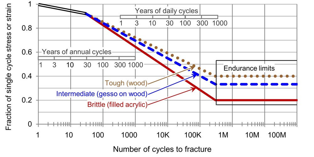
© Government of Canada, Canadian Conservation Institute. 132715-0029
Figure 1. Fatigue graph (S-N curves) for materials that range from tough to brittle (Michalski 2014).
Description for Figure 1
Figure 1 contains a single graph with three plots. The horizontal axis is a logarithmic scale of the number of cycles to cause fracture, and the vertical axis is the stress or strain that causes that fracture, expressed as a portion of the stress or strain that causes fracture in one cycle. The three plots all begin on the left at x = 1 and y = 1. They drop towards the lower right at x = 1 million cycles and y values between 0.2 and 0.4.
| Type of materials | 1 year | 3 years | 10 years | 30 years | 100 years | 300 years | 1000 years |
|---|---|---|---|---|---|---|---|
| Tough materials, such as wood | 1 | 0.98 | 0.95 | 0.92 | 0.84 | 0.78 | 0.71 |
| Intermediate materials, such as gesso on wood | 1 | 0.98 | 0.95 | 0.92 | 0.83 | 0.75 | 0.70 |
| Brittle materials, such as filled acrylic | 1 | 0.98 | 0.95 | 0.92 | 0.82 | 0.72 | 0.46 |
| Type of materials | 1 year | 3 years | 10 years | 30 years | 100 years | 300 years | 1000 years |
|---|---|---|---|---|---|---|---|
| Tough materials, such as wood | 0.78 | 0.71 | 0.65 | 0.59 | 0.51 | 0.45 | 0.40 |
| Intermediate materials, such as gesso on wood | 0.76 | 0.69 | 0.62 | 0.54 | 0.48 | 0.39 | 0.32 |
| Brittle materials, such as filled acrylic | 0.72 | 0.63 | 0.45 | 0.35 | 0.29 | 0.28 | 0.20 |
The lines in Figure 1, or the rows in Tables 2 and 3, can be thought of as equivalent combinations of fluctuation size and fluctuation number. For example, following the last row of Table 3 for brittle materials such as filled acrylic, a single annual fluctuation of size ±X% RH is equivalent to 30 years of annual fluctuations of size 0.92 × ±X% RH or to 100 years of annual fluctuations at 0.82 × X% RH, and so on.
In practice, even daily or weekly fluctuations are unlikely to be precisely the same size, so fatigue, even from daily or weekly fluctuations, is determined simply by the biggest fluctuation of the year (the winter and summer peaks). It is the scale of annual fluctuation shown in the lower left corner of Figure 1, and provided in Table 2, that concerns us.
To obtain an estimate of future risk, based on a history of many fluctuations, rather than just one historic fluctuation, you use the ratio of the future and historic factors. As an example, if you know that for the last 30 years there has been a consistent annual fluctuation of size ±X% RH, and you want to know what is a safe fluctuation for the next 100 years for a brittle material, then find in Table 2 the factor for 30 fluctuations (0.92) and the factor for 100 fluctuations (0.82). Now calculate the ratio of those two factors (the factor for 100 years ÷ the factor for 30 years), which is 0.82 ÷ 0.92 = 0.89. If you know that in the last 30 years, RH had an annual average near 50% but fluctuated by ±30% (so down to 20% RH each winter), then keeping future fluctuations at or below 0.89 of ±30% RH (that is, ±27% RH) will provide safety for the next 100 years. In other words, do not let winter RH drop by more than 27% from the average of 50% RH (do not go below 23% RH).
Note that this is not a huge difference from the 20% RH of the last 30 years. Very slight reductions in fluctuation from the worst historic fluctuations have huge benefits.
You can read these fractions directly from Figure 1 or Tables 2 and 3, or you can use the following equation for the middle portion of the plot for brittle material, which is good for the range of 30 cycles to 300,000 cycles.
Equation 1: ±Xf% RH = ±Xh% RH * {[0.18*log10(nh) + 1.19] / [0.18*log10(nf) + 1.19]}
Where
±Xf% RH = maximum future fluctuation that must not be exceeded
±Xh% RH = size of known historic fluctuations
nh = number of known historic cycles (30 and above)
nf = number of future cycles to consider (maximum 300,000)
In summary, fatigue refines the proofed fluctuation concept as follows: for every n years of known historic pattern of fluctuations, you can project that staying within this proofed pattern for the next n years will cause very low risk of new fractures. Furthermore, if you make very modest reductions in future fluctuations compared to the proofed pattern, then you can project many times further than n years.
Do not hide how bad your climate control might have been in the past. This history of proofed fluctuations is the best estimate of the sensitivity of any collection and the best guide when choosing sustainable options for climate control.
Damp can reduce a proofed fluctuation
At a very high RH (well over 75%), wood can be crushed if it is prevented from expanding (for example, tenons held tightly within a mortise). On return to moderate RH, the wood remains crushed. At a very high RH, the animal glue holding these joints and veneers in place changes from strong and inflexible to weak and pliable and to almost a jelly near 100% RH. As a result, the components of joints and veneers in furniture that were exposed to damp will re-adhere in slightly changed positions when they return to moderate RH. In extreme cases, veneers detach and buckle when damp and remain buckled when RH returns to moderate values. A proofed fluctuation that was established in the range of 0% to 75% RH might be reduced after a period of damp. CCI has observed this effect in veneered wood joints using acoustic emission (Hagan 2021). We can expect that other objects based on animal glue or size, such as paintings on canvas, may suffer from the same effect.
In practical terms, periods of damp not only cause severe mechanical damage in and of themselves, but they can reduce a proofed fluctuation that was established for fluctuations that occurred below 75% RH. The extent of such reduction remains uncertain.
Appendix C: The response times of objects and the multiple benefits of enclosures
This Appendix provides technical background to the response time estimates of ClimaSpec. It also explains why integrating microclimate enclosures into building design and mechanical systems is essential for a sustainable, risk-based approach to collection use and collection care.
The meaning of response time
When an object at equilibrium with its surrounding temperature and RH is exposed to a change in temperature or RH, it takes time to fully respond (to reach a new equilibrium with its new environment). The general form of the response is a curve, as shown by the lower graph in Figure 2.
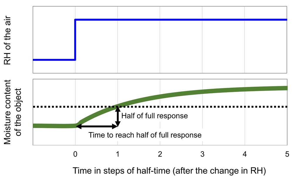
© Government of Canada, Canadian Conservation Institute. 132715-0031
Figure 2. Moisture content change in an object over time, in response to a sudden change in RH of the surrounding air.
Description for Figure 2
Figure 2 contains two graphs. The horizontal axis is time, shown in steps of half-time. The top graph is for RH, showing a single sharp step from an initial RH to a steady final RH. The bottom graph is for the moisture content of the object, and it shows a smooth gradual climb to a final plateau of full response to the RH change. A horizontal dashed line marks the midway level of this moisture content curve.
The response time (also called the half-time) is specified as the time it takes to reach one half of the eventual maximum response. There are several advantages to specifying half-time rather than a full response. Half-time is unambiguous; whereas the phrase “full response” depends on what fraction of the response is a full response. Is it 90%, or 99% or 99.9% of the eventual change? Half-time also has the advantage of providing a conservative estimate of the time period within which you should act to reduce risks due to a fluctuation.
The meaning of enclosures
For climate control purposes, an enclosure is any bag, box, case, cabinet, crate, etc., that reduces contact between an object’s surface and the humidity and pollutants in the room. In practice, this means not only that the enclosure material has low permeability to moisture or pollutants, but also that the enclosure is relatively airtight, since in most situations, the primary path for moisture and pollutants are small openings in the enclosure. (Details are given in the following sections.) Although you can also think of a new or historical coating on an object as a form of enclosure, for preventive conservation advice, CCI means only enclosures that are easily removed when necessary.
Integration of enclosures with the building and its systems
From a risk management perspective, the risks to collections from various kinds of RH fluctuations can be divided into two very different types (Michalski 2016):
- Frequent events: The routine fluctuations of hours, days and seasons that, over time, determine the proofed fluctuations of the collection. These may be caused by natural cycles of the outdoor climate or by routine fluctuations of the mechanical system.
- Rare events: These are extreme changes in temperature or RH that occur decades or even centuries apart. Very few rare events that have been recorded are natural, such as the exceptionally cold winter of 1928 in London that caused an extreme drop in RH in the National Gallery. Afterwards, staff observed unusual and significant damage to panel paintings, and this observation led to an official research inquiry (Michalski 2016). More commonly, however, these rare events are failures of mechanical systems at the end of their life (typically 30 years), which can create very high or very low RH. (Cold-storage crashes that cause RH to reach 100% become tragedies only when the stored objects are not packaged.) Occasionally, these system events occur at the beginning of a new mechanical system’s life, hence the need for debugging new systems before exposing unpackaged collections. Sometimes these events are the result of a collection’s move into improved RH conditions, after decades of stable storage at a very different annual average of RH.
From a risk management perspective of many decades of preservation, a rare event, or even just a 10% chance of a rare event, is the dominant risk due to climate fluctuations. The only fail-safe against such risks is enclosures. Enclosures are increasingly part of basic preservation strategies and not only for institutions such as historic house museums without climate control (consult Agent of deterioration: incorrect relative humidity – Vignette 2. Simple display boxes that reduce incorrect RH), but also for major museums with precious objects that want to reduce long-term risks (consult Figures 10a and 10b in Basic requirements of preventive conservation).
You might then ask: what purpose do climate control systems serve beyond those needed for human comfort if all objects are in enclosures? Aside from the fact that museums large and small will use the risk-reduction ability of enclosures for targeted objects (objects of exceptional value, exceptional sensitivity and exceptional risk of vandalism), the practical reality is that simple enclosures cannot mitigate temperature changes for more than a few hours and most cannot mitigate seasonal shifts in RH. What even simple enclosures can do is mitigate rare crashes that might last several days or even weeks before repairs are made and rare weather events that overwhelm the system. They also greatly reduce access by external pollutants. (Consult Technical Bulletin 32 Products Used in Preventive Conservation for materials that are not themselves a source of pollutants.) Whereas you might have reasons to avoid enclosures in a display, simple packaging for objects in storage is the only means to rationally obtain long-term risk management (consult Technical Bulletin 32).
In summary, long-term preservation that is also sustainable is dependent on the integration of the strengths of mechanical systems (making the average temperature and RH different from outdoors) and enclosures (smoothing out RH fluctuations, blocking pollutant exposure) with the strengths and limitations of the building. This recognizes that the local climate is not just a design condition but probably a determinant of the proofed fluctuations of local collections.
Relative humidity response times of objects with and without enclosures
Some of the content of the following two sections appeared first in the 1999 edition or the 2019 and 2023 editions of the ASHRAE Handbook chapter “Museums, Galleries, Archives, and Libraries,” prepared by the author while a member of CCI staff but also as a member of the committee responsible for that chapter. The content has been abridged and updated here.
Table 4 provides RH response times for objects and enclosed objects. Where available, direct measurements have been cited. Other estimates are based on calculations, which are explained in the section Equations behind the calculations of response times.
The range of response times may seem extraordinary, but it is the result of two phenomena:
- Response varies as the square of a material’s thickness. A piece of wood that is 50 times thicker will take 2500 times longer to respond. (For example, a 5 cm thick plank in a dugout canoe versus a 1 mm thick piece of wood in a guitar body or violin will take 50 × 50 times longer to respond.)
- The enclosure effect. Compared with open air, a reasonably airtight enclosure can reduce the rate of access of both moisture and pollutants by a factor of 10 to 100 or more. Objects that respond to RH in a few hours in open air, such as watercolours, or tarnish in a few weeks, such as uncoated silver, will take months, if not years, to respond or tarnish in a well-sealed enclosure of impermeable materials. Two examples include a sealed frame with glass and a backing board for watercolours and an airtight display case for silver.
| Time range | Objects | Enclosed objects | Design implications |
|---|---|---|---|
| Greater than 108 seconds (a year or more) |
|
|
|
| Approximately 107 seconds (weeks to months) |
|
|
|
| Approximately 106 seconds (days to a week) |
|
|
|
| Approximately 105 seconds (a day) |
|
|
|
| Approximately 104 seconds (hours) |
|
|
|
| Less than 103 seconds (a few minutes or less) |
|
|
|
Table 4 notes
- Table 4 note 1
-
These objects are only partially enclosed.
- Table 4 note 2
-
Some of these objects have a tradition of enclosures, such as works on paper. Others, such as textiles and costumes, do not.
Technical notes for Table 4: Calculations for objects shaped as flat plates assume exposure on both sides unless noted otherwise (consult the section Equations behind the calculations of response time). Adelstein et al. (1997) and Bigourdan (2012) reported 90% response times. These are converted for Table 4 to half-times by the factor of 0.4, assuming an approximately exponential decay curve such as in Figure 2, where 90% response occurs at 2.4 half-times, so half-time is 1 ÷ 2.4 = 0.42 of the time for 90% of response. Derluyn et al. (2007) measured a 50 mm square experimental book, closed on all sides except the fore-edge. Their times have been adjusted to a more realistic 100 mm depth, so increased by four times (times vary as the square of thickness). Estimates from Michalski (2005) are based on material data plus enclosure leakage equations. Estimates for wooden objects and furniture are based on Figures 3 and 4.
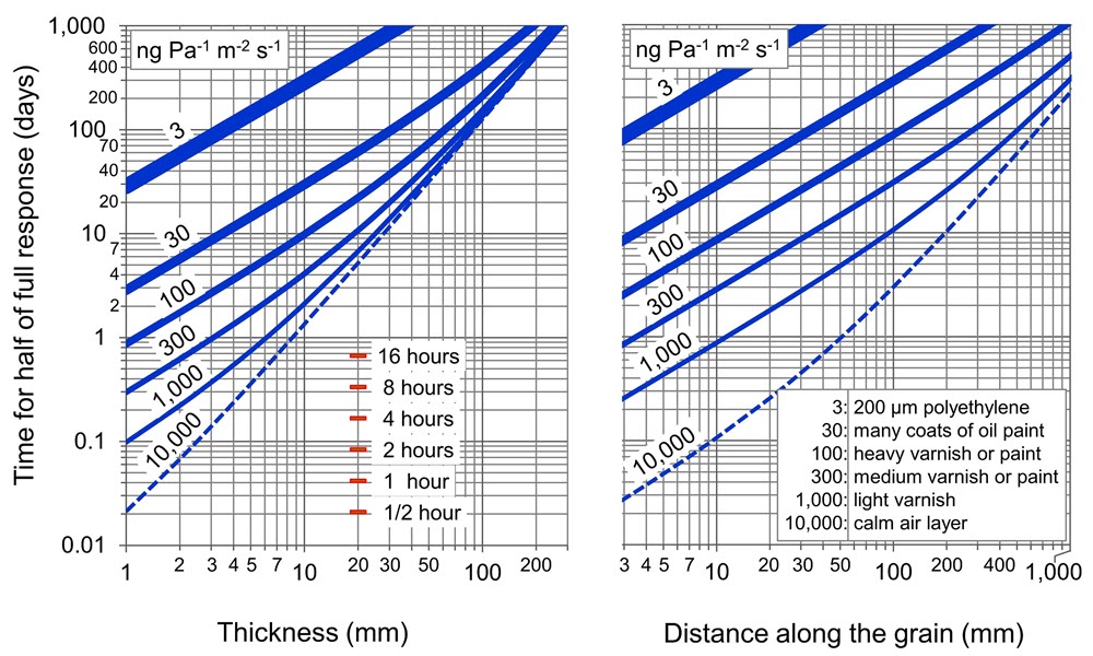
Charts for the response time of wooden objects
Wooden objects form a large part of many heritage collections. Since their thicknesses range from about a millimetre to almost a metre, and given the square law noted earlier, the response times of wooden objects vary from minutes to years. The wide variety of coatings on wood further complicates predictions. Some common objects have been listed previously in Table 4, but Figures 3 and 4 provide a more complete map of the phenomenon and also show the enormous benefits of wrapping wooden objects in airtight polyethylene film when not on display.
© Government of Canada, Canadian Conservation Institute. 132715-0034
Figure 3. Response time in days (near 20°C) of medium-density wood to RH changes. Left graph for across the grain, right graph for along the grain. This assumes both sides (or both ends) are exposed.
Description for Figure 3
Figure 3 contains two graphs, side by side. Both share a vertical axis labelled “Time for half of full response (days).” The horizontal axis of the left graph provides the thickness in millimetres. On the right graph, the axis provides the distance along the grain in millimetres. Each graph has six plots. All plots slope smoothly from bottom left to top right and appear to converge at top right. Key points along the six plots of the left-hand graph and right-hand graph are provided in Table 5 and Table 6, respectively.
| Permeance ng/Pa/m2/s |
Example of a coating with this permeance | 1 mm thick | 2 mm thick | 5 mm thick | 10 mm thick | 20 mm thick | 50 mm thick | 100 mm thick | 200 mm thick |
|---|---|---|---|---|---|---|---|---|---|
| 3 | 200 µm polyethylene | 30 | 60 | 140 | 300 | 600 | 1,500 | 3,000 | 6,000 |
| 30 | Many coats of oil paint | 3 | 6 | 15 | 30 | 60 | 170 | 400 | 1,000 |
| 100 | Heavy varnish or paint | 0.9 | 2 | 5 | 10 | 22 | 80 | 200 | 700 |
| 300 | Medium varnish or paint | 0.3 | 0.6 | 2 | 4 | 10 | 50 | 150 | 600 |
| 1,000 | Light varnish | 0.1 | 0.2 | 1 | 2 | 7 | 36 | 130 | 500 |
| 10,000 | Calm air layer | 0.02 | 0.07 | 0.4 | 1 | 5 | 32 | 130 | 500 |
* Some values are off the range of the graph.
Technical note for Tables 5 to 8: permeance is a measure of the rate of moisture transfer across a layer of material as a function of the vapour pressure of water acting across that layer.
| Permeance ng/Pa/m2/s |
Example of a coating with this permeance | 5 mm thick | 10 mm thick | 20 mm thick | 50 mm thick | 100 mm thick | 200 mm thick | 500 mm thick | 1 m thick |
|---|---|---|---|---|---|---|---|---|---|
| 3 | 200 µm polyethylene | 140 | 300 | 600 | 1,500 | 3,000 | 6,000 | 14,000 | 30,000 |
| 30 | Many coats of oil paint | 14 | 30 | 60 | 140 | 300 | 600 | 1,500 | 3,000 |
| 100 | Heavy varnish or paint | 4 | 9 | 20 | 40 | 90 | 200 | 500 | 1,000 |
| 300 | Medium varnish or paint | 1.4 | 3 | 6 | 15 | 30 | 70 | 200 | 500 |
| 1,000 | Light varnish | 0.4 | 1 | 2 | 5 | 11 | 25 | 100 | 300 |
| 10,000 | Calm air layer | 0.05 | 0.1 | 0.3 | 1 | 3 | 10 | 60 | 200 |
* Some values are off the range of the graph.
The graph on the left side of Figure 3 and its selected values in Table 5 consider a plank of wood exposed on both faces. The graph on the right side of Figure 3 and its selected values in Table 6 consider a wooden object exposed only on its end grain. For objects that have both kinds of directions exposed, first find both sets of predictions, and then select the shortest time, which will still overestimate the response time somewhat.

© Government of Canada, Canadian Conservation Institute. 132715-0036
Figure 4. Dependence of response time in days (near 20°C) of a wooden cabinet or chest of drawers as the width of the gaps at the top and bottom increases. (Object is 1.5 m high, 1 m wide, 0.5 m deep; wood thickness is 1 cm; gaps are 15 mm deep and extend from side to side.)
Description for Figure 4
Figure 4 contains two graphs, side by side. Both share a vertical axis labelled “Time for half of full response (days).” The horizontal axis of both graphs provides the gap width in millimetres. There are six plots in each graph, all similarly S-shaped. Key points along the six plots of the left-hand graph and the right-hand graph are provided in Table 7 and Table 8, respectively.
| Permeance ng/Pa/m2/s |
Example of a coating with this permeance | 0.1 mm gap | 0.5 mm gap | 0.7 mm gap | 1 mm gap | 2 mm gap | 3 mm gap | 5 mm gap |
|---|---|---|---|---|---|---|---|---|
| 3 | 200 µm polyethylene | 600 | 400 | 250 | 120 | 20 | 10 | 7 |
| 30 | Many coats of oil paint | 60 | 60 | 50 | 40 | 14 | 7 | 4 |
| 100 | Heavy varnish or paint | 20 | 20 | 20 | 20 | 10 | 6 | 3 |
| 300 | Medium varnish or paint | 11 | 11 | 11 | 10 | 7 | 4 | 2 |
| 1,000 | Light varnish | 7 | 7 | 7 | 7 | 5 | 3 | 2 |
| 10,000 | Calm air layer | 6 | 6 | 6 | 6 | 4 | 3 | 2 |
| Permeance ng/Pa/m2/s |
Example of a coating with this permeance | 0.1 mm gap | 0.5 mm gap | 0.7 mm gap | 1 mm gap | 2 mm gap | 3 mm gap | 5 mm gap |
|---|---|---|---|---|---|---|---|---|
| 3 | 200 µm polyethylene | 4,000 | 3,000 | 2,000 | 1,000 | 140 | 40 | 9 |
| 30 | Many coats of oil paint | 500 | 500 | 400 | 350 | 100 | 40 | 9 |
| 100 | Heavy varnish or paint | 200 | 200 | 170 | 150 | 80 | 35 | 9 |
| 300 | Medium varnish or paint | 90 | 90 | 90 | 80 | 55 | 30 | 8 |
| 1,000 | Light varnish | 60 | 60 | 60 | 50 | 40 | 25 | 8 |
| 10,000 | Calm air layer | 45 | 45 | 45 | 45 | 35 | 20 | 8 |
Figure 4 and Tables 7 and 8 consider wooden furniture that is coated on the outside but not the inside. Such furniture may have drawers or doors with gaps at the top and bottom, which allow exterior air to flow in and come in contact with the bare wood interior. Although such furniture in a museum is usually empty and often open for display of the interior, historically, such furniture was closed as well as filled with clothing or bedding, which would have been an excellent humidity buffer.
In Figure 4, the horizontal plateaus on the left are regions where air leakage through gaps is insignificant and the wood coating dominates half-time. The plots drop drastically on the right as the air leakage through cracks dominates. On the far right, the plots begin to bend upwards as the air leakage into the furniture interior is so large that the pieces of wood, which are uncoated on the inside, behave simply as fully exposed slabs of wood that are coated on only one side. (This final stage of behaviour, which affects only the left-hand graph, was not considered in versions of the figure that appear in the 1999, 2019 and 2023 editions of the ASHRAE Handbook.)
The lessons from Figure 4 and Tables 7 and 8 are that this type of furniture, that was usually closed, well fitted and full of textiles, could have survived large fluctuations in RH for many weeks or even months, historically. However, when the furniture was empty in a museum, it was much more responsive to short fluctuations. If left permanently open, the furniture reverts to the times of exposed wood pieces, given in Figure 3 and Tables 5 and 6. Finally, for single pieces of wood, well-sealed heavy-gauge polyethylene film offers stability well beyond one year if you avoid gaps in the packaging.
Concerns about temperature fluctuations on microclimate enclosures
An inevitable concern with enclosures is the humidity fluctuation driven by a thermal fluctuation. This worry first emerged in the 1960s for works of art in shipping crates, but Toishi (1959) showed that if a sealed crate contained hygroscopic material, it would stabilize its RH despite drops from room temperature to freezing and back. Stolow (1966) provided complete data and equations for the counterintuitive result that with natural hygroscopic materials, the humidity in the enclosure even drops slightly when the temperature drops (the opposite of empty enclosures) due to the slight shift downwards of moisture isotherms at lower temperatures.
Thomson (1964) showed that the transition point between RH-controlled enclosures (RH is stable or drops slightly) and mostly uncontrolled empty enclosures for hygroscopic materials such as wood occurred when there was about 1 kg of material per cubic metre of enclosure. Humidity control was fully in place when 10 kg of material was present in each cubic metre of enclosure (about 2% by volume). Later authors have examined further side effects such as mixed thermal/hygric dimensional response in wood (Richard 2007) and condensation in air pockets during cold-storage retrieval (Padfield 2002; Shashoua 2005, 2008), but the consensus is that such occasional side effects do not outweigh the benefits (Richard 2007; Shashoua 2014).
The effect of temperature on response times
Lower temperatures greatly increase response times and, conversely, higher temperatures shorten them. This has been demonstrated in measurements of archival materials (Adelstein et al. 1997). You can estimate that response times, such as those in Tables 5, 6, 7 and 8 and in Figure 3, which are for 20°C, will double for each drop of 10°C (for example, ×2 for storage at 10°C, ×4 for storage at 0°C, ×8 or more for storage at -10°C). The cause is the drop in the diffusion coefficient of moisture in solids as the temperature drops. The estimates for the chest of drawers, Figure 4 and Tables 7 and 8, will also see the times double with each decrease of 10°C, but for slightly different reasons. When the gaps are too small to affect half-times (the left-hand plateaus in the graph), the reasons are the same as above. When gap leakage dominates half-times, the reason is that the moisture capacity of infiltrating air drops by half for each 10°C drop.
Equations behind the calculations of response time
The response time of a plate (a shape that applies to many cultural objects and that provides an upper bound to cylinders, cubes, spheres, etc.) is given by Crank (1979) as the following:
Equation 2: t½ = 0.049 * d2 / D
Where
t1/2 = half-time of the microclimate enclosure, seconds
d = thickness of plate (or sheet), m
D = diffusion coefficient m2/s
Values of the diffusion coefficient can be found in various handbooks, such as Siau (2012) for wood, and Park and Crank (1968) for polymers.
The humidity half-time of a leaky enclosure with a hygroscopic material (objects or additional buffers) can be expressed in terms of the fraction of the enclosure volume filled with the buffering material (Michalski 1994, eqn. 39):
Equation 3: t½ = 0.69 * (Vh * α * ρ) / (N * Ve * Cws)
Where
t1/2 = half-time of the microclimate enclosure, seconds, hours or days (depends on leakage units)
Vh = volume of the hygroscopic material, m3
Ve = volume of the enclosure, m3
α = hygric capacity (slope of the moisture isotherm) kg/kg
ρ = bulk density of the hygroscopic material, kg/m3
N = leakage, expressed as air changes per second, per hour or per day
Cws = concentration of water in the air at saturation, kg/m3
The critical role of leakage (N) for enclosed objects can be seen by following the example in Table 4 of paintings or works of art on paper in a sealed glass frame (increasingly used by major galleries, especially for loaned paintings). Depending on tiny differences in crack width, performance can change by several orders of magnitude. This is due to the key role of infiltration in determining N and the fact that infiltration through narrow cracks varies with the cube of crack width; that is, reducing crack width by a factor of 2 will reduce air infiltration by a factor of 8 (Michalski 1994).
Equation 1 can be reduced to an estimate for materials such as paper, wood, leather and dense fabrics near room temperature, 20°C, where Cws = 0.0173 kg/m3. Using a conservative density where ρ is about 600 kg/m3 and a conservative hygric capacity where α is about 0.05, then
Equation 4: t½ = 1200 * Vh / (N * Ve)
A leakage rate of 1 air change per day (ACD) is considered a suitable design target for airtight museum display cases (Thickett et al. 2007), so an enclosure half full of wood or paper (Vh/Ve = 1/2) would give a half-time of 600 days. In practical terms, very tight enclosures are rarely very full enclosures (although wrapping large wooden objects in heavy-gauge, perfectly sealed polyethylene can achieve this). Half-full enclosures are generally cabinets or crates, and they leak closer to 1 air change per hour (ACH), which still provides a 25-day half-time. A tight display case of 1 ACD will rarely have more than 10% of its volume filled with hygroscopic material, resulting in half-times up to 120 days. In practice, it is difficult but not impossible to design and maintain very low infiltration (Thickett et al. 2007).
Some estimates in Table 4 are based on this equation and diffusion coefficients found in the literature on polymers. An object with a surrounding moisture barrier (coating or enclosure) can be simplified as a series of two resistances to moisture flow. Figure 3 was generated using this approach with wood data from Siau (2012) for medium-density wood near 50% RH. When barriers provide useful resistance (consult the upper lines in each plot in Figure 3), the plots have a slope of 1 (linear). When coatings provide negligible resistance, such as the boundary layer of air in a calm room, the slope of the plots changes to the square law of equation 1. There is only a slight curve as thickness drops to 1 mm across the grain. Kupczak (2018) has measured the contribution of the boundary layer of air, which is measurable but far from being rate determining, even for a single sheet of paper. In practical terms, thinner objects respond more quickly (for example, a violin, ivory miniature and paper sheet), but they also benefit much more than thicker objects from even simple coatings or enclosures (such as cases, cabinets and packaging).
Figure 4 was generated by using the same series resistance model but by using leakage equations for an enclosure found in Michalski (1994). Besides the assumption of the dimensions noted in the caption for Figure 4, the graph also assumes that the typical stack pressure driving air infiltration is due to either a 1°C temperature difference or a 40% RH difference. Consult Michalski (1994) for further explanation of these numbers.
Bibliography
Adelstein, P.Z., J.-L. Bigourdan and J.M. Reilly. “Moisture Relationships of Photographic Film.” Journal of the American Institute for Conservation 36,3 (1997), pp. 193–206.
American Society of Heating, Refrigerating and Air-Conditioning Engineers. “Museums, Libraries and Archives.” In R. Parsons, ed., ASHRAE Handbook: Heating, Ventilating and Air-Conditioning Applications, Atlanta, GA: ASHRAE, 1999, pp. 20.1–20.13.
American Society of Heating, Refrigerating and Air-Conditioning Engineers. “Museums, Galleries, Archives, and Libraries.” In M.S. Owen, ed., ASHRAE Handbook: Heating, Ventilating, and Air-Conditioning Applications. Atlanta, GA: ASHRAE, 2019, pp. 24.1–24.46.
American Society of Heating, Refrigerating and Air-Conditioning Engineers. “Museums, Galleries, Archives, and Libraries.” In M.S. Owen, ed., ASHRAE Handbook: Heating, Ventilating, and Air-Conditioning Applications. Atlanta, GA: ASHRAE, 2023, pp. 24.1–24.47.
Batterham, I., and J. Wignell. “The Mitigating Effects of Packaging on Temperature and Humidity Fluctuations.” In P. McKay and A. Treasure, eds., 5th AICCM Book, Paper and Photographic Materials Symposium, 2008, pp. 11–16.
Bigourdan, J. “Understanding Temperature and Moisture Equilibration: A Path Towards Sustainable Strategies for Museum, Library and Archives Collections.” Presentation at the 10th Annual Indoor Air Quality Conference. London, UK, June 17–20, 2012.
Bratasz, Ł., and M.R. Vaziri Sereshk. “Crack Saturation as a Mechanism of Acclimatization of Panel Paintings to Unstable Environments.” Studies in Conservation 63, Suppl. 1 (2018), pp. 22–27.
Crank, J. The Mathematics of Diffusion. Oxford, UK: Oxford University Press, 1979.
Derluyn, H., H. Janssen, J. Diepens, D. Derome and J. Carmeliet. “Hygroscopic Behavior of Paper and Books.” Journal of Building Physics 31,1 (July 2007), pp. 9–34.
Di Pietro, G., and F.J. Ligterink. “Prediction of the Relative Humidity Response of Backboard-Protected Canvas Paintings.” Studies in Conservation 44,4 (January 1999), pp. 269–277.
Ekelund, S., P. Van Duin, A. Jorissen, B. Ankersmit, and R.M. Groves. “A Method for Studying Climate-related Changes in the Condition of Decorated Wooden Panels.” Studies in Conservation 63,2 (2018), pp. 62–71.
Hackney, S. “Framing for Conservation at the Tate Gallery.” The Conservator 14,1 (1990), pp. 44–52.
Hagan, E. “Acoustic Emission Analysis of Humidity-induced Damage to Model Wood Structures.” Lecture presented at the “Mechanics for Art Conservation” [online workshop]. International Institute for Conservation of Historic and Artistic Works, December 2021.
Karsten, I., S. Michalski, M. Case and J. Ward. “Balancing the Preservation Needs of Historic House Museums and Their Collections Through Risk Management.” In K. Seymour and M. Sawicki eds., Proceedings of the Joint Conference of ICOM-DEMHIST and Three ICOM-CC Working Groups: The Artifact, Its Context and Their Narrative: Multidisciplinary Conservation in Historic House Museums, Los Angeles, CA, 6–9 November, 2012. N.p.: International Council of Museums – Committee for Conservation and Committee for Historic House Museums, 2012.
Kupczak, A., Ł. Bratasz, J. Kryściak-Czerwenka and R. Kozłowski. “Moisture Sorption and Diffusion in Historical Cellulose-based Materials.” Cellulose 25 (April 2018), pp. 2873–2884.
Lafontaine, R.H., and P.A. Wood. “The Stabilization of Ivory against Relative Humidity Fluctuations.” Studies in Conservation 27,3 (August 1982), pp. 109–117.
Michalski, S. “Relative Humidity: A Discussion of Correct/Incorrect Values.” In J. Bridgland, ed., ICOM Committee for Conservation 10th Triennial Meeting, Washington, D.C., 22–27 August 1993: Preprints, vol. 2. London, UK: James & James Ltd./ICOM-CC, 1993, pp. 624–629.
Michalski, S. “Leakage Prediction for Buildings, Cases, Bags and Bottles.” Studies in Conservation 39,3 (August 1994), pp. 169–186.
Michalski, S. “Climate Control Priorities and Solutions for Collections in Historic Buildings.” Historic Preservation Forum 12,4 (1998), pp. 8–14.
Michalski, S. “Risk Analysis of Backing Boards for Paintings: Damp Climates vs Cold Climates.” In CESMAR7, ed., Minimo intervento conservativo nel restauro dei dipinti: Atti del convegno, Thiene (VI), 29–30 ottobre 2004, Secondo congresso internazionale, Colore e conservazione materiali e metodi nel restauro delle opere policrome mobili. Saonara, Italy: Il Prato, 2005, pp. 21–27.
Michalski, S. “The Ideal Climate, Risk Management, the ASHRAE Chapter, Proofed Fluctuations, and Toward a Full Risk Analysis Model” (PDF Format). In F. Boersma, ed., Contribution to the Experts’ Roundtable on Sustainable Climate Management Strategies, April 2007, Tenerife, Spain. Los Angeles, CA: J. Paul Getty Trust, 2007.
Michalski, S. “The Power of History in the Analysis of Collection Risks from Climate Fluctuations and Light.” In J. Bridgland, ed. ICOM Committee for Conservation 17th Triennial Meeting, Melbourne, 15–19 September 2014, Preprints. Paris, France: ICOM-CC, 2014, pp. 1–8.
Michalski, S. “Climate Guidelines for Heritage Collections: Where We Are in 2014 and How We Got Here.” In S. Stauderman and W.G. Tompkins, eds., Proceedings of the Smithsonian Summit on the Museum Preservation Environment (PDF format). Washington, D.C.: Smithsonian Institution Scholarly Press, 2016, pp. 7–32.
Padfield, T. “Condensation in Film Containers During Cooling and Warming” (PDF format). In D. Niseen et al., eds., Preserve Then Show. Copenhagen, Denmark: The Danish Film Institute, 2002.
Park, G.S., and J. Crank, eds. Diffusion in Polymers. New York, NY: Academic Press, 1968.
Richard, M. “The Benefits and Disadvantages of Adding Silica Gel to Microclimate Packages for Panel Paintings.” In T. Padfield et al., eds., Museum Microclimates: Contributions to the Copenhagen Conference 19–23 November 2007. Copenhagen, Denmark: National Museum of Denmark, 2007, pp. 237–243.
Shashoua, Y. “Storing Plastics in the Cold: More Harm than Good?” In J. Bridgland, ed., ICOM-CC 14th Triennial Meeting, The Hague, The Netherlands, 12–16 September 2005: Preprints, vol. 1. London, UK: James & James/Earthscan, 2005, pp. 358–364.
Shashoua, Y. Conservation of Plastics: Materials Science, Degradation and Preservation. Oxford, UK: Butterworth-Heinemann (Elsevier), 2008.
Shashoua, Y. “A Safe Place: Storage Strategies for Plastics.” Conservation Perspectives (Spring 2014), pp. 13–15.
Siau, J.F. Transport Processes in Wood. Berlin, Germany: Springer Science & Business Media, 2012.
Stillwell, S.T.O., and R.A.G. Knight. “Appendix I. An Investigation into the Effect of Humidity Variations on Old Panel Paintings on Wood.” In Some Notes on Atmospheric Humidity in Relation to Works of Art. London, UK: Camelot Press Limited, 1934, pp. 17–34.
Stolow, N. Controlled Environment for Works of Art in Transit. London, UK: Butterworths, 1996.
Thickett, D., P. Fletcher, A. Calver and S. Lambarth. “The Effect of Air Tightness on RH Buffering and Control.” In T. Padfield et al., eds., Museum Microclimates: Contributions to the Copenhagen Conference 19–23 November 2007. Copenhagen, Denmark: National Museum of Denmark, 2007, pp. 245–251.
Thomson, G. “Relative Humidity: Variation with Temperature in a Case Containing Wood.” Studies in Conservation 9,4 (November 1964), pp. 153–169.
Toishi, K. “Humidity Control in a Closed Package.” Studies in Conservation 4,3 (August 1959), pp. 81–87.
Wu, X.-F., R.A. Jenson and Y. Zhao. “Stress-Function Variational Approach to the Interfacial Stresses and Progressive Cracking in Surface Coatings.” Mechanics of Materials 69,1 (2014), pp. 195–203.
© Government of Canada, Canadian Conservation Institute, 2025
Published by:
Canadian Conservation Institute
Department of Canadian Heritage
1030 Innes Road
Ottawa ON K1B 4S7
Canada
Cat. No.: CH57-4/83-2025E-PDF
ISBN 978-0-660-75636-3